Using camera traps to compare the habitat choice of different deer species in hunting versus non-hunting season

(1)

Department of Wildlife, Fish, and Environmental Studies

Using camera traps to compare the habitat

choice of different deer species in hunting

versus non-hunting season

(2)

(3)

Using camera traps to compare the habitat choice of different

deer species in hunting versus non-hunting season

Laura Juvany Canovas

Supervisor: Tim Hofmeester, Swedish University of Agricultural Sciences, Department of Wildlife, Fish, and Environmental Studies

Assistant supervisor: Joris Cromsigt, Swedish University of Agricultural Sciences, Department of Wildlife, Fish, and Environmental Studies

Assistant supervisor: Patrick Jansen, Wageningen University & Research, Department of Environmental Sciences

Examiner: Fredrik Widemo, Swedish University of Agricultural Sciences, Department of Wildlife, Fish, and Environmental Studies

Credits: 30 credits

Level: Second cycle, A2E

Course title: Master degree thesis in Biology at the department of Wildlife, Fish, and Environmental Studies

Course code: EX0633

Course coordinating department: Department of Wildlife, Fish, and Environmental Studies

Place of publication: Umeå

Year of publication: 2019

Cover picture: From camera traps

Title of series: Examensarbete/Master's thesis

Part number: 2019:3

Online publication: https://stud.epsilon.slu.se

Keywords: ungulates, camera trapping, occupancy modelling

(4)

(5)

Abstract

A general increase in ungulate populations calls for a better understanding of their habitat use and movement at small spatial scales. This understanding is necessary for the development of useful management actions to solve possible human-wildlife conflicts. One proposed management action is to use the indirect effects of hunting. Hunting activities potentially increase the feeling of risk of being predated perceived by ungulates, which could decrease their fitness by choosing to move to less risky areas with a lower quality of food. In this study, I wanted to determine how habitat use of ungulates changed between seasons in a peninsula in northern Sweden where four species of ungulates coexist: moose (Alces alces), roe deer (Capreolus

capreolus) red deer (Cervus elaphus) and fallow deer (Dama dama). I hypothesized

that during the hunting period ungulate habitat selection would be driven by hunting risk perception, which would imply a stronger selection for forest sites with low visibility (high denseness of understory vegetation), than for forest sites with high visibility. Outside of the hunting period, I hypothesized that habitat selection would be driven by food availability and preference, making ungulates choose the most productive areas. To study this, I used data collected with camera traps, from which I obtained the passages for the four ungulate species and built models for naïve occupancy, occupancy and passage rates to determine which habitat type was more visited per season and species. I found different habitat selection patterns for three of the four studied species. Most notably, passage rates of moose were higher in open sites outside of the hunting season, while there was no difference between the habitat types during the hunting period. These differences give an insight in the importance of developing specific management per species even if they are situated in a multispecies system. My research confirms that hunting could potentially be used as a management strategy to change the habitat selection of moose away from open areas, such as planted clear-cuts.

(6)

Data analysis ... 13 Naïve occupancy ... 13 Occupancy models ... 13 Passage rates ... 15 Results ... 16 Naïve occupancy ... 16 Occupancy models ... 20 Passage rates ... 22 Discussion ... 26 Acknowledgements ... 30 Literature cited ... 31 Appendix ... 34 Appendix 1 ... 34 Appendix 2 ... 35 Appendix 3 ... 36

(7)

Introduction

Populations of ungulates are showing a global tendency to increase, particularly in Europe (Apollonio, Andersen & Putman 2010; Cromsigt et al. 2013), where large populations of these species can lead to human-wildlife conflicts (Cromsigt et al. 2013) such as damage to agriculture and forestry (Kuijper 2011). There is evidence that ungulate spatial distribution is dependent on food quality, as they select areas from which the highest input of protein and energy can be obtained (Wilmshurst & Fryxell 1995; Kuijper et al. 2009). When taking into account forested areas, clear cut systems have been found to be more preferred as foraging systems than closed forest patches. Clear cut areas have a higher light level which lead to increased regeneration and vegetation growth, but this also causes an increase in the C:N ratio, decreasing food quality of plants (Kuijper et al. 2009). This could mean that ungulates with a feeding strategy to select for high quality resources will select young trees in closed forest, and those selecting for food quantity will make use of clear cuts.

Habitat selection does not only depend on food availability and quality, but also on the hunting risk perceived by a prey (Cromsigt et al. 2013). Ungulates feeding in open areas perceived a higher risk, showing an increased vigilance time, than the ones in closed forested areas (Benhaiem et al. 2008; Bonnot et al. 2013). This behaviour is linked to the fact that woodlands provide a better shelter to escape from some predators and hunters (Benhaiem et al. 2008). Hunting activity is higher in open areas due to an increased visibility from hunters, which has been found to affect habitat preference towards closed and dense forested areas in large herbivores (McLoughlin et al. 2011).

There is an increased evidence that human disturbances such as hunting can lead to direct and indirect modifications on ungulate and other wildlife populations (Neumann, Ericsson & Dettki 2009). Cromsigt et al. (2013) examined the possibility of introducing ‘hunting for fear’ as a tool to manage increasing ungulate populations. This is based on the ‘ecology of fear’ hypothesis (Brown, Laundré & Gurung 1999) which postulates that prey populations are not only influenced by the number of animals a predator kills, but also by indirect effects; i.e., the fear of being predated causes prey to change its behaviour and move from preferred sites to less risky areas. Ungulate habitat use is determined by the trade-off between foraging needs and predation avoidance (Proffitt 2009) and resource quality is often positively correlated with areas with a higher human-related source of risk (Bonnot et al. 2013). There is evidence that hunting risk indeed changes habitat use of ungulates on large temporal scales (Bonnot et al. 2013; Benhaiem et al. 2008; McLoughlin et al. 2011), avoiding open areas with a higher hunting risk during day in the hunting season. Vegetation cover has

(8)

been found to also play an important role in predator avoidance. When avoiding human predation, habitat with a high vegetation cover offers a safer environment for ungulates, as they become less visible to hunters (Lone et al. 2014). However, we know very little about the behavioural responses to hunting on smaller spatial scales, which should not only fit socio-political entities (as municipality or province) but completely fit the species occurrence, which are needed for a ‘hunting for fear’ management strategy (Cromsigt et al. 2013). Also, as ungulate assemblages are becoming more diverse, studies are needed on how different species react in a multi-species system (Vabra & Riggs, 2010).

Different hunting practices lead to differences in ungulate behaviour (Cromsigt et al. 2013). It has been found that when compared to other hunting practices, hunting with dogs increase the risk perception and stress levels of ungulates (Ericsson, Neumann & Dettki, 2009). Even though this practise has been banned in some countries of the European Union, in Scandinavia is common and largely practised. Ungulates can also be affected during the training of dogs and when hunting aims other species. Present hunting practices are highly predictable temporal and spatially, which can sometimes be a disadvantage as ungulates can avoid it to some extent (Cromsigt et al. 2013).

In this study I aim to analyse the visitation of different forest sites by moose (Alces alces), roe deer (Capreolus capreolus), red deer (Cervus elaphus) and fallow deer (Dama dama) during hunting and non-hunting seasons in the Järnäshalvon peninsula, Sweden. The coexistence of these four ungulate species is quite rare in Sweden, which makes this peninsula a good case of study to improve the knowledge on how to manage multi-species systems. Forest sites were classified in four groups, depending if they were open or closed forest with low or highly dense understorey, which determines how the habitat gives high or low visibility respectively. Five different seasons were tested separately: non-hunting season, hunting season, training of hunting dogs, rutting during hunting period (only for red deer) and break during the hunting season period (only for moose). To investigate this, I used movement pictures from camera traps, analysing the passages of the four ungulate species by building models for their naïve occupancy, occupancy and passage rates to determine which of the four types of habitat was visited to a greater extent along the different seasons.

Differences expected among the studied species can be driven by three main aspects: habitat preference due to food availability, hunting method applied to each species and the fact that each species differ in extension of hunting periods.

(9)

Moose is the largest of the four ungulate species and is included in the feeding type of concentrate selectors (Hofmann 1989). This species digestive system is less efficient in optimizing plant fibre digestion, so they need higher quality food, with low ratios of C:N. Roe deer is also described as a concentrate selector, feeding only on the high quality parts of plants, but when compared to moose body size, this species will need a smaller amount of daily intake vegetation (Hofmann 1989). As both species are selectors, they are able to feed on the most nutritious vegetation parts in every habitat type. Red deer is classified as an intermediate feeder, as it feeds on pasture and grasses during the periods of juvenile growth, lactation and when they need to create reserves before winter and rutting period (Hofmann 1989). This type of vegetation suits these purposes, occurring with higher abundance but with lower quality (Kuijper et al. 2009). In autumn, this species become browsers and decrease their metabolism as they are not as efficient as concentrate selectors in digesting high fibre content food (Hofmann 1989). Lastly, fallow deer is the ungulate species with the closest diet composition to grazers, and is classified in between intermediate feeders and grass eaters, meaning that their diet composition is mainly driven by the quantity of vegetation available (Hofmann 1989).

In this study I will test how the habitat variables of openness and visibility play a role in risk perception from human hunting by ungulates. I classified each of the studied sites into open or closed forest canopy, with high or low visibility due to denseness of vegetation cover. I hypothesize that during the no hunting season, ungulates habitat preference will be driven by food availability, selecting the most productive areas in terms of food quantity, where even selective feeders are able to choose the most nutritious vegetation (Hofmann 1989, Bouyer et al. 2015). I expect these species to select open habitats with low visibility due to dense understorey vegetation the most, followed by closed forest with low visibility and open with high visibility, and lastly closed forest with high visibility.

I hypothesize that hunting risk is a major driver in habitat selection, and ungulates will have to trade-off between selecting habitats that give them a lower risk perception, and those habitats with a better food availability. There is evidence of ungulates selecting lower risk areas under human hunting pressure periods (Bonnot et al. 2013; Benhaiem et al. 2008; McLoughlin et al. 2011; Lone et al. 2014). In Gehr et al. (2017) they even found that roe deer reacted strongly to human hunting than to other predators as lynx (Lynx lynx), avoiding open habitats during day time in the hunting season. During the hunting period I expect that visibility will play a more important role than the openness of the canopy, so I hypothesize that ungulates will select closed and open forests with low visibility to a major extent, followed by open and closed forest sites with a high visibility.

(10)

Dogs that are training or that are being used by hunters but aiming at other species will also disturb ungulates but to a lower extent when compared to the hunting period. I hypothesize that this disturbance will also make the ungulates to choose the sites with lower visibility, so I do not expect to find differences in habitat selection between this period and the hunting period. In this study I also considered the rutting period jointly with hunting for red deer. Rutting has been seen to increase the activity of ungulates (Neumann & Ericsson 2018). I hypothesize that this species will select open or closed forest habitats but with low visibility. Hunting will be the driver to select for less risky habitats, and rutting will increase their activity when compared to other periods. I will also include the break during the hunting period for moose, during which dogs that aim for other species will still be in the area. Taking this into account I expect the same results for this period as during the dog training period.

(11)

Materials and methods

Area of study and experimental design

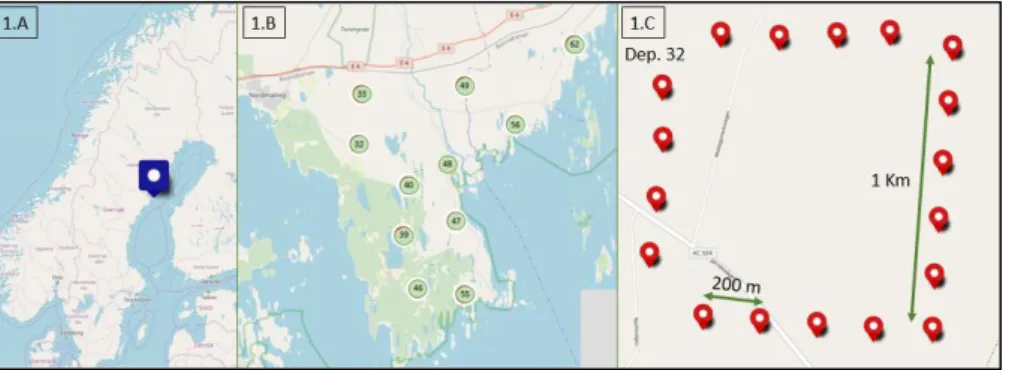
The study area is situated in the Järnäshalvön peninsula located in the Västerbotten county in northern Sweden (see figure 1.A). This 200 km2

peninsula is surrounded by the Baltic Sea on its southern part, and by a fenced highway and railway on its northern part, making it a relatively isolated area. Nordmaling and Hörnefors are the main towns in the area, bordering the peninsula in the north-west and north-east sides. Inside the peninsula there are also a few smaller urban areas.

For this study I used data from an ongoing research for which eleven tracts as hollow grids of 1x1 km were randomly placed in non-urbanized areas of the peninsula with an average of 1.8 km distance between tracts (see figure 1.B). Each hollow grid contained 3 cameras (Reconyx Hyperfire HC 500) at any time with a separation of 200 m between camera locations (see figure 1.C). Cameras were rotated within the hollow grids every 6-8 weeks forming rounds (six per year), and resulting in 18 deployments of 6-8 weeks per tract. Cameras were placed on trees 50cm-1m above ground and facing in a direction with at least 15 meters open visibility.

Figure 1: 1.A shows the location of the study area, the Järnashälvön peninsula in the county of Västerbotten in north Sweden. In 1.B we can observe the eleven tracts placed inside the peninsula, and in 1.C the hollow grid of 1x1 km, with 18 camera sites per tract.

Species of study

Moose (Alces alces), roe deer (Capreolus capreolus), red deer (Cervus elaphus) and fallow deer (Dama dama) occur in this area and will be the focus of this study.

Moose has changed from relatively rare to a dominant species in Sweden during the last 100 years (Lavsund, Nygén & Solberg 2003). Red deer and

(12)

roe deer arrived in Sweden after the last ice age via the land bridge that connects Denmark and Sweden. Red deer have been increasing their range towards northern Sweden (Apollonio, Andersen & Putman 2010), and were introduced in the study area in the 1970s when they escaped from enclosures introduced by T. Gadelius (Pfeffer 2016). Fallow deer is considered an exotic species introduced in Sweden as early as the seventeenth century (Apollonio, Andersen & Putman 2010). Jointly with the red deer, 12 to 15 individuals of fallow deer escaped from the enclosure from T. Gadelius in the Järnäshalvön peninsula (Pfeffer 2016), and this is the most northern site where they can be seen in Sweden.

Study period and hunting periods

In this study we selected a subset of the one year data, and analysed the pictures taken from the 1st_{of July till the 31}st_{of October. These four months}

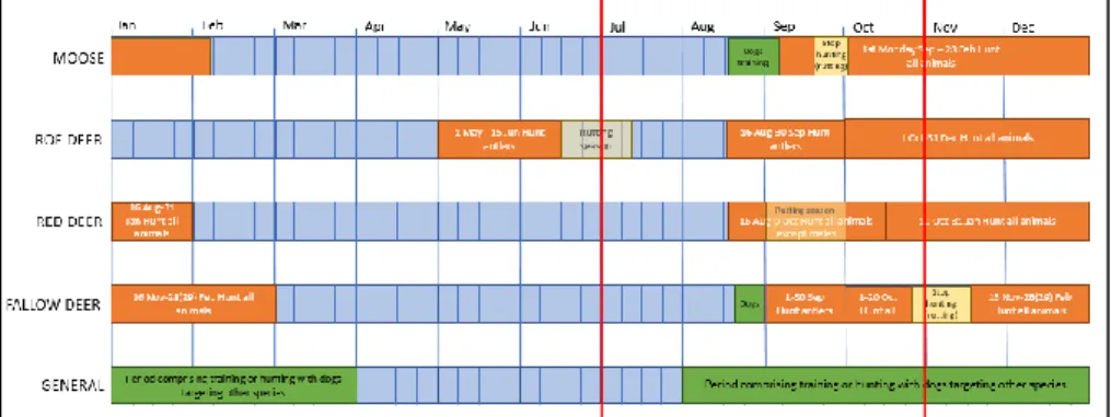
of data were selected as they coincide with important periods along the year of the four ungulates (see figure 2). We compared habitat use among four different periods; the non-hunting season, the hunting season, the season of training of hunting dogs even if they do not target these species and the rutting season. The exact timing of these periods differed among species (see figure 2 and appendix 1 for the exact dates).

Figure 2: Time line of the year events per each study species and a general one that shows events that could affect all of them. In orange we can observe the hunting periods, in which the dates and the target (all animals or only males with antlers) are indicated. In green the periods of training of hunting dogs per species are visualized, and in the general timeline the training or hunting with dogs that are targeting other species than the ungulates included in this study. In light yellow I indicate the periods of hunting break for moose and fallow deer due to rutting, and with the same colour but more transparent, the rutting season without hunting break for roe and red deer is indicated. It is important to emphasize that not only the hunting and training of dogs aimed at each species will be the events affecting them, but also the ones targeting other species. Even though I prioritized the ones targeting a species in particular as the main driver of disturbance when this overlapped with another event. The time period analysed in this study is comprised between the two red lines, from the 1st_{of July until}

(13)

I used a four months subset, which allowed me to have a more equal time periods for each treatment compared to considering the whole year of data. This period also coincides with the months in which more sequences of these four ungulates were recorded (see appendix 2).

The hunting breaks due to the rutting season for moose and fallow deer were not long enough to be considered in my analysis separately. In the case of the moose the data from the 26th_{of September until the 8}th_{of October was}

excluded from the analysis as it could lead to misinterpretations due to the influence of the rutting behaviour. For fallow deer this break from the 21st

until the 31st_{of October was included in the analyses as no hunting period.}

Only the ten first days of the hunting break coincide with the study period as these days can be considered as not majorly affected by the rutting. For fallow deer the first effects of this season start right at the end of October, leading to a peak point during November (Kindbladh 2015), so I assume that rutting did not majorly affect during this time period included in the study.

For roe deer the no-hunting period coincides with its rutting season, so these two seasons were considered together when interpreting the results for this species. I do not expect that rutting will change the habitat preference of this species during the no hunting season, but an increase in overall activity, which is not the focus of this study. Rutting season for roe deer can also extend later than the start of its hunting season.

To have a better assessment of the hunting pressure in this area for each of the species, I retrieved in June 2018 the annual hunting bags as kg per 1000Ha from Viltdata service for Nordmalding area, which can be seen in appendix 3.

Habitat classification: open versus closed forest and

low versus high visibility

Järnäshalvön is characterized mainly by boreal forest, clear cuts of different stages and edges of the forest in a lower extent. To determine the contribution of a habitat to the risk perception of the four ungulates I decided to take into account the canopy openness and the denseness of understorey as a proxy for visibility. I divided all sites in which cameras were operable during the study period based on these two characteristics. I could not include agricultural fields as open areas in this study, as there are no cameras installed in the few of this areas in the peninsula.

For the openness variable I divided each site between open and closed forest. A site was determined as closed if when analysing the pictures taken with the camera traps on the first day of set up, the canopy would cover around an 80% of the above horizon coverage of the picture. If the camera did not give

(14)

a reliable view of the canopy, a quick analysis of the understorey was done to determine if in overall, the plant species seen would be more characteristic of high or low light availability.

Regarding the visibility variable I classified the sites as giving low or high visibility. To determine the denseness of the understorey and how visible a predator would be in each site, I analysed the pictures used to determine the effective detection distance for each camera. In each site, poles were placed at consecutive 5m distance from the camera. I determined a site as low visibility if the poles from 15m distance were difficultly spotted, and as high visibility in the contrary case.

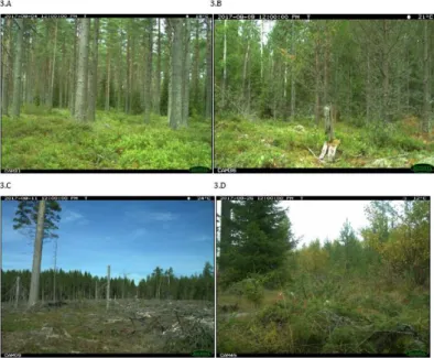
By mixing these two habitat characteristics together, I determined four different habitat types. Closed forest with high visibility sites are mainly those with older forest and almost full canopy cover, which gives low light availability for understory growth (see figure 3.A). Closed forest with low visibility are those sites with less dense canopy that allows dense understorey to grow (see figure 3.B). Open forest with high visibility are mainly recent clear cut areas with only few adult trees (normally parental trees for regeneration purposes) at the first stage of growing vegetation (see figure 3.C). Lastly, those sites that are classified as open with low visibility, which are mostly old clear cuts in which plant growth is dense and regeneration of deciduous trees advanced, which makes difficult to see further than 10m from where the camera stands (see figure 3.D).

Figure 3: Examples of the four types of habitat classification taken into account in the analysis. Image 3.A represents closed forest with high visibility, 3.B closed forest with low visibility, 3.C open forest with high visibility and 3.D open forest with low visibility. These pictures were taken on the first day each camera was set up.

(15)

Camera traps

Camera trap images were used to estimate the number of passages of the four ungulate species in this area. When a camera was triggered it would take a rapid burst of 10 consecutive pictures with no delay before the camera can be triggered again.

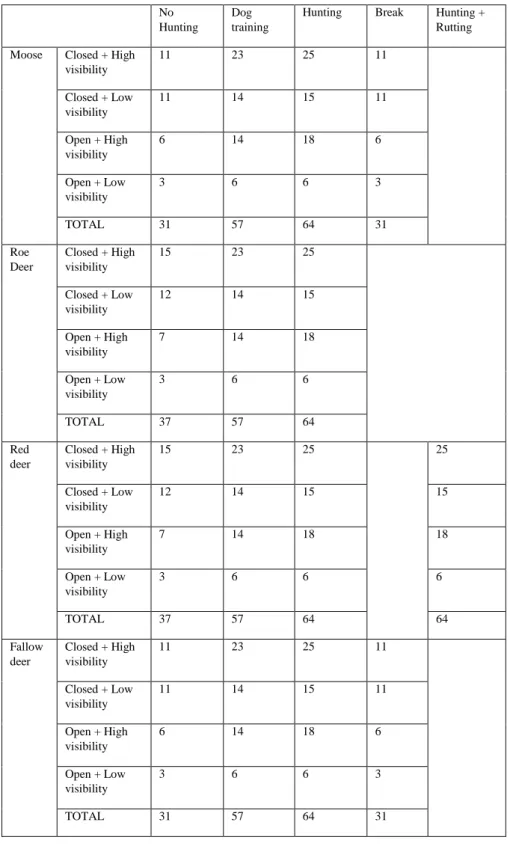
The camera trap distribution for this study aimed to include all the different habitats to have a general overview of the whole area, as it is not possible to obtain data from the complete peninsula. The number of cameras operable per season and habitat type differed per species. In overall, there were less cameras located in open areas (see table 1).

(16)

Table 1. Number of camera traps operable per species, habitat type and period considered.

No Hunting

Dog training

Hunting Break Hunting + Rutting Moose Closed + High

visibility 11 23 25 11 Closed + Low visibility 11 14 15 11 Open + High visibility 6 14 18 6 Open + Low visibility 3 6 6 3 TOTAL 31 57 64 31 Roe Deer Closed + High visibility 15 23 25 Closed + Low visibility 12 14 15 Open + High visibility 7 14 18 Open + Low visibility 3 6 6 TOTAL 37 57 64 Red deer Closed + High visibility 15 23 25 25 Closed + Low visibility 12 14 15 15 Open + High visibility 7 14 18 18 Open + Low visibility 3 6 6 6 TOTAL 37 57 64 64 Fallow deer Closed + High visibility 11 23 25 11 Closed + Low visibility 11 14 15 11 Open + High visibility 6 14 18 6 Open + Low visibility 3 6 6 3 TOTAL 31 57 64 31

(17)

Camera traps with passive infrared sensors are triggered when the difference in heat and movement between a warm animal and its colder environment exceeds a threshold (Hofmeester, Rowcliffe & Jansen 2017). This can lead to some detection issues and it is important to state that in colder regions (as the one in which this study is conducted) there is a larger difference in temperature between the animal and its environment, and when studying animals with a large body size, the detection probability of the cameras is higher (Rowcliffe et al. 2011). Camera traps have an effective detection distance (EDD), which means that the sensors cannot detect animals at an unlimited distance (Hofmeester, Rowcliffe & Jansen 2017).

It is highly important to account for several detection issues that could lead to biases when working with camera trap images to estimate ecological patterns in wildlife populations. Camera trap detection depends on three probabilities. First, the probability of an animal passing in front of the camera trap, second, the probability that this animal will trigger the camera trap, and third, the probability that this animal passes in front of the camera trap triggering it but without being able to identify it.

Data processing

Movement pictures classification and data set

I used TRAPPER (Bubnicki et al, 2016) to classify the movement pictures obtained. All pictures taken within 5 minutes were aggregated into sequences or trapping events. This procedure ensured the quantification of independent individual visits. Each sequence was classified as “Set up/Pick up” if the pictures showed the moment in which the cameras were installed or retrieved from the field, “Animal” if an animal was recorded by the camera, “Human” if a person was recorded, and “Empty” if the pictures did not show any of the previous. In very few occasions there were blank pictures due to an error when the camera took that picture or when this picture was stored in the program, these were classified as “Corrupted file”. When an animal triggered the camera and the sequence was classified as “Animal” I annotated the number of individuals, its species, sex, and age (between juvenile, sub-adult and adult).

From the picture classification I obtained a data set from TRAPPER with information per each animal recorded picture. To better analyse this data, pictures from the same sequence were aggregated per number of passages of individuals, as sometimes one sequence would include passages of more than one individual. I also included the set up and pick up date of every deployment.

(18)

Data analysis

In this study I used three different methods to determine the habitat selection of the four ungulate species during the different hunting periods: naïve occupancy, occupancy models and passage rates analysis.

Naïve occupancy

First of all, I calculated the naïve occupancy per habitat type, period and species. This type of occupancy estimation assumes perfect detection, meaning that not finding a species in a site is because it is not present, without considering the chance of not detecting the animal when it is present. Naïve occupancy is calculated as,

Naïve occupancy =Number of sites per habitat in which the animal was detected

Number of sites available

.

To statistically compare the differences in naïve occupancy between seasons and habitat type for each species, I built a generalized linear mixed model (data as probability from 0 to 1) per season including the variables of openness and visibility and testing its interaction as

Generalized linear model = naïve occupancy ~ Openness * Visibility.

Occupancy models

The second method I used is occupancy modelling. These models estimate two types of probabilities: the probability of detecting an animal when this is present in a site, and based on this estimate, its occupancy (or true occurrence) from detection/non-detection data (MacKenzie et al. 2006). Occupancy models are often used for camera trapping data to correct for the imperfect detection of camera traps stated before (Burton et al. 2015). These models use two types of covariates that can be added. Site covariates are those variables that are characteristic for a site and do not change over time. Observational covariates are variables that can change over time and site.

To build the occupancy models, I first used the R package “camtrapR” (Niedballa et al. 2016). This package provides a workflow to process and prepare data obtained from camera trap images for further analyses. In this study, I first created a camera operability matrix, by stating the effort of each camera as the amount of time that each camera had been recording in the field based on time lapse and movement triggered images. This matrix has one column per day considered in the model and a row per deployment, giving a 1 if a camera was working and an NA if it was not operable during that day.

(19)

After this a detection history matrix was built. This matrix gives a value of 1 or 0 if an individual of a species was detected or not at each site per sampling occasion. Due to the large amount of days without any detection of the study species, performing a daily occupancy was not the best approach, and I set the occasion length at seven days. By considering a period of seven days I increased the detection probability of the models, increasing model performance. I considered a camera to be active during a week when the camera was active at least 3 days during that week. The number of days a camera was active within each week was used as an effort covariate. In this study, the minimum number of sampling occasions included in a model were 2 (two weeks of camera trapping). This was considered as a good reference value, as in MacKenzie & Royle (2005) it is indicated that with two sampling occasions you can obtain a 0.2 detection probability, which is considered enough for the type of data in this study.

Once I obtained the camera operability and detection history matrices per species and hunting period, I used the R package “unmarked” (Fiske & Chandler 2011) to organize the data for a single season and single species occupancy model and build the model needed to fulfil the aim of this study,

Occupancy model = ~p (Visibility + Effort) ~

ᴪ

(Visibility * Openness). Where p is the detection probability and ᴪ the occupancy probability. Three covariates determining these two probabilities are included in this model. Openness was only used in the occupancy part of the model as it does not affect the detection of an animal in front of the camera. Visibility was included in both parts of the model, as contrarily to openness, the amount of vegetation can affect the de probability of a camera detecting and animal. This accounts for the fact that maybe animals passing in areas with no dense vegetation are most likely to be detected than the ones in dense forest habitat. The third covariate is the observational covariate of effort of the individual cameras. In this case I want to account for the fact that cameras were operable a different amount of days. A total number of thirteen models were built one per species and hunting period. The period of break during the hunting season for moose had to be excluded from this analysis as it comprised less than two weeks.

By running a different occupancy model per species and period, I accounted for differences in detectability between seasons within the same species as estimates of detection probability were allowed to vary between models.

(20)

Passage rates

From all the data with the number of passages, I could calculate the passage rates per species, open and closed habitat and hunting period corrected by the number of operable cameras as

Passage rate = 𝑁𝑢𝑚𝑏𝑒𝑟 𝑜𝑓 𝑝𝑎𝑠𝑠𝑎𝑔𝑒𝑠 𝑜𝑓 𝑎𝑛 𝑎𝑛𝑖𝑚𝑎𝑙 𝑝𝑒𝑟 𝑤𝑒𝑒𝑘 𝑎𝑛𝑑 ℎ𝑎𝑏𝑖𝑡𝑎𝑡 𝑡𝑦𝑝𝑒

𝑁𝑢𝑚𝑏𝑒𝑟 𝑜𝑓 𝑜𝑝𝑒𝑟𝑎𝑏𝑙𝑒 𝑐𝑎𝑚𝑒𝑟𝑎𝑠 𝑑𝑢𝑟𝑖𝑛𝑔 𝑡ℎ𝑎𝑡 𝑤𝑒𝑒𝑘 𝑝𝑒𝑟 ℎ𝑎𝑏𝑖𝑡𝑎𝑡 𝑡𝑦𝑝𝑒

.

To statistically compare the differences in passage rate between seasons and habitat type for each species, I built a linear mixed model per season including the variables of openness and visibility and testing its interaction as

(21)

Results

The overall number of passages recorded by the cameras differs between ungulate species. Roe deer is the most recorded species with 389 passages, followed by red deer with 283 passages. Moose and fallow deer have approximately the same amount, with 122 and 127 respectively. Moose, roe deer and red deer were photographed in all the 11 tracts of the study area. Fallow deer was only photographed in the four adjacent tracts situated at the most south part of the peninsula (tracts 39, 46, 47 and 55, see figure 1 in methods).

Naïve occupancy

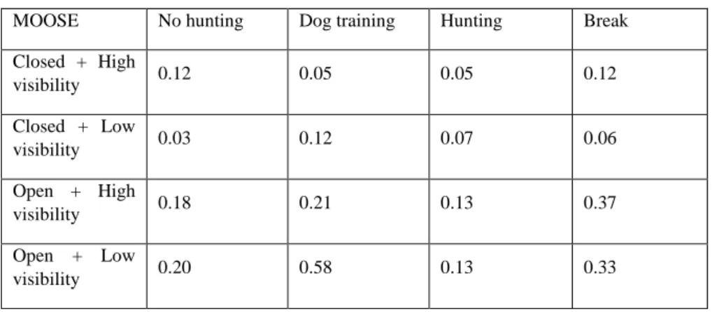
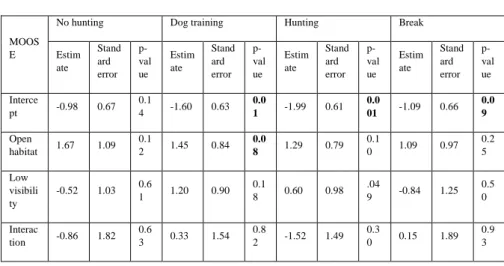
Considering a perfect detection from the cameras, I calculated naïve occupancy and found that moose the highest naïve occupancy is found during the dog training period in the open areas with low visibility (see table 2.A). When testing the linear models for the naïve occupancy a tendency for the same pattern is observed, moose is found more in open forest during the dog training period (see table 2.B, LM, F=1.45, p=0.08).

Table 2. Tables with the results from the naïve occupancy calculations (2.A) and the results of the linear models applied to the naïve occupancy results (2.B) for moose.

2.A

MOOSE No hunting Dog training Hunting Break

Closed + High visibility 0.12 0.05 0.05 0.12 Closed + Low visibility 0.03 0.12 0.07 0.06 Open + High visibility 0.18 0.21 0.13 0.37 Open + Low visibility 0.20 0.58 0.13 0.33

(22)

2.B

MOOS E

No hunting Dog training Hunting Break

Estim ate Stand ard error p-val ue Estim ate Stand ard error p-val ue Estim ate Stand ard error p-val ue Estim ate Stand ard error p-val ue Interce pt -0.98 0.67 0.1 4 -1.60 0.63 0.0 1 -1.99 0.61 0.0 01 -1.09 0.66 0.0 9 Open habitat 1.67 1.09 0.1 2 1.45 0.84 0.0 8 1.29 0.79 0.1 0 1.09 0.97 0.2 5 Low visibili ty -0.52 1.03 0.6 1 1.20 0.90 0.1 8 0.60 0.98 .04 9 -0.84 1.25 0.5 0 Interac tion -0.86 1.82 0.6 3 0.33 1.54 0.8 2 -1.52 1.49 0.3 0 0.15 1.89 0.9 3

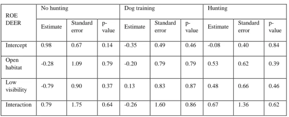
For roe deer, the highest value of naïve occupancy was found in open areas with low visibility during the hunting season (see table 3.A), but any significant result was found to this or any other tendency when analysing with a linear model (see table 3.B).

Table 3. Tables with the results from the naïve occupancy calculations (3.A) and the results of the linear models applied to the naïve occupancy results (3.B) for roe deer.

3.A

ROE DEER No hunting Dog training Hunting

Closed + High visibility 0.40 0.33 0.19 Closed + Low visibility 0.20 0.40 0.25 Open + High visibility 0.40 0.33 0.26 Open + Low visibility 0.33 0.33 0.45

(23)

3.B

ROE DEER

No hunting Dog training Hunting

Estimate Standard error p-value Estimate Standard error p-value Estimate Standard error p-value Intercept 0.98 0.67 0.14 -0.35 0.49 0.46 -0.08 0.40 0.84 Open habitat -0.28 1.09 0.79 -0.20 0.79 0.79 0.53 0.62 0.39 Low visibility -0.79 0.90 0.37 0.13 0.83 0.87 0.48 0.66 0.46 Interaction 0.79 1.75 0.64 -0.26 1.60 0.86 0.67 1.36 0.62

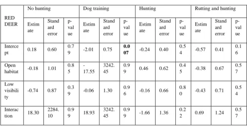
For red deer, the highest values of naïve occupancy were found for open areas with low visibility during the dog training season, and in open areas with high visibility during the hunting season (see table 4.A), but any significant result was found to these or any other tendency when analysing with a linear model (see table 4.B).

Table 4. Tables with the results from the naïve occupancy calculations (4.A) and the results of the linear models applied to the naïve occupancy results (4.B) for red deer.

4.A

RED DEER No hunting Dog training Hunting Rutting +

Hunting Closed + High visibility 0.14 0.09 0.16 0.28 Closed + Low visibility 0.10 0.10 0.12 0.17 Open + High visibility 0.18 0 0.33 0.20 Open + Low visibility 0.26 0.33 0.04 0.18

(24)

4.B

RED DEER

No hunting Dog training Hunting Rutting and hunting

Estim ate Stand ard error p-val ue Estim ate Stand ard error p-val ue Estim ate Stand ard error p-val ue Estim ate Stand ard error p-val ue Interce pt 0.18 0.60 0.7 9 -2.01 0.75 0.0 07 -0.24 0.40 0.5 4 -0.57 0.41 0.1 6 Open habitat -0.18 1.01 0.8 5 -17.55 3242. 45 0.9 9 0.46 0.62 0.4 5 -0.38 0.67 0.5 7 Low visibili ty -0.74 0.87 0.3 9 -0.06 1.30 0.9 6 -0.16 0.66 0.8 0 -0.43 0.71 0.5 4 Interac tion 18.30 2284. 10 0.9 9 18.93 3242. 45 0.9 9 -1.66 1.36 0.2 2 0.69 1.24 0.5 7

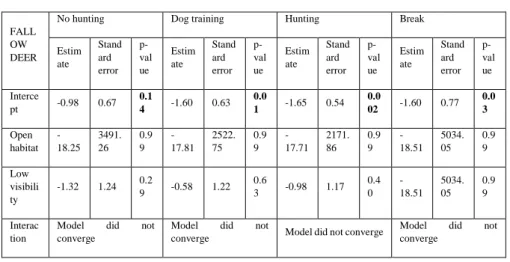
For fallow deer, the highest values of naïve occupancy were found for closed areas with high visibility during the periods of no hunting and dog training (see table 5.A), but any significant result was found to these or any other tendency when analysing with a linear model (see table 5.B). When including the interaction, the models for all seasons did not converge.

As fallow deer are highly localized in the peninsula, and they were not recorded in any of the open forest sites, I did not consider them in any further analysis. After determining the passage rates and naïve occupancy of fallow deer, I decided to exclude this species from further analysis.

Table 5. Tables with the results from the naïve occupancy calculations (5.A) and the results of the linear models applied to the naïve occupancy results (5.B) for fallow deer.

5.A FALLOW

DEER No hunting Dog training Hunting Break

Closed + High visibility 0.10 0.11 0.09 0.08 Closed + Low visibility 0.01 0.03 0.02 0 Open + High visibility 0 0 0 0 Open + Low visibility 0 0 0 0

(25)

5.B

FALL OW DEER

Estim ate Stand ard error p-val ue Estim ate Stand ard error p-val ue Estim ate Stand ard error p-val ue Estim ate Stand ard error p-val ue Interce pt -0.98 0.67 0.1 4 -1.60 0.63 0.0 1 -1.65 0.54 0.0 02 -1.60 0.77 0.0 3 Open habitat -18.25 3491. 26 0.9 9 -17.81 2522. 75 0.9 9 -17.71 2171. 86 0.9 9 -18.51 5034. 05 0.9 9 Low visibili ty -1.32 1.24 0.2 9 -0.58 1.22 0.6 3 -0.98 1.17 0.4 0 -18.51 5034. 05 0.9 9 Interac tion

Model did not converge

Model did not

converge Model did not converge

Occupancy models

I built one model per species and hunting period which includes the site covariate of visibility in the detection and occupancy probabilities, the site covariate of openness in the occupancy probability, and the observational covariate of camera effort in the detection probability. The interaction between the two site covariates was tested, except when the model did not converge. In table 6 the values for the estimates, standard error and p-value are shown to reflect the fitness of each model.

Moose were detected significantly more in the low visibility sites during the hunting period (see table 6.A, F=-0.26, p=0.002). There is a trend for roe deer to be less detected in the low visibility areas during the no hunting period (table 6.B, F=-0.90, p=0.06). In the case of roe deer, effort was significantly positive related to detection (table 6.B, F=0.51, p=0.02). Red deer was significantly less detected in the low visibility sites during the hunting and rutting period (table 6.C, F=-1.76, p=0.005).

Table 6. Parameters of the detection and occupancy probability in which the values of the estimate, standard error and p-value are indicated for every model.

(26)

6.A MOOSE Model: P (effort + Visibility). ᴪ(Openness * Visibility)

No Hunting period Dog training period Hunting period

Estima te Standa rd Error p-valu e Estima te Standa rd Error p-valu e Estima te Standa rd Error p-value Occupan cy Intercept -0.77 0.73 0.29 -0.93 0.78 0.23 0.13 1.02 0.89 Open habitat 1.97 1.48 0.18 1.87 1.32 0.15 8.79 91.73 0.92 Low visibility -0.45 1.15 0.69 1.55 1.41 0.27 -1.35 1.22 0.26 Interacti on -1.09 2.19 0.61 7.03 63.84 0.91 -9.05 91.73 0.92 Detectio n Intercept -2.83 35.31 0.93 -1.10 0.50 0.02 -2.13 0.39 5.84 E-08 Effort 4.89 71.44 0.94 0.08 0.25 0.74 0.12 0.26 0.64 Low visibility -0.26 0.91 0.77 0.11 0.66 0.86 2.12 0.70 0.002 6.B ROE DEER Model: P (effort + Visibility). ᴪ(Openness * Visibility)

No Hunting period Dog training period No hunting period

Estima te Standa rd Error p-valu e Estima te Standa rd Error p-valu e Estima te Standa rd Error p-valu e Occupan cy Intercept 1.02 0.70 0.14 2.68 5.39 0.62 0.09 0.44 0.83 Open habitat -0.29 1.13 0.79 4.80 49.31 0.92 0.59 0.71 0.40 Low visibility -0.59 1.01 0.56 -2.09 5.53 0.70 0.40 0.71 0.57 Interacti on 0.92 2.07 0.65 -4.98 49.33 0.92 0.82 1.70 0.62 Detectio n Intercept 0.28 0.28 0.32 -0.63 0.45 0.16 -0.60 0.21 0.00 4 Effort 0.51 0.23 0.02 0.68 0.47 0.15 0.45 0.29 0.11 Low visibility -0.90 0.48 0.06 0.98 1.28 0.44 0.35 0.32 0.27

(27)

6.C RED DEER Model: P (effort + Visibility). ᴪ(Openness * Visibility)

No hunting period Dog training period Hunting period Hunting and rutting period Est im ate Stan dard Erro r p-valu e Esti mate Sta nda rd Err or p-valu e Esti mat e Stan dard Erro r p-valu e Esti mat e Stan dard Erro r p-val ue Occ upan cy Interc ept 2.1 7 3.46 0.53 8.34 162 0.95 0.4 7 0.64 0.45 0.02 0.48 0.9 5 Open habitat 8.0 4 31.4 8 0.79 2.08 359 0.99 0.7 9 1.09 0.46 -0.71 0.72 0.3 2 Low visibil ity -2.2 3 3.57 0.53 2.64 357 0.99 0.0 6 1.54 0.96 5.18 15.4 5 0.7 3 Intera ction

-2.3 0

1.94 0.23 Model did not converge Dete ction Interc ept -1.6 4 0.41 7.31 E-05 -2.04 0.47 1.81 E-05 -0.7 5 0.31 0.01 0.22 0.46 0.6 2 Effort 0.4 4 0.31 0.15 -0.11 0.32 0.72 0.2 9 0.23 0.21 0.64 0.30 0.0 3 Low visibil ity 0.4 4 0.61 0.46 0.45 0.74 0.54 -0.5 0 0.92 0.58 -1.76 0.63 0.0 05

Passage rates

The weekly passage rates showed the number of passages for each species and hunting period per operating camera in each of the four habitat types.

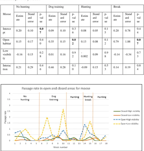
When analysing the passage rate for moose, I found significantly higher passage rate during the dog training period (table 7, GLM, F=0.35, p=0.02), and same trend during the hunting break period (table 7, GLM, F=0.79, p=0.07). In figure 4 we can observe these differences between the open and closed sites between the periods of dog training and hunting break, and any differences between habitats during the hunting period. We can also observe a slightly higher passage rates for the open habitats during the no hunting period, especially at the beginning, but any significant result could confirm this.

(28)

Table 7. Parameters from the generalized linear model performed for moose passage rates during each period in which the values of the estimate, standard error and p-value are indicated for every model.

Moose

Estim ate Stand ard error p-val ue Estim ate Stand ard error p-val ue Estim ate Stand ard error p-val ue Estim ate Stand ard error p-val ue Interce pt 0.20 0.10 0.0 7 0.09 0.10 0.3 6 0.08 0.05 0.1 5 0.20 0.78 0.4 4 Open habitat 0.15 0.17 0.4 0 0.35 0.15 0.0 2 0.13 0.08 0.1 2 0.79 1.88 0.0 7 Low visibili ty -0.16 0.15 0.2 8 0.01 0.16 0.9 2 -0.002 0.09 0.9 8 -0.14 -0.34 0.7 3 Interac tion 0.21 0.29 0.4 6 0.46 0.28 0.1 0 -0.09 0.15 0.5 3 0.14 0.19 0.8 4

Figure 4: Graph showing the passage rate of closed forest with high visibility (green line), closed forest with low visibility (orange line), open forest with high visibility (blue dashed line) and open forest with low visibility (yellow dashed line) habitat per week for moose. Passage rates are calculated as the number of passages for each species and hunting period per operating camera in each habitat type. Each orange line marks the limit between hunting periods.

Any trend or significant result was found for roe deer. When plotting the passage rates per week (figure 5) it is possible to observe a high peak during the third week of the no hunting period in the open areas with high visibility.

(29)

Table 8. Parameters from the generalized linear model performed for roe deer passage rates during each period in which the values of the estimate, standard error and p-value are indicated for every model.

Roe deer

No hunting Dog training Hunting Estimat e Standar d error p-valu e Estimat e Standar d error p-valu e Estimat e Standar d error p-valu e Intercept 0.83 0.36 0.03 0.91 0.42 0.04 0.33 0.15 0.03 Open habitat 0.79 0.61 0.20 0.13 0.68 0.84 0.27 0.24 0.25 Low visibility -0.50 0.51 0.33 -0.13 0.72 0.85 0.20 0.25 0.43 Interactio n -0.72 1.00 0.47 -0.57 1.36 0.67 0.07 0.44 0.87

Figure 5: Graph showing the passage rate of closed forest with high visibility (green line), closed forest with low visibility (orange line), open forest with high visibility (blue dashed line) and open forest with low visibility (yellow dashed line) habitat per week for roe deer. Passage rates are calculated as the number of passages for each species and hunting period per operating camera in each habitat type. Each orange line marks the limit between hunting periods.

For red deer I could find a trend that they have a higher passage rate in open sites during the hunting season (table 9, GLM, F=0.53, p=0.08). Taking this trend into account, if we observe the graph for the passage rate per week (figure 6), we can observe that during the hunting season, this rate is definitely higher in the open areas with high visibility than in the open sites with low visibility and both closed forest sites.

(30)

Table 9. Parameters from the generalized linear model performed for red deer passage rates during each period in which the values of the estimate, standard error and p-value are indicated for every model.

Red deer

No hunting Dog training Hunting Rutting and hunting

Estim ate Stand ard error p-val ue Estim ate Stand ard error p-val ue Estim ate Stand ard error p-val ue Estim ate Stand ard error p-val ue Interce pt 0.27 0.09 0.0 07 0.11 0.09 0.2 4 0.39 0.19 0.0 4 0.44 0.21 0.0 4 Open habitat -0.006 0.15 0.9 6 -0.11 0.15 0.4 6 0.53 0.30 0.0 8 0.28 0.33 0.3 9 Low visibili ty -0.14 0.13 0.2 8 0.10 0.16 0.5 3 -0.14 0.31 0.6 5 -0.14 0.35 0.6 9 Interac tion 0.34 0.25 0.1 8 0.22 0.31 0.4 7 -0.61 0.55 0.2 7 -0.19 0.61 0.7 5

Figure 6: Graph showing the passage rate of closed forest with high visibility (green line), closed forest with low visibility (orange line), open forest with high visibility (blue dashed line) and open forest with low visibility (yellow dashed line) habitat per week for red deer. Passage rates are calculated as the number of passages for each species and hunting period per operating camera in each habitat type. Each orange line marks the limit between hunting periods.

(31)

Discussion

In this study I compared the habitat preference of four ungulate species between open and closed forest habitats with a high or low visibility due to understorey vegetation, during the periods of no hunting, training of hunting dogs, hunting, and hunting with rutting period and break during hunting period. The main conclusion extracted from this study is that in this ungulate multispecies system animals have a different behaviour when considering their habitat selection, meaning that a species-specific management is needed. With the obtained results I found habitat selection patterns for three of the studied species. I can conclude that in this area moose did show a preference for open sites outside the hunting season, during the periods of dog training and hunting break, and showing no difference between habitats during the hunting season. Considering the hunting for fear theory, current hunting practices would work for this species in these regions if we want to remove moose from the open areas during these two periods.

Taking into account the habitat characteristic of openness I found some significant patterns for the studied species. When observing the results obtained, moose showed a significant selection for open habitats during the dog training period and a trend towards the same habitat type during the hunting break when analysing the passage rates data. In the analysis of the naïve occupancy data I could find the same trend of moose selecting the open habitats during the dog training season. Moose selected open habitats during the period of break during hunting, this coincides with my initial hypothesis that outside the hunting season ungulates would prefer open sites (McLoughlin et al. 2011; Lone et al. 2014; Gehr et al. 2017). If this difference had been due to rutting behaviour we would have expected an increase in all habitats in the same way, and not a selection of one habitat in particular, as moose increases its activity during this period (Neumann & Ericsson 2018). Moose has been the only species that partly responded to hunting following the initial hypothesis, as it did select for open sites during two of the periods outside the hunting season, but I expected a higher perception of risk during the dog training period when compared to the no hunting period. This result lead to the conclusion that training of dogs do not affect moose in the same way as when they are hunted, and this period should be considered more similar to no hunting than to hunting period. One explanation why only moose is reacting to hunting is due to the fact that, based on the data from the hunting bags (appendix 3), they are the species with the highest hunting pressure in the area of study, and they do feel a higher hunting risk than the other species. On the contrary, red deer showed a trend to select open habitats during the hunting season, and not showing any significant preference during the other periods. This result could be explained by the increased food quantity in the open areas (Kuijper et al. 2009) and the feeding strategy of red deer, as they

(32)

are intermediate feeders (Hofmann 1989; Gebert & Verheyden-Tixier 2001), which could mean that regardless the hunting pressure, they select for their most suitable feeding areas.

Regarding the habitat characteristic of visibility, I could find patterns for moose, roe deer and red deer when analysing the data obtained from the occupancy models. Moose were significantly found to select more low visibility sites during the hunting season. This coincides with my initial hypothesis that low visibility sites will offer a lower risk of predation to ungulates, making them to prefer significantly more sites with a dense understorey (Lone et al. 2014). I found a tendency that detection probability decreases in the sites with low visibility for roe deer. This result could be due to a detection issue of the cameras when located in denser vegetation, as in the case for low visibility sites. Another possibility could be explained by the fact that animals with a smaller body mass have a smaller effective detection distance from the camera than animals with a larger body mass (Hofmeester et al. 2017), as roe deer is the smallest ungulate considered, could be due to this effect that it has a smaller detection probability. Red deer were significantly found to select less low visibility areas during the hunting and rutting period. One explanation for this result could be that as this species has an intermediate feeding strategy, they are able to feed in areas with less understorey and increase their food intake to prepare for rutting and winter (Gebert & Verheyden-Tixier 2001).

I hypothesized that during the dog training period ungulates would have the same habitat choice than during the hunting period, preferring low visibility sites to decrease risk perception. My results did not confirm this hypothesis, as I did not find any significant result regarding visibility during this time period. In the case of moose I did find that when analysing their passage rate and naïve occupancy there is a preference for open sites during this period, which contradicts my predictions. Open sites offer a less protection feeling for ungulates (Benhaiem et al. 2008), and the effect of dogs training in the area should give a higher risk perception (Cromsigt et al. 2013) and make them select towards closed habitats with low visibility. This indicates that the effect of dogs is lower than I firstly expected, and that they are not affected by dogs targeting other species, as this does not give ungulates a risk perception in the same way as hunting for this species. Future studies could focus in different disturbances produced by dogs, analysing differently the following periods: period in which dogs that target other species are being trained in the area, dogs used to hunt other species are being used in the area, dogs that target the studied species are being trained in the area, and separating the hunting period between the moment in which dogs are allowed to hunt the studied species and when they are not.

(33)

Regarding the data obtained for fallow deer in this study, my results show passages only in closed forest areas, which can lead to the conclusion that this species select deliberately this type of habitat. Based on the knowledge I have gathered from the study area, this conclusion is not likely to be true. Fallow deer in the Järnäshalvön peninsula have a limited distribution, and they have been found to aggregate in the southernmost part, where there are a few agricultural lands. Liberg & Wahlström (1995) found that fallow deer have an innate reluctance to disperse, and they are restricted to the surroundings where they were initially released. This leads to a high variability in their distribution, with high densities in some locations, and almost no individuals in the rest of areas (Liberg & Wahlström 1995), as we have seen in this study. A larger amount of cameras are located in closed forest, which could also be a reason why we find them in closed sites. In order to have a better knowledge of the habitat selection of this species, I would need a more targeted camera trapping distribution, including also agricultural fields where, for the information obtained from the area, we know they spend an important amount of time.

In this study I used three different methods to assess the habitat preference of these ungulate species. Occupancy modelling is a method that is been highly used in camera trap studies. Its best advantage is that with this type of model you can determine the detection probability of the cameras, and account for the fact that this probability differs among them. In my study this type of model did not show the same tendency as the others showed. Passage rate and naïve occupancy assume a perfect detection from the cameras and its results should be interpreted with caution. On the other hand, running a separate model per species and period already corrected for differences between periods within species, which improves the reliability of comparisons within species more.

There is evidence of a general increase in ungulate populations in Europe which can lead to an increase in human-wildlife conflicts (Apollonio, Andersen & Putman, 2010; Cromsigt et al. 2013). This trend shows the need to improve the knowledge of these animals at a small scale, to be able to introduce useful management actions in controlling ungulate populations. Hunting can induce changes in ungulate population trends directly, by reducing the number of individuals, or indirectly, by increasing the feeling of risk of being predated and decreasing their fitness by moving to less risky areas with lower quality food (Neumann, Ericsson & Dettki 2009). This is the base of hunting for fear strategy (Cromsigt et al. 2013), a strategy to increase risk perception in ungulate populations to remove them from those systems degraded by their herbivory pressure. Based on my results we can see that moose does select open habitat sites outside of the hunting season, but that they do not select differently any habitat type during the

(34)

hunting season. This is an evidence that moose do react to hunting in terms of habitat selection. When comparing the hunting intensity in the area we can see that moose is the most hunted species, which can be a reason why they are the only species reacting to hunting in terms of habitat selection in the area. Roe deer and red deer from this area would need a higher pressure from hunting to react to it and select their habitat to avoid it. In this case there is potential to implement the strategy of hunting for fear, increasing hunting pressure and forcing ungulate populations to move towards those areas that will be less or not degraded by their foraging pressure. It is important to point out that results from this study show that ungulates do react differently to hunting pressure, and in a multi-species system as the Järnäshalvön peninsula, species specific management is needed.

(35)

Acknowledgements

First of all I would like to thank Tim for all his unconditional support, incredibly amount of hours spent discussing and also his endless patience dealing with all my R troubles. Also to show me motivation and passion for the job I did, as well as for becoming a role model as a researcher to be able to combine infinite projects with being a musician with high programming skills. Thanks for being one of the main supports from the beginning.

Thanks to Joris for his support, useful comments and all the information and advice to learn how to write and organize a scientific report. Thanks also to my supervisor from in Wageningen University and Research Patrick Jansen to help me and make possible for me to come to Umeå to do this project.

Also special thanks to Navinder to share his R knowledge and constant support, to Wiebke for her highly useful advice and information, to Sonya and the rest of field technicians that made this study possible, and all the people from the department that made me feel really comfortable during my stay. Also, special thanks to Fredrik for being my examiner and spending time reading my thesis.

Thanks to my family, especially the one in Umeå, Marta and Martí to share your home with me, really good memories that I will never forget, and special thanks for bringing my nephew Blai, I will never forget how I could share your first months of life.

To my side by side warrior Sherry, with whom I shared every good and less good moments of this thesis, you have been an important support in this experience. I am really glad to finish this project with not a colleague but a friend with whom I know will live many more experiences side by side. Good luck in your career as a researcher, I will miss your bun across the computer every morning, but I am sure you will succeed in every step you make.

Thanks to all my friends back home, for still giving their support even from the distance. Also thanks to my friends in Wageningen specially my housemates and family from Poststraat. Thanks to Cris, without you I would have never come here to do this thesis, thanks for all the love we share in what we do and all the fun moments. Finally, thanks to all master students with whom I shared the room, sharing lots of good moments and some misery, especially to Shoumo, Freja and Björn. Thanks to the Fellowship and Josefin for all the good moments together, to Mark and Jorina for their help and advice during my struggling times with R, and special thanks to Henrik for listening and sharing his positivity and time, there is no problem that cannot be solved with a good break.

(36)

Literature cited

Apollonio, M., Andersen, R., & Putman, R. (Eds.). (2010). European ungulates and their management in the 21st century. Cambridge University Press.

Benhaiem, S., Delon, M., Lourtet, B., Cargnelutti, B., Aulagnier, S., Hewison, A. M., Morellet, N. & Verheyden, H. (2008). Hunting increases vigilance levels in roe deer and modifies feeding site selection. Animal Behaviour, 76(3), 611-618.

Bonnot, N., Morellet, N., Verheyden, H., Cargnelutti, B., Lourtet, B., Klein, F., & Hewison, A. M. (2013). Habitat use under predation risk: hunting, roads and human dwellings influence the spatial behaviour of roe deer. European journal of wildlife research, 59(2), 185-193.

Bouyer, Y., Rigot, T., Panzacchi, M., Moorter, B. V., Poncin, P., Beudels-Jamar, R., Odden, J., & Linnell, J. D. (2015, April). Using zero-inflated models to predict the relative distribution and abundance of roe deer over very large spatial scales. Annales Zoologici Fennici (Vol. 52, No. 1–2, pp. 66-76). Finnish Zoological and Botanical Publishing.

Brown, J. S., Laundré, J. W., & Gurung, M. (1999). The ecology of fear: optimal foraging, game theory, and trophic interactions. Journal of Mammalogy, 80(2), 385-399.

Bubnicki, J. W., Churski, M., & Kuijper, D. P. (2016). TRAPPER: An open source web‐based application to manage camera trapping projects. Methods in Ecology and Evolution, 7(10), 1209-1216.

Burton, A. C., Neilson, E., Moreira, D., Ladle, A. , Steenweg, R. , Fisher, J. T., Bayne, E. , Boutin, S. and Stephens, P. (2015), REVIEW: Wildlife camera trapping: a review and recommendations for linking surveys to ecological processes. Journal of Applied Ecology, 52: 675-685. doi:10.1111/1365-2664.12432

Cromsigt, J. P., Kuijper, D. P., Adam, M., Beschta, R. L., Churski, M., Eycott, A., Kerley, G. I. H., Mysterud, A., Schmidt, K., & West, K. (2013). Hunting for fear: innovating management of human–wildlife conflicts. Journal of Applied Ecology, 50(3), 544-549.

Ericsson, G., Neumann, W., & Dettki, H. (2015). Moose anti-predator behaviour towards baying dogs in a wolf-free area. European journal of wildlife research, 61(4), 575-582.

(37)

Fiske, I. & R. B. Chandler. 2011. unmarked: An R package for fitting hierarchical models of wildlife occurrence and abundance. Journal of Statistical Software 43:1–23

Gebert, C. & Verheyden‐Tixier, H. (2001), Variations of diet composition of Red Deer (Cervus elaphus L.) in Europe. Mammal Review, 31: 189-201. doi:10.1111/j.1365-2907.2001.00090.x

Gehr, B., Hofer, E. J., Pewsner, M., Ryser, A., Vimercati, E., Vogt, K., & Keller, L. F. (2018). Hunting‐mediated predator facilitation and superadditive mortality in a European ungulate. Ecology and evolution, 8(1), 109-119.

Hofmann, R. R. (1989). Evolutionary steps of ecophysiological adaptation and diversification of ruminants: a comparative view of their digestive system. Oecologia, 78(4), 443-457.

Hofmeester, T. R., Rowcliffe, J. M., Jansen, P. A., Williams, R. and Kelly, N. (2017), A simple method for estimating the effective detection distance of camera traps. Remote Sensing in Ecology and Conservation, 3: 81-89. doi:10.1002/rse2.25

Kindbladh, N. (2015). Timing of the rut in fallow deer (Dama dama) (MSc dissertation). Accession No. 2015:21. Swedish University of Agricultural Sciences.

Kuijper, D.P., Cromsigt, J.P.G.M., Churski, M., Adam, B., Jędrzejewska, B. & Jędrzejewski, W., (2009). Do ungulates preferentially feed in forest gaps in European temperate forest?. Forest Ecology and Management, 258(7), pp.1528-1535.

Kuijper, D. P. J. (2011). Lack of natural control mechanisms increases wildlife–forestry conflict in managed temperate European forest systems. European Journal of Forest Research, 130(6), 895.

Lavsund, S., Nygén. T., & Solberg, E.J. (2003) Status of moose populations and challenges to moose management in Fennoscandia. Alces 39:109-130.

Liberg, O., & Wahlström, K. (1995). Habitat stability and litter size in the Cervidae; a comparative analysis. Wahlström K, Natal dispersal in roe deer. Doctoral thesis, Stockholm University, Stockholm.

Lone, K., Loe, L. E., Gobakken, T., Linnell, J. D., Odden, J., Remmen, J. and Mysterud, A. (2014), Living and dying in a multi‐predator landscape of fear: roe deer are squeezed by contrasting pattern of predation risk imposed by lynx and humans. Oikos, 123: 641-651.

(38)

MacKenzie, D. I. & Royle, J. A. (2005), Designing occupancy studies: general advice and allocating survey effort. Journal of Applied Ecology, 42: 1105-1114. doi:10.1111/j.1365-2664.2005.01098.x

MacKenzie, D. I., Nichols, J. D., Royle, J. A., Pollock, K. H., Bailey, L. L., & Hines, J. E. (2006). Occupancy estimation and modeling: inferring patterns and dynamics of species occurrence. Academic Press. Burlington MA.

McLoughlin, P. D., Vander Wal, E., Lowe, S. J., Patterson, B. R., & Murray, D. L. (2011). Seasonal shifts in habitat selection of a large herbivore and the influence of human activity. Basic and Applied Ecology, 12(8), 654-663.

Neumann, W., Ericsson, G., & Dettki, H. (2009). The non-impact of hunting on moose Alces alces movement, diurnal activity, and activity range. European Journal of Wildlife Research, 55(3), 255-265.

Neumann, W. & Ericsson, G. (2018). Influence of hunting on movements of moose near roads. The journal of wildlife management, 82: 918-928.

doi:10.1002/jwmg.21448.

Niedballa, J. , Sollmann, R. , Courtiol, A. , Wilting, A. & Jansen, P. (2016), camtrapR: an R package for efficient camera trap data management. Methods in Ecology and Evolution, 7: 1457-1462. doi:10.1111/2041-210X.12600 Pfeffer, S. (2016). Evaluation of ungulate population densities based on three different methods in the Nordmaling area (Västerbotten, Sweden) (MSc dissertation). Swedish University of Agricultural Sciences.

Proffitt, K. M., Grigg, J. L., Hamlin, K. L., & Garrott, R. A. (2009). Contrasting effects of wolves and human hunters on elk behavioral responses to predation risk. Journal of Wildlife Management, 73(3), 345-356.

Rowcliffe, J. M., Carbone, C., Jansen, P. A., Kays, R., & Kranstauber, B. (2011). Quantifying the sensitivity of camera traps: an adapted distance sampling approach. Methods in Ecology and Evolution, 2(5), 464-476.

Vavra, M., & Riggs, R. A. (2010). Managing multi-ungulate systems in disturbance-adapted forest ecosystems in North America. Forestry, 83(2), 177-187.

Wilmshurst, J.F., Fryxell, J.M., 1995. Patch selection by Red deer in relation to energy and protein-intake—a reevaluation of Langvatn and Hanley (1993) results. Oecologia 104, 297–300.

(39)

Appendix

Appendix 1

Table comprising the exact initial and end dates considered per each period analysed per species in this study.

No hunting Dog training Hunting Rutting and hunting Start date End date Start date End date Start date End date Start date End date Moo se 01/07 /17 31/07 /17 01/08 /17 03/09 /17 04/09 /17 25/09 /17 09/10 /17 31/10 /17 Roe deer 01/07 /17 31/07 /17 01/08 /17 15/08 /17 16/08 /17 31/10 /17 Red deer 01/07 /17 31/07 /17 01/08 /17 15/08 /17 16/08 /17 31/08 /17 _01/09 /17 30/09 /17 01/10 /17 31/10 /17 Fall ow deer 01/07 /17 31/07 /17 _01/08 /17 31/08 /17 01/09 /17 20/10 /17 21/10 /17 31/10 /17

(40)

Appendix 2

Graph showing the number of sequences taken each month of the whole year of study per each species. A total number of 227 sequences were recorded per moose, with a maximum of 44 in October of 2017. For red deer, 395 sequences were recorded in total, with a maximum in September 2017 of 79 sequences. 579 sequences were recorded for roe deer with a maximum of 121 in July of 2017. Lastly, a total number of 101 sequences were recorded for fallow deer with its maximum in August 2017 with 26 sequences.