Results of a field study on a driver distraction warning system

(1)

VTI rapport 639A Published 2009

www.vti.se/publications

Results of a field study on a driver distraction

warning system

Katja Kircher Albert Kircher Christer Ahlström

(2)

(3)

Publisher: Publication: 639A Published: 2009 Project code: 40658 Dnr: 2006/0226-26

SE-581 95 Linköping Sweden Project:

IVSS Distraction and Drowsiness

Author: Sponsor:

Katja Kircher, Albert Kircher and Christer Ahlström Saab, within IVSS programme

Title:

Results of a field study on a driver distraction warning system

Abstract (background, aim, method, result) max 200 words:

The main goal of the distraction and drowsiness field study was to evaluate a system for detecting driver distraction and drowsiness. This report focuses on the results of the study, indicating how a distraction warning system influenced glance behaviour.

A vehicle was instrumented with an automatic eye tracker and other sensors. Seven participants drove the vehicle during one month each. During the first ten days a baseline was collected. Afterwards the warnings were activated, which involved that the drivers received a vibration in the seat when the algorithm determined that they had looked away from the forward roadway for a too long time. The main finding was that the drivers’ gaze behaviour was not influenced much by the distraction warnings. The drivers received distraction warnings at about the same frequency during the treatment and the baseline phase. Performance indicators like “percent road centre” and others did not change from baseline to treatment phase. The average percentage of very long glances decreased slightly in the

treatment phase, suggesting that the warning had an effect on the more extreme glance behaviour. There are also indications that the system helped prevent further extended glances away from the road

immediately after a warning was issued.

Keywords:

distraction, field study, eye tracking, drowsiness

(4)

Utgivare: Publikation: 639A Utgivningsår: 2009 Projektnummer: 40658 Dnr: 2006/0226-26 581 95 Linköping Projektnamn:

IVSS Distraktion och sömnighet

Författare: Uppdragsgivare:

Katja Kircher, Albert Kircher och Christer Ahlström Saab, inom IVSS-programmet

Titel:

Resultat av en studie av distraktionsvarningssystems påverkan på förarnas blickbeteende

Referat (bakgrund, syfte, metod, resultat) max 200 ord:

Huvudmålet med distraktions- och sömnighetsstudien var att utvärdera ett system för att detektera förar-distraktion och sömnighet. Denna rapport fokuserar på studiens resultat, huruvida ett förar- distraktionsvar-ningssystem påverkade förarnas blickbeteende.

En försöksbil utrustades med en automatisk "eye tracker" och andra sensorer. Sju deltagare körde fordonet under en månad var. Under de första tio dagarna samlades data om vanligt körbeteende utan varningssystem (baseline). Sedan aktiverades varningarna, vilket innebar att förarna fick en varning i form av en vibration i förarsätet när algoritmen bedömde att de hade tittat bort från vägen för länge. Huvudresultatet var att förarnas blickbeteende inte förändrades mycket på grund av distraktionsvarnings-systemet. Förarna fick distraktionsvarningar med ungefär samma frekvens när varningarna var på som under baseline-fasen. Prestationsindikatorer som ”percent road centre” och liknande ändrades inte heller mellan baseline-fasen och när varningarna var på. Den genomsnittliga procentandelen av långa blickar bort sjönk något när varningarna var på, vilket innebär att varningarna hade en effekt på det mer extrema blickbeteendet. Det finns även tecken på att varningarna förhindrade fortsatta längre blickar bort från vägen precis efter en varningsaktivering.

Nyckelord:

distraktion, fältstudie, eye tracking, sömnighet

(5)

Preface

This report is the last in a series of three on an extended field study on driver distraction financed by the IVSS programme. The first report (Kircher, K., 2007) covers the theore-tical background of driver distraction with special focus on glance behaviour and traffic safety. The second report (Kircher, K., Kircher, A. & Claezon, F., 2009) describes the instrumented vehicle and the experimental setup in detail. The present report contains the results of the study.

Christer Ahlström, VTI, contributed with a large part of the analyses done in Matlab, and with valuable suggestions and discussion points. Albert Kircher, VTI, provided the chapter on self-reported results and was an important partner for discussions. Without him and Fredrich Claezon (then Saab, now Scania) it would not have been possible to conduct the study.

Special thanks go to Arne Nåbo at Saab for taking us on board, and to the IVSS pro-gramme for financing this study. We would also like to thank SmartEye AB for support with the eye tracker. Last but not least we thank all participants who were willing to share their data with us, and who made this study possible.

Linköping March 2009

(6)

Quality review

Review seminar was carried out on 18th of December 2008 where Astrid Linder reviewed and commented on the report. Katja Kircher has made alterations to the final manuscript of the report. The research director of the project manager Jan Andersson examined and approved the report for publication on 10th of March 2009.

Kvalitetsgranskning

Granskningsseminarium genomfört 2008-12-18 där Astrid Linder var lektör. Katja Kircher har genomfört justeringar av slutligt rapportmanus 2009-03-10. Projektledarens närmaste chef, Jan Andersson, har därefter granskat och godkänt publikationen för publicering 2009-03-10.

(7)

9.1.1 General results 77 9.1.2 Results before driving 78 9.1.3 Results after baseline driving with the system deactivated (“between”) 78 9.1.4 Expectations of the distraction warning system (“between”) 78 9.1.5 Expectations of the drowsiness warning system (“between”) 79 9.1.6 Results after the test period (“after”) 79 9.1.7 Experience with the distraction warning system 79 9.1.8 Experience with the drowsiness warning system 80 9.2 Interviews... 80

9.3 Discussion of self-reported results... 80

10 Difficulties encountered... 82

11 General discussion ... 84

11.1 Method and data treatment... 84

11.2 General results ... 85

11.3 Driver distraction warning system ... 86

11.4 Recommendation for further analyses ... 88

11.5 Ground truth on driver distraction ... 90

11.6 Improvement of the AttenD algorithm ... 91

11.7 Future research ... 93

12 Conclusions ... 94

(9)

Results of a field study on a driver distraction warning system

by Katja Kircher, Albert Kircher and Christer Ahlström

VTI (Swedish National Road and Transport Research Institute) SE-581 95 Linköping Sweden

Summary

An extended field study on driver distraction and drowsiness was conducted in an in-strumented vehicle, which was equipped with an eye tracker and other sensors. This report focuses on the findings concerning driver distraction. Seven participants used the car just as their own car during a period of one month each. During the baseline phase, which comprised of the first ten days of the trial the distraction warnings were deacti-vated. During the treatment phase, consisting of the remaining 20 days, the warnings were activated, meaning that the driver received a vibration in the seat whenever an algorithm called AttenD determined that the driver was distracted from the driving task. The participants’ subjective opinion about the warning systems was assessed with the help of three questionnaires.

The method is promising for driver distraction research, as it investigates naturalistic behaviour in a naturalistic setting. The employed eye tracker held up to the expecta-tions, even though it is recommendable for future research to use more than two cameras. With the current setup, there was a tendency that tracking was lost just when driver distraction occurred. A robust data acquisition system is a requirement.

The main finding was that the drivers’ gaze behaviour was not influenced much by the distraction warnings. The drivers received distraction warnings at about the same frequency during the treatment phase as they would have during the baseline phase. This indicates that they did not avoid the warnings. Performance indicators like “percent road centre” and the newly developed percentage of glances within the “field relevant for driving” did not change from baseline to treatment phase. The standard deviation of gazes did not change, either. The average percentage of very long glances decreased slightly in the treatment phase, suggesting that the warning had an effect on the more extreme glance behaviour. There are also indications that the system helped prevent further extended glances away from the road immediately after a warning was issued. The results from the questionnaire indicate that the drivers were satisfied with AttenD. Their expectations had been positive, and they indicated no disappointment. The drivers stated that they trusted the system, that the warnings were not experienced as disturbing, and that the system made them more aware of what they did while driving. Some

drivers reported using their cell phones less while driving as a consequence of the warnings.

The analyses presented here are of a rather general nature, and more detailed analyses could provide new insights and a more differentiated picture of the usefulness of the driver distraction warning system. It is also important to investigate whether AttenD influenced driving behaviour like speed choice or steering variables.

A general problem with driver distraction research is the absence of a ground truth, which could be used as a benchmark, against which distraction detection algorithms could be compared and evaluated.

(10)

(11)

Resultat av en studie av distraktionsvarningssystems påverkan på förarnas blickbeteende

av Katja Kircher, Albert Kircher och Christer Ahlström VTI

581 95 Linköping

Sammanfattning

Detta är den tredje och sista delen i en rapportserie om förardistraktion. Serien är baserad på en längre fältstudie om trötthet och distraktion i trafiken och denna rapport fokuserar alltså på de resultat som rör distraktion. Sju deltagare använde en instru-menterad bil som utrustats med ett distraktionsvarningssystem kallat AttenD under en månad vardera. De första tio dagarna utgjorde den så kallade “baseline”-fasen, och då var distraktionsvarningssystemet avstängt. Under de resterande 20 dagarna var var-ningssystemet på, vilket innebar att förarsätet började vibrera när distraktionsalgoritmen ansåg att föraren var distraherad från köruppgiften. Försökspersonernas subjektiva upp-fattning av varningssystemet undersöktes med hjälp av tre enkäter.

Den instrumenterade bilen var bland annat utrustad med en datalogger och ett eye tracking-system. Den eye tracker som användes levde upp till förväntningarna även om studien gjordes under tuffa fältförhållanden. Vi rekommenderar dock att fler än två kameror används i framtida studier. Med utrustningen som användes här kunde vi se en tendens att trackingen tappades just när förarna blev distraherade. En annan viktig lär-dom från projektet är att ett stabilt dataloggsystem är ett krav för en fältstudie av denna typ.

Huvudresultatet från studien var att förarnas blickbeteende inte förändrades mycket på grund av distraktionsvarningssystemet. Förarna fick distraktionsvarningar med ungefär samma frekvens när varningarna var på som de skulle ha fått under baseline-fasen. Detta visar att de inte undvek varningarna. Prestationsindikatorer som ”percent road centre” och procentandelen av blickar inom ”field relevant for driving”, som togs fram i denna studie, ändrades inte heller mellan baseline-fasen och när varningarna var på. Standardavvikelsen av blickriktningen förändrades inte heller. Den genomsnittliga procentandelen av långa blickar (mer än 2 sekunder) bort från vägen sjönk något när varningarna var på, vilket innebär att varningarna hade en effekt på det mer extrema blickbeteendet. Det finns även tecken på att varningarna förhindrade fortsatta längre blickar bort från vägen precis efter en varningsaktivering.

Resultaten från enkäterna visar att förarna var nöjda med AttenD. Deras förväntningar på systemet var positiva och de visade ingen besvikelse efter försöksperioden. Förarna uppgav att de litade på systemet, att varningarna inte upplevdes som störande och att de kände att systemet hjälpte dem att bli mer medvetna om vad de höll på med medan de körde. Några förare rapporterade att de använde sina mobiltelefoner mindre under kör-ningen på grund av varningarna.

Analyserna som presenteras här är på en övergripande nivå och mer detaljerade analyser skulle kunna leda till nya insikter och en mer differentierad bild av användbarheten av distraktionsvarningssystemet. Det är också viktigt att undersöka om AttenD påverkade körbeteenden såsom hastighetsval och styrrelaterade parametrar.

(12)

Ett generellt problem med förardistraktionsforskningen är att det saknas en etablerad sanning om vad distraktion egentligen är som skulle kunna användas som mått med vilket distraktionsdetektionsalgoritmer kan jämföras och evalueras.

(13)

1 Introduction and background

This report is the third in a series of three, focusing on the results of the IVSS Inattention and Drowsiness project. The first report in the series covers a literature review on driver distraction with focus on eye gaze behaviour and its relation to driving behaviour and traffic safety (Kircher, K., 2007), the second report gives a detailed description of the method used, including a chapter on “lessons learnt” (Kircher, K., Kircher, A. & Claezon, F., 2009). In order to be able to make most of the present report it is highly recommended to read through the second report, which gives a detailed overview of the method employed in this study. In this report only parts of the method that are immediately necessary for understanding the results are taken up, for details the reader is referred to the other two reports in the series.

The goal of the study was to evaluate a real time distraction mitigation system called AttenD and a drowsiness mitigation system in a long-term field test in a natural setting. Due to the reason that the eye tracker used in the study had not been subjected to this kind of field test before, and that the method used was quite new for all partners in-volved, another goal of the study was to evaluate both the equipment and the method itself.

Simulator studies had shown that it was difficult to attain “true distraction” in an arti-ficial setting (e.g. Almén, 2003; Karlsson, 2005). Distraction mitigation researchers, who performed a series of experiments in different simulators recommend using a field test for further evaluation of distraction mitigation systems (e.g. Donmez, Ng Boyle & Lee, 2006, 2007; Donmez, Ng Boyle, Lee & McGehee, 2006; Zhang & Smith, 2004). These results, together with the maturation of remote eye tracking systems, which can now be operative for a long time without experimenter intervention, led to the decision to perform a distraction mitigation test in the field, using the general methodological setup of a field operational test (FOT), but on a smaller scale than common for this type of test.

Seven drivers used an instrumented Saab 9-3 in their daily lives for about a month each. During the baseline phase, which consisted of the first approximately 10 days, the driver was not given any feedback on his behaviour; the car “behaved” just like a normal car. The driving behaviour, including warnings that would have been given, was logged. During the treatment phase, which lasted for the remaining approximately 20 days, logging continued, and warnings for inattention and drowsiness were not only logged but also given to the driver. The drivers’ subjective opinion about the warning systems and their expectations and experiences were obtained via a set of questionnaires and by interviewing the drivers.

In order to help interpreting the results a short description of the inattention detection algorithm is given here. A more detailed version can be found in (Kircher, K., Kircher, A. & Claezon, F., 2009).

The algorithm AttenD is based on a defined visual vehicle model, which divides the vehicle into different zones like the windshield, the speedometer, the mirrors, the dash-board, etc., and on the time the driver spends glancing at those zones. A buffer is decremented over time when the driver looks away from the “field relevant for driving” (FRD), which consists of the intersection between a circle of a visual angle of 90° and the vehicle windows, excluding the area of the mirrors. When the driver’s glance is inside the FRD, the buffer is incremented again, until a maximum value of 2 s is reached. Special latencies for decrementing are built in for the mirrors and the

(14)

speedo-meter, recognising the need to check mirrors and speedometer for traffic safety reasons. There is a delay of 0.1 s for increasing the buffer again after having been decreased, in order to compensate for focal adaptation and an “adaptation of the mind” to the road scene and away from the secondary task that had been attended. When the buffer reaches zero the driver is considered to be distracted, and when certain further conditions were met, which are described in detail in Kircher et al. (2009), a warning was given to the driver.

The described rules apply as long as gaze direction tracking data of a quality of at least 0.25 is present. Otherwise the algorithm relies on head/nose direction tracking with comparable rules, or, if head/nose tracking is not available either, on a simple decision rule for no-tracking cases, trying to keep false alarms at an acceptable level without missing crucial warnings.

The study was conducted in order to find out whether the distraction warning system AttenD would influence behaviour such that drivers would look away from the FRD less with the system active, which was supposed to increase traffic safety. Several hypotheses are related to this research question. The most immediate effect would be that AttenD cuts off glances away from the forward roadway, making drivers look up faster than they would have without a warning. This question is taken up in Chapter 8. Another effect could be that drivers try to avoid warnings, meaning that the frequency of driver distraction, and thus the number of warnings, decreases with the distraction warning system activated. This issue is addressed in Chapter 4. Furthermore, the amount of very long glances, that are considered to be especially dangerous, might be reduced with a distraction warning system. Glance duration is considered in Chapter 5. Last but not least, a distraction warning system could generally have an effect on how drivers distribute their glances in the environment. They might focus their attention more on the road centre and other areas relevant for driving. This is investigated in Chapter 6.

The report is structured such that for each chapter a short introduction of the topic in question is presented, and after the presentation of the results a short discussion of the topic is included. A more general and comprehensive discussion can be found in the end of the report.

(15)

2 Data

preparation

For each driver both video logs and text logs were available. More detailed descriptions of the log data can be found in Kircher et al. (Kircher, K., Kircher, A. & Claezon, F., 2009). The participants are numbered from 10 to 16, in the chronological order in which they participated in the study.

The text logs came from seven modules. One came from the GPS and included position and speed. The remaining six modules shared a common time stamp and logged a host of data from the sensors installed in the vehicle, and from the CAN. They had the following format in common: The filename consisted of a code for the vehicle, the driver, the module, the day of the year and the time of day when the file was created. All those six log files belonging to the same trip therefore carried the same filename save for the module ID. Examples are presented in Table 1. This nomenclature allowed fast and unambiguous identification of files and trips. The name structure was used when programming analysis code.

Table 1 Examples for filenames from different modules.

Filenames from Module 8050 (IDP) Filenames from Module 8100 (CAN-bus)

da-1-11-8050_071114_233631.log da-1-11-8050_071115_081952.log da-1-11-8050_071115_083747.log da-1-11-8100_071114_233631.log da-1-11-8100_071115_081952.log da-1-11-8100_071115_083747.log

The following six modules existed:

8010: Warning control module (3 variables)

8020: Raw SmartEye data module (21 variables)

8030: Drowsiness module (13 variables)

8050: Inattention Detection Programme (IDP) module (25 variables)

8070: In/Out module (5 variables)

8100: CAN bus data (25 variables)

Therefore, excluding the two video channels and the GPS log, 92 variables were logged continuously, including two time stamps that were equal across all six parallel modules. A more detailed description of exactly which variables were logged in which module can be found in Kircher et al. (Kircher, K., Kircher, A. & Claezon, F., 2009) describing the method of the study.

All six modules shared the time stamp, but the rows for each module were written at slightly different times. This was due to the fact that the modules consisted of separate programmes, which ran in parallel. The operating system Windows determined via a scheduler in which order the processor executed those different programmes. This switching between processes was very fast and therefore execution appeared to be parallel. There was no predetermined order in which the processes were executed, therefore it was not determined either in which order between processes the data rows were written to memory. In general the time delay until the measured data was com-mitted to memory was very short, from around 0.025 s to 0.1 s, depending on the

(16)

module. For analyses that drew on data from different modules the row with the nearest time stamp was considered to be the matching information.

For analysis the data had to be reduced. Several different reduction methods were used. One was trip-based, for more general analysis of driver behaviour, such as length of trip, distribution of speed across the trip and the like. Glance frequency analyses were either based on weighted trip-based data or on absolute counts of glances. Another reduction method was event-based, where each occurrence of inattention as determined by the AttenD algorithm counted as event. This reduction method was mainly used for the reaction time related behaviour and warning frequency.

Matlab code was written for the extraction of relevant data. For some analyses further processing was done in SPSS.

Due to the small number of participants and the large variation between participants with respect to a number of variables, not many inferential tests were done. Where they were done, they were usually kept within participants.

The treatment phase was about twice as long as the baseline phase for most participants. Therefore for most analyses comparisons were not only made between baseline and treatment phase, but the treatment phase was split into three periods of similar duration, as was also done by LeBlanc et al. (2006). This can be seen as a simplified method to account for some time series effects. The exact number of days during which the participants could use the car varied between drivers, therefore the time periods could have slightly different lengths across participants. These periods are called “weeks” or “phases” in the analyses, with week 1 corresponding the baseline condition, week 2 or phase 2 being the first week in the treatment condition, week 3 or phase 3 being the second week in the treatment condition and week 4 or phase 4 being the last week in the treatment condition. An overview of the number of days per week per participant can be found in Table 2. Participant 16 had a somewhat shorter driving period than the other participants, due to approaching summer holidays. For Participant 14 week 2 was inter-rupted, because the project sponsors required the car to be present at a press event. For all analyses except those on trip statistics the first two days of the baseline phase were excluded, because these days were considered to be the period needed to become familiar with the vehicle. The first two days of the treatment phase were excluded, too, because they were considered to be needed to become familiarised with the distraction warning system. All inferential statistics were computed with an alpha level of 0.05.

(17)

Table 2 The number of days in the baseline phase and in the treatment condition per participant (first row), the chronological number of days per phase which were included in each phase (second row), and the total number of days per phase included in the analyses (third row). The first two days in each condition were discarded as adaptation period. Participant Number # days baseline (phase 1) # days treatment (phase 2) # days treatment (phase 3) # days treatment (phase 4) # days treatment total 10 11 (3–11) 9 3–8 6 9–14 6 15–20 6 20 (3–20) 18 11 13 (3–13) 11 3–8 6 9–14 6 15–21 7 21 (3–21) 19 12 13 (3–13) 11 3–8 6 9–14 6 15–21 7 21 (3–21) 19 13 10 (3–10) 8 3–8 6 9–14 6 15–20 6 20 (3–20) 18 14 12 (3–12) 10 3–4; 7–11 7 12–19 8 20–26 7 24 (3–4;7–26) 22 15 10 (3–10) 8 3–8 6 9–14 6 15–21 7 21 (3–21) 19 16 8 (3–8) 6 3–6 4 7–11 5 12–15 4 15 (3–15) 15

(18)

3 Trip

statistics

In this chapter an overview is given of the trip lengths and speed distributions for the different drivers and weeks. For the general trip statistics the first two days of the baseline and treatment phase were not filtered out.

Trip length is calculated based on the logged odometer data. Under normal operation, each time the ignition was switched off for longer than one minute a new log file was generated. Each separate log file is considered as one separate trip, no matter how much time passed between switching off the ignition and switching it on again. Therefore, the maximum trip length is in principle limited by the size of the tank of the car.

For each trip the first logged odometer value was subtracted from the last logged odometer value of the same trip in order to determine the logged distance of the current trip. The last odometer value of the previous trip was also subtracted from the first odometer value of the current trip, which resulted in the distance that was not logged in between those trips. This distance was added to the current trip for the total distance per trip, as it was assumed that in most cases the distance not logged was a result of the booting computer. A number of trips were compared to video recordings for validation of this hypothesis, and it proved to be true for a large majority of trips. However, especially at times when the computer did not boot correctly on the first attempt, a driver might already have finished a short trip before the computer had completed booting and initiating the log file, which therefore never was recorded. The not logged distances of those short trips are wrongly merged with the next recorded trips.

The figures in this chapter are presented on the same scale between participants, in order to make them easily comparable. In some cases this led to rather short bars, however.

3.1 Participant

10

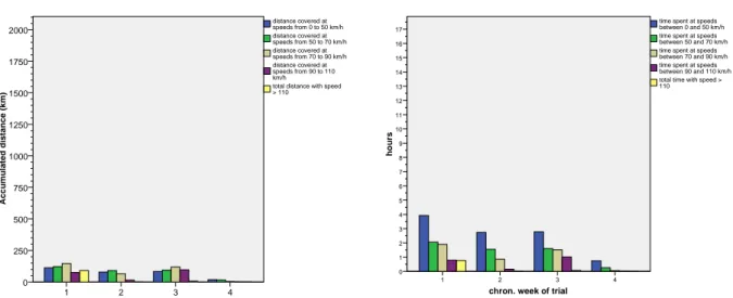
Participant 10 drove altogether 3,033.5 km distributed across 310 trips, resulting in an average trip length of almost 10 km. In fact, however, she took many very short in-town trips of below 3 km, and several longer trips, most of them 20 km in length, between work and home. In total she drove on 31 days, which results in almost 100 km per day on average. How the number of trips and several other variables were distributed for this participant in both the baseline and the treatment phase on trips above and below a length of 3 km can be seen in Table 3.

In the same table it is also presented which percentage of the total distance was logged and which percentage was lost due to computer booting and rebooting. For slightly above 10 % of the total distance no data are available at all. For the short trips this percentage is much higher, because the booting phase of the computer lasted for about one minute when booting correctly, resulting in a higher percentage of the whole trip for the shorter trips than for the longer ones. Additionally, in some cases the computer did not boot correctly at the first trial, such that 5 min passed until the hard reset enforced a reboot. In this case, depending on speed, up to about 5 km passed before data were logged.

(19)

Table 3 Statistics about distances and number of trips for Participant 10. baseline distance logged (in km) distance not logged (in km) total distance (in km) percent not logged of total number of trips total 913.2 133.8 1,047.0 12.8 113 above 3 km 861.2 109.4 970.6 11.3 72 below 3 km 52 24.4 76.4 31.9 41 treatment distance logged (in km) distance not logged (in km) total distance (in km) percent not logged of total number of trips total 1,806.1 180.4 1,986.5 9.1 197 above 3 km 1,705.3 136.9 1,842.2 7.4 107 below 3 km 100.8 43.5 144.3 30.1 90

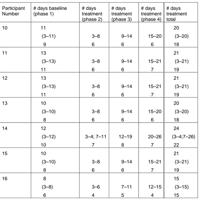
Figure 1 shows which distance respectively time the participant spent in different speed intervals. In Sweden the speed limit in urban areas is 50 km/h, on small rural roads it is 70 km/h, on larger rural roads it is 90 km/h, and on the motorway it is 110 km/h. The participant’s distribution across the different speed intervals in week four deviates from the other weeks to the effect that the participant drove faster than 110 km/h for a sub-stantial percentage of time during week 4, whereas she did not drive that fast at all during the other weeks. Speeds above 110 km/h are indicative of motorway driving, which differs from rural road driving in many ways. A closer analysis of the data showed that the participant took a trip of around 500 km round trip on the motorway during that week, whereas she did not use the motorway at all during the other three weeks.

The distribution across the different speed intervals is relatively similar in weeks 1 through 3. The interval [90 km/h; 110 km/h] is also overrepresented in week 4.

distance time 4 3 2 1 Acc u mul a ted di sta n ce (k m) 2000 1750 1500 1250 1000 750 500 250 0

total distance with speed > 110 distance covered at speeds from 90 to 110 km/h distance covered at speeds from 70 to 90 km/h distance covered at speeds from 50 to 70 km/h distance covered at speeds from 0 to 50 km/h 4 3 2 1 A ccum u la ted tim e (h) 17 16 15 14 13 12 11 10 9 8 7 6 5 4 3 2 1 0

total time with speed > 110 time spent at speeds between 90 and 110 km/h time spent at speeds between 70 and 90 km/h time spent at speeds between 50 and 70 km/h time spent at speeds between 0 and 50 km/h

Figure 1 Distribution of speed per distance and per time for the baseline phase and three separate phases during treatment.

(20)

3.2 Participant

11

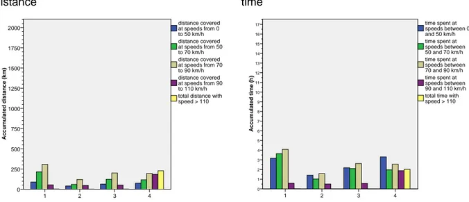
Participant 11 drove altogether 5,437.1 km distributed across 172 trips, resulting in an average trip length of 31.6 km. In total he drove on 34 days, which results in 160 km per day on average. During the baseline phase the average trip length was much longer than during the treatment phase. How the number of trips and several other variables were distributed for this participant in both the baseline and the treatment phase on trips above and below a length of 3 km can be seen in Table 4.

Table 4 Statistics about distances and number of trips for Participant 11.

baseline distance logged (in km) distance not logged (in km) total distance (in km) percent not logged of total number of trips total 3,095.6 42.8 3,138.4 1.3638 64 above 3 km 3,081.9 40.2 3,122.1 1.2876 51 below 3 km 13.7 2.6 16.3 15.9509 13 treatment distance logged (in km) distance not logged (in km) total distance (in km) percent not logged of total number of trips total 2,146.4 152.3 2,298.7 6.6255 108 above 3 km 2,116.1 140.6 2,256.7 6.2303 81 below 3 km 30.3 11.7 42 27.8571 27

This participant drove much more during week 1 than during the other three weeks, and he spent the major part of his driving during this week at speeds above 110 km/h. This participant generally engaged in a substantial amount of motorway driving. During week 2 he drove comparatively little, and the interval [90 km/h; 110 km/h] is under-represented during that week as compared to weeks 3 and 4. Those two weeks are relatively similar in the distribution of speed (Figure 2).

(21)

total distance with speed > 110 distance covered at speeds from 90 to 110 km/h distance covered at speeds from 70 to 90 km/h distance covered at speeds from 50 to 70 km/h distance covered at speeds from 0 to 50 km/h 4 3 2 1 A c cum u la ted tim e (h) 17 16 15 14 13 12 11 10 9 8 7 6 5 4 3 2 1 0

3.3 Participant

12

Participant 12 drove altogether 1,541.8 km distributed across 118 trips, resulting in an average trip length of 13.1 km. In total he had the car for 37 days, which results in 41.7 km per day on average. The average trip length was approximately equal for both phases. How the number of trips and several other variables were distributed for this participant in both the baseline and the treatment phase on trips above and below a length of 3 km can be seen in Table 5.

The participant shared the car with his girlfriend, because they car-pooled to his work, from where she then continued to her workplace. The girlfriend drove approximately 225 km during the baseline phase and approximately 300 km during the treatment phase. Her trips were excluded from the data analysis.

On several occasions the particpant wore a headband or a cap and had the collar of his jacket turned up, which impaired eye tracking. When he wore a headband with

(22)

Table 5 Statistics about distances and number of trips for Participant 12. baseline (both drivers) distance logged (in km) distance not logged (in km) total distance (in km) percent not logged of total number of trips total 847.9 85.9 933.8 9.199 75 above 3 km 825.2 79 904.2 8.737 59 below 3 km 22.7 6.9 29.6 23.3108 16 baseline (only intended driver) distance logged (in km) distance not logged (in km) total distance (in km) percent not logged of total number of trips total 654.3 54.1 708.4 7.6370 50 above 3 km 640.2 49.4 689.6 7.1636 39 below 3 km 14.1 4.7 18.8 25 11 treatment (both drivers) distance logged (in km) distance not logged (in km) total distance (in km) percent not logged of total number of trips total 993.4 146.6 1,140 12.8596 92 above 3 km 976.7 126.3 1,103 11.4506 73 below 3 km 16.7 20.3 37 54.8649 19 treatment (only intended driver) distance logged (in km) distance not logged (in km) total distance (in km) percent not logged of total number of trips total 734.2 99.2 833.4 11.9030 68 above 3 km total 726 89.9 815.9 11.0185 58 below 3 km total 8.2 9.3 17.5 53.1429 10

Compared to the other participants this participant drove very little. He spent about half of his driving time at speeds below 50 km/h and drove a lot in urban areas. The distri-bution across the different speed intervals is fairly equal for all four weeks (Figure 3).

(23)

3.4 Participant

13

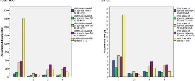
Participant 13 drove altogether 6,586.6 km distributed across 279 trips, resulting in an average trip length of 23.6 km. In total he drove on 30 days, which results in 220 km per day on average. During the baseline phase the average trip length was about 4 km longer than during the treatment phase. How the number of trips and several other variables were distributed for this participant in both the baseline and the treatment phase on trips above and below a length of 3 km can be seen in Table 6.

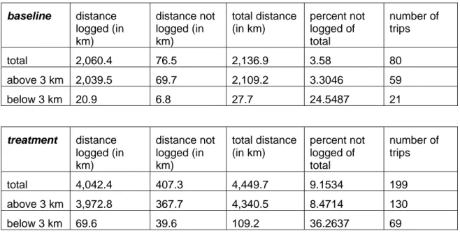
baseline distance logged (in km) distance not logged (in km) total distance (in km) percent not logged of total number of trips total 2,060.4 76.5 2,136.9 3.58 80 above 3 km 2,039.5 69.7 2,109.2 3.3046 59 below 3 km 20.9 6.8 27.7 24.5487 21 treatment distance logged (in km) distance not logged (in km) total distance (in km) percent not logged of total number of trips total 4,042.4 407.3 4,449.7 9.1534 199 above 3 km 3,972.8 367.7 4,340.5 8.4714 130 below 3 km 69.6 39.6 109.2 36.2637 69

(24)

This participant drove a lot on motorways during all four weeks. The distribution across the different intervals is fairly equal across the four weeks except for week 1, where the interval [0 km/h; 50 km/h] is slightly overrepresented.

distance time 4 3 2 1 A c cu m u lat e d d is tan c e (km ) 2000 1750 1500 1250 1000 750 500 250 0

3.5 Participant

14

Participant 14 drove altogether 7,407.5 km distributed across 368 logged trips. During one longer trip in the fourth week the data acquisition system was unstable and restarted after about five minutes for the whole duration of the trip. This resulted in a number of short trips in the log, instead of one long trip, which inflated the trip number somewhat, also in Table 7.

During the treatment phase, the sponsor of the project scheduled a demo event for stakeholders and the press and required the car to be on site. Therefore the treatment phase for this participant was interrupted on day 4 in the evening, when the car was picked up from the participant. It was returned to him on day 6 in the evening. Due to this the first week of the treatment phase was extended with two days (see Table 2). For this participant the eye tracking did not work as well as for the other participants. In many instances gaze tracking was lost and only head tracking was available. The video logs showed that the driver had a tendency of leaning his head back on the head rest, therefore he often “squinted” at the road with relatively closed eyes, which made it hard for the eye tracker to detect glance direction. Furthermore, the participant very often touched his face with his hand, thus, obstructing parts of the face from the view of the cameras.

(25)

Table 7 Statistics about distances and number of trips for Participant 14. baseline distance logged (in km) distance not logged (in km) total distance (in km) percent not logged of total number of trips total 4,172.8 117.3 4,290.1 2.7342 108 above 3 km 4,143 107.8 4,250.8 2.536 80 below 3 km 29.8 9.5 39.3 24.173 28 treatment distance logged (in km) distance not logged (in km) total distance (in km) percent not logged of total number of trips total 2,620.8 496.6 3,117.4 15.9299 260 above 3 km 2,540.7 449 2,989.7 15.0182 180 below 3 km 80.1 47.6 127.7 37.2749 80

This participant drove to Germany during the baseline phase, which is one reason for the much higher percentage of speeds above 110 km/h during the baseline phase than during the treatment phase. This trip explains, too, why the mileage during the baseline phase is that much higher than during the treatment phase (Figure 5).

total distance with speed > 110 distance covered at speeds from 90 to 110 km/h distance covered at speeds from 70 to 90 km/h distance covered at speeds from 50 to 70 km/h distance covered at speeds from 0 to 50 km/h

chron. week of trial 4 3 2 1 ho urs 17 16 15 14 13 12 11 10 9 8 7 6 5 4 3 2 1 0

3.6 Participant

15

Participant 15 drove 2,568.4 km altogether with the experimental car. Due to the fact that the log system had become unstable, it was not possible without manual post-processing to determine how many trips were driven. The number of trips in Table 8 is therefore misleading, too. It becomes apparent that the data loss increased from the baseline phase to the treatment phase, which indicates that the computer became

(26)

increasingly unstable over time. For the treatment phase one third of the distance was not logged, and in many instances the log was not only lost in the beginning of the trip, but also in the middle.

baseline distance logged (in km) distance not logged (in km) total distance (in km) percent not logged of total number of trips total 740.3 149.2 889.5 16.7735 80 above 3 km 709.1 133.9 843 15.8837 56 below 3 km 31.2 15.3 46.5 32.9032 24 treatment distance logged (in km) distance not logged (in km) total distance (in km) percent not logged of total number of trips total 1,101.5 577.4 1,678.9 34.3916 251 above 3 km 999.9 496.7 1,496.6 33.1886 149 below 3 km 101.6 80.7 182.3 44.2677 102

The speed distributions are relatively similar for the different phases and weeks. In all cases the participant drove below 50 km/h for a substantial part of the time and distance driven. In week 4 she drove relatively little, but during this week most data were lost, too. Speeds above 110 km/h occurred almost only during the baseline phase (Figure 6).

distance time 4 3 2 1 A c cu m u lat e d d is tan c e (km ) 2000 1750 1500 1250 1000 750 500 250 0

(27)

3.7 Participant

16

The car was returned to Saab for check-up due to the instability of the computer. Attempts were made to repair it, and it was decided to run Participant 16 as planned. Due to the approaching holidays and project end it was not possible to run a thorough trial to see whether the repairs had taken care of the computer crashes before the vehicle was handed over to the participant. It turned out that the problem had subsided

somewhat during the baseline phase, but reappeared during the treatment phase. Participant 16 drove 3,878.4 km in total, but for the same reasons as for Participant 15, namely the frequent computer crashes, it was not possible to determine how many trips she had made. During baseline driving data loss was limited to 6.6% of the total

distance, but during the treatment phase about a third of the data were lost (Table 9).

baseline distance logged (in km) distance not logged (in km) total distance (in km) percent not logged of total number of trips total 662.7 47.1 709.8 6.6357 47 above 3 km 652.1 45.2 697.3 6.4821 39 below 3 km 10.6 1.9 12.5 15.2 8 treatment distance logged (in km) distance not logged (in km) total distance (in km) percent not logged of total number of trips total 2,189.6 979 3,168.6 30.8969 143 above 3 km 2,150 957.1 3,107.1 30.8036 98 below 3 km 39.6 21.9 61.5 35.6098 45

The participant reported that she spent most of the time on the motorway, which is corroborated by the high percentage of speeds above 110 km/h. The speed distribution does not vary much across weeks, except that the percentage of speeds above 110 km/h is lower in the baseline phase than in the remaining weeks (Figure 7).

(28)

3.8 Comparison between participants

Mileage varied substantially between drivers, with Participant 12 having the smallest mileage and Participant 14 having driven almost five times as far within the same period of time (Table 10). Some participants drove the same route very often, because they mostly used the car for going to their workplace and back, while others drove many different routes. Three participants rarely drove above 110 km/h at all, whereas the other four spent a substantial part of their driving time at high speeds. Some parti-cipants showed relatively similar patterns across the four weeks of driving, while others had both very different mileages and different speed distribution patterns over the weeks.

Data loss was somewhat higher if the drivers took many small trips as compared to several longer ones. From the treatment phase of Participant 14 onwards it can be seen that data loss increased, then it fell again after the repairs before Participant 16 started, only to increase to a very high level again for the same participant’s treatment phase.

Table 10 Overview over mileage and percent data loss for baseline and treatment phase for all participants.

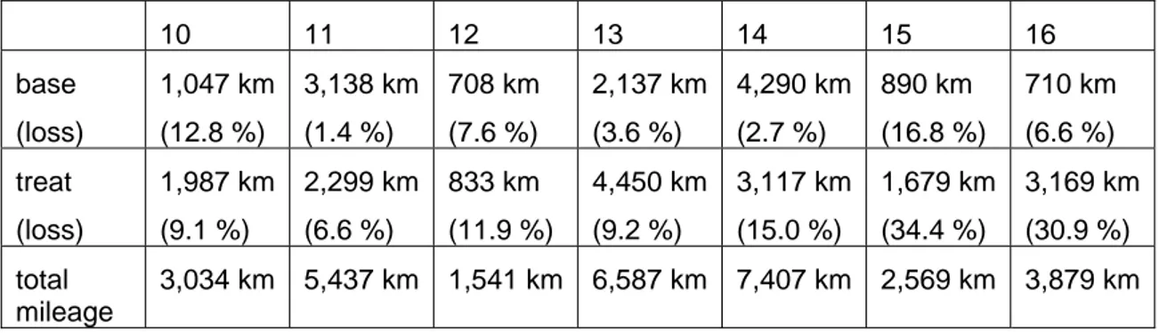
10 11 12 13 14 15 16 base (loss) 1,047 km (12.8 %) 3,138 km (1.4 %) 708 km (7.6 %) 2,137 km (3.6 %) 4,290 km (2.7 %) 890 km (16.8 %) 710 km (6.6 %) treat (loss) 1,987 km (9.1 %) 2,299 km (6.6 %) 833 km (11.9 %) 4,450 km (9.2 %) 3,117 km (15.0 %) 1,679 km (34.4 %) 3,169 km (30.9 %) total mileage 3,034 km 5,437 km 1,541 km 6,587 km 7,407 km 2,569 km 3,879 km

(29)

3.9 Discussion of trip statistics

The driving patterns of the participants varied both between and within participants, in the latter case between different weeks. Obviously, these different driving patterns reflect that drivers in the general population actually are very different from each other. This strong variation, together with the limited number of participants, complicates analysis and might cast doubts on some conclusions. For the most part the analyses will be made within subjects, but still considering the variation across subjects.

During field tests like this one, resembling FOTs with a relatively short driving time, special occurrences in driving patterns can have a relatively strong impact on the results. In this study one of the participants drove from Sweden to Germany and back in the baseline phase, which both led to a very high mileage during the baseline phase as compared to the treatment phase, and, more importantly, had some influence on the speed distribution during his driving. During the time when the study was conducted, the Swedish speed limits were 50 km/h, 70 km/h, 90 km/h and 110 km/h practically without exception. In Germany however, the speed limits are based on “even numbers”, and in some cases on the motorway there is no speed limit at all. Generally the driving environment is quite different in those two countries.

Another participant drove to Stockholm and back to Linköping, a total distance of about 400 km, during the third treatment phase, and it was only on that occasion that she used the motorway. During the other three weeks she only drove on country roads and urban roads. Therefore the speed distribution as well as the driving environment was consider-ably different between this part of the treatment phase and the remaining time.

The other participants did not exhibit too varying patterns during the time they had the experimental vehicle, but this factor definitely has to be considered in future studies. Both a larger number of participants and longer driving times can help reducing impacts of that kind. Other possibilities are to control the driving environment better, or to classify road types and analyse data from different road types separately. This would, however, probably also require a larger number of participants to guarantee enough relevant events on each road type.

In the present study the participants were run serially, because only one passenger car was available. This was done in a country with marked seasonal variations, both when it comes to weather and hours of daylight. Driving in summer with very long daylight hours and in most cases good road friction differs a lot from driving during the winter months, when it is dark for the most part of the day, and when road conditions can be of varying friction. On some road types the winter maintenance includes ploughing and salting, whereas other roads can be covered with packed snow. Icy roads can occur on a regular basis during winter. Thus, the participants in the present study dealt with very different environmental conditions, which definitely varied between participants, but which also varied within participants. The winter during which the data were logged was relatively mild with only little snow, which was advantageous from the point of view of the study.

However, in general in Sweden it is not unlikely that during one week the weather is mostly sunny, while it rains a lot during the next week. This could influence the parti-cipant’s behaviour more than the investigated safety system and should ideally be taken into account, either through logging and controlling for weather in the analyses, or by running enough participants in such a design that will most likely equal out possible confounding weather factors.

(30)

Generally, if unplanned influences like weather, type of road or hours of daylight cannot be randomised by a large enough number of participants and driving time, it would aid the interpretation of the results if matching situations could be found for analysis. One possibility would be to try to find a road segment that was frequented by all participants at least a certain number of times. If this proves impossible, a certain class of road might be used as selection criterion, possibly in combination with certain weather con-ditions. Any such special selection involves a substantial amount of more or less manual analysis, however, which did not fit into the budget frame of the present project. There-fore the only matching that was done for part of the analyses in this project was speed based. For some computations the results were split according to speed intervals that spanned 20 km/h. Often the speed interval of 0 to 50 km/h was excluded, because no warnings were given below 50 km/h, and all speeds above 110 km/h were subsumed into the same group. This was done to restrain the environmental variation within each group to some extent. Speeds of 110 km/h and above would occur mostly on motor-ways, speeds between 90 km/h and 110 km/h are very typical for relatively straight and well-built rural roads that can cover rather long distances. Speeds between 70 km/h and 90 km/h can often be found on smaller and more curvy rural roads, as well as on slight-ly more demanding sections on the bigger country roads, for example in junctions. Speeds between 50 km/h and 70 km/h are typical for suburban arterial roads and curvy and small rural roads. This classification takes into consideration that drivers often keep speeds that lie slightly above the posted speed limit. No cross-checking with the actual environment via GPS trace was conducted for the present analyses. The data are avail-able, however, and could probably be matched to the Swedish national road database, which would not only provide information on the road type, but also on speed limits, number of lanes, road signs and a host of other variables. Obviously, in built-up areas the GPS log has to be quite accurate in order to achieve a correct match.

With respect to the analysis of the number of trips, it would have been recommendable to analyse the time and the distance that passed between the end of one log file and the beginning of the next. This would have aided in determining actual trip length. This was not done, because there is no readily available information on how long a break between two “driving sessions” may be in order to consider two data files to belong to the same trip. It might also be the case that additional information like a new goal should be con-sidered when determining which unit is a trip. Thus, for simplicity reasons, and because this was not the focus of the study, it was decided to use a simple and easily applicable criterion for trip duration. Due to the computer crashes, however, not all files started with turning on the ignition and ended with turning it off.

(31)

4 Distraction

warnings

The data were pre-processed in the following way before the effect of the warning system on warning frequency was analysed: All trips taken during the first two days with the car were excluded, because it was assumed that the participants needed that time to get used to the car. The trips during the first two days with the system activated were excluded, too, due to the participants’ get used to the system. Additionally, all trips whose logs were shorter than 3 km were excluded, because during many of those short trips the participants rarely exceeded 50 km/h, the limit at which the distraction system began to work, and because those short logs were considered to be too idiosyn-cratic for a meaningful analysis. Finally, all trips during which the glance direction quality while driving did not exceed zero were excluded, because this indicated heavy problems with the eye tracking. This phenomenon occurred very rarely in general, and most often during very short trips.

In this chapter the frequency of distraction occurrences over time in general and in rela-tion to different speed intervals is discussed.

Distraction occurrences are those events for which the algorithm determines that the driver’s attention buffer is empty. Three different types of warnings were registered, which are direct warnings, inhibited warnings and indirect warnings.

Direct warnings are those that are issued to the driver immediately when the attention

buffer becomes empty. The driver is considered to be distracted.

Inhibited warnings are occasions during which the attention buffer is empty, but no

warning is issued either due to a speed below 50 km/h, activated direction indicators, the driver’s braking or moving the steering wheel a lot, the last warning having been initiated less than 15 seconds ago or due to other inhibiting factors (Kircher, K., Kircher, A. & Claezon, F., 2009).

Indirect warnings occur when a filter for inhibition is active at the time when the

atten-tion buffer is emptied, but the filter for inhibiatten-tion is deactivated while the attenatten-tion buffer still is empty. Then the warning is issued immediately when the filter is deacti-vated.

During the baseline phase the same rules applied. In order to prevent the warnings from reaching the driver, the plug that connected the seat vibrator to power was pulled. This physical measure is not considered to be an inhibiting factor as defined above, because it does not have anything to do with the algorithm, but only with the experimental design.

The duration since the last warning was computed in a way that for each warning it was determined how many seconds had passed since the last warning had been given. Each warning was treated as one case, regardless of its chronological position within one trip. The first warning in each trip was excluded, because no meaningful time since the last warning could be computed. The warnings were always sorted into the speed interval at which the warning occurred.

For the analyses presented below only direct warnings were considered. The reason for this is that preliminary data analyses showed that the indirect warnings often should have been inhibited as well, especially when they occurred directly after the inhibition ceased due to vehicle data, like speed increasing to above 50 km/h or the driver’s letting go of the brake. This is clarified with the help of an example:

(32)

When a driver leaves a roundabout, he often looks into the direction of the road he is going to drive onto, such that his gaze direction is not forward, but in the direction of the road he wants to continue on. In smaller roundabouts this direction may be located outside of the FRD. Often the speed in smaller roundabouts with stronger curves is below 50 km/h, though, therefore a warning for not looking at the FRD is inhibited. It happens, though, that the driver accelerates on his way out onto the other road, while still in the curve and still focusing his gaze into the direction of the remainder of the curve. If he exceeds 50 km/h during that phase, the speed inhibition is lifted. Then an indirect warning will be issued immediately if his attention buffer is still empty, even though the warning is not appropriate in this case. Analogous situations occur for braking. In the General Discussion under Section 11.6 ways to improve the AttenD algorithm are suggested, which also take this factor into consideration.

About one third of the indirect warnings occurred in the speed interval [50 km/h; 70 km/h], another third occurred at speeds above 110 km/h, and the remaining third occurred about equally distributed across the two intervals in the middle speed zones. Most of the direct warnings, which are computed by subtracting the number of indirect warnings from all warnings, are given at high speeds, whereas in the interval [50 km/h; 70 km/h] slightly fewer direct warnings are given than in the intervals in the middle speed zones (Table 11).

An analysis of the indirect warnings showed that in most of the cases they occurred about 15 s after the last issued warning, which indicates that they were given, because the inhibition that applied in the interval between [0 s; 15 s] after the start of the last warning was released, and the attention buffer was zero at the time. In the speed interval [50 km/h; 70 km/h] there was a tendency for longer intervals since the last warning was issued. This indicates that another main reason for indirect warnings in this speed interval was that the participants accelerated and exceeded 50 km/h while the attention buffer equalled zero. The number of indirect warnings was about 10% of all warnings for most of the participants. For Participant 12 the percentage of indirect warnings lay at 40%, and for Participant 14 the percentage lay at almost 30%, which is substantially higher than for the other participants. The actual number per participant and speed interval can be found in Table 11.

The average time that passed since a warning had been given is the content of this chapter. For the analyses the cases were split into the factors “week” and “speed cate-gory”. Week 1 represents the baseline, and week 2-4 represent the treatment condition. Exactly which days are included in which week can be found in Table 2. The warnings were sorted into different speed categories according to the speed at which the warning occurred. The speed at which the preceding warning was given was not considered. The boxplots presented below are vertical boxplots. The boundaries of the box are first and third quartile. The median is identified by the middle line in the box. The length of the box is the interquartile range (IQR). Values more than three IQR’s from the end of a box are labeled as extreme (*). Values more than 1.5 IQR’s but less than 3 IQR’s from the end of the box are labeled as outliers (O).

(33)

Table 11 The number of indirect distraction warnings and the total number of distraction warnings per participant and speed interval, including the “silent warnings” in the baseline phase.

Interval 10 11 12 13

indirect all indirect all indirect all indirect all

50–70 12 87 24 125 95 203 13 80 70–90 9 120 17 238 17 69 3 73 90–110 7 51 24 238 28 90 20 127 > 110 3 51 37 491 36 85 10 200 Total 31 309 102 1,092 176 447 46 480 Interval 14 15 16 Total (10-16)

indirect all indirect all indirect all indirect all

50-70 174 477 7 68 4 17 329 1,057 70-90 136 557 3 41 4 13 189 1,111 90-110 110 451 6 38 2 21 197 1,016 > 110 233 883 1 19 9 79 329 1,808 Total 653 2,368 17 166 19 130 1,044 4,992

4.1 Participant

10

A bug in the distraction detection software was found first after Participant 10 had completed her run. The bug affected 31 of the trips for this participant. They were spread approximately equally over the four weeks during which she had the car. Most of those trips were shorter than 3 km. All affected files were excluded from the data

analysis.

Table 12 Number of direct warnings given per week per speed category.

Interval 1 2 3 4 total 50–70 46 6 6 17 75 70–90 59 5 12 35 111 90–110 10 3 1 30 44 110+ 48 48 Total 115 14 19 130 278

Figure 8 shows the time in minutes that passed between warnings at different speeds per week with the experimental car. Table 12 indicates how many of those warnings were issued for each of the conditions, thus providing an estimate for the reliability of the mean.

(34)

chron. week of trial 4 3 2 1 8 7 6 5 4 3 2 1 0

Non-estimable means are not plotted chron. week of trial

4 3 2 1 ti m e si nce l ast warni ng (i n m in ) 15 10 5 0 110+ km/h 90 - 110 km/h 70 - 90 km/h 50 - 70 km/h Speed Categories

Figure 8 Estimated marginal means of the time in minutes since the last distraction warning was given per week per speed category (left) and boxplot of the time in minutes since the last distraction warning per week per speed category (right). Some extreme outliers are cut off for readability.

During the baseline week and during week 4 the participant drove substantially more and received many more warnings than during the other weeks. It also shows for those two weeks that the warning frequency does not vary much across speed categories. In weeks 2 and 3 where the mileage was lower and fewer warnings were received, the average frequencies vary more across speed categories, but it is likely that this is a result of the small number of observations.

The boxplot in Figure 8 shows, too, that the interquartile range is larger for the two middle weeks, during which only a small number of warnings was given, therefore mean values as those in Figure 8 should be viewed with caution. An analysis of variance with the factors week and speed category did not show any significant differences (F(12, 265) = 1.18).

4.2 Participant

11

For this participant all data files could be used, because the bug that had corrupted some of the files for Participant 10 had been fixed. The mileage of this participant was quite high, as was the number of warnings that he received.

Table 13 Number of direct warnings given per week per speed category.

Interval 1 2 3 4 total 50–70 45 19 12 25 101 70–90 90 31 40 60 221 90–110 81 11 70 52 214 110+ 347 23 55 29 454 Total 563 84 177 166 990

(35)

This participant covered many miles, especially during the baseline phase. He received a substantial number of warnings in almost each of the phases and speed intervals, which makes the results relatively reliable.

chron. week of trial

4 3 2 1 g 8 7 6 5 4 3 2 1 0

chron. week of trial

4 3 2 1 ti m e si nce last warni ng (i n m in) 15 10 5 0 110+ km/h 90 - 110 km/h 70 - 90 km/h 50 - 70 km/h Speed Categories

Figure 9 Estimated marginal means of the time in minutes since the last distraction warning was given per week per speed category (left) and boxplot of the time in minutes since the last distraction warning per week per speed category (right). Some extreme outliers are cut off for readability.

The mean intervals between two warnings are relatively equal across the different speed categories and across the four weeks (Figure 9). It appears that the mean duration between warnings decreased from the baseline phase to the first week in the treatment phase before returning to approximately the original level. No significant effects of the two factors week and speed interval were found, however (F(15, 974) = 0.97). The boxplot shows that the interquartile range for the intervals between warnings was approximately equal across speed categories and weeks, with the median having a tendency of being closer to the 25th quartile (Figure 9). For almost all boxes there are a substantial number of outliers and extremes, indicating that the variation in the time between warnings is quite big.

4.3 Participant

12

This participant had a relatively low mileage. He spent most of his driving time at lower speeds, where he also received most distraction warnings. In general, the number of distraction warnings per phase per speed category is relatively low for this participant, which indicates that mean values and distributions do not need to be very reliable (Table 14).