Thesis for the Degree of Bachelor’s in Computer Science – 15.0 hp
Anomaly detection in Network data with unsupervised
learning methods
George Sarossy
gsy16001@student.mdh.se
Examiner:
Sasikumar Punnekkat
Mälardalen University, Västerås, Sweden
Supervisor: Miguel León Ortiz
Mälardalen University, Västerås, Sweden
2
Abstract
Anomaly detection has become a crucial part of the protection of information and integrity. Due to the increase of cyber threats the demand for anomaly detection has grown for companies. Anomaly detection on time series data aims to detect unexpected behavior on the system. Anomalies often occur online, and companies need to be able to protect themselves from these intrusions. Multiple machine learning algorithms have been used and researched to solve the problem with anomaly detection and it is ongoing research to find the most optimal algorithms. Therefore, this study investigates algorithms such as K-means, Mean Shift and DBSCAN algorithm could be a solution for the problem. The study also investigates if combining the algorithms will improve the result. The results that the study reveals that the combinations of the algorithms perform slightly worse than the individual algorithms regarding speed and accuracy to detect anomalies. The algorithms without combinations did perform well during this study, they have slight differences between each other, and the results show the DBSCAN algorithm has slightly better total detection compared to the other algorithms and has slower execution time. The conclusion for this study reveals that the Mean Shift algorithm had the fastest execution time and the DBSCAN algorithm had the highest accuracy. The study also reveals most of the combinations between the algorithms did not improve during the fusion. However, the DBSCAN + Mean Shift fusion did improve the accuracy, and the K-means + Mean Shift fusion did improve the execution time.
3
Table of Contents
Abstract ... 2
1.
Introduction ... 5
2.
Background ... 6
2.1. Anomaly Detection ... 62.1.1. The types of anomalies ... 6
2.1.2. How to detect anomalies ... 7
2.2. Machine Learning ... 8 2.2.1. Unsupervised Learning... 8 2.2.2. Clustering ... 8 2.2.3. Dimensionality Reduction ... 11
3.
Related Work ... 12
4.
Problem Formulation ... 14
4.1. Limitations ... 145.
Method ... 15
6.
Ethical and Societal Considerations ... 16
7.
Design and implementation ... 17
7.1. Data set ... 17 7.1.1. Validation ... 17 7.1.2. Cross Validation ... 17 7.2. Used Algorithms ... 17 7.2.1. K-means... 17 7.2.2. Mean Shift ... 18 7.2.3. DBSCAN ... 18
7.2.4. Algorithm Combinations (fusion) ... 19
7.3. Experimental settings ... 20
7.3.1. K-means... 20
7.3.2. Mean Shift ... 20
7.3.3. DBSCAN ... 20
8.
Results... 21
8.1. Results of the Algorithms ... 21
8.1.1. K-means... 21
8.1.2. Mean Shift ... 23
8.1.3. DBSCAN ... 25
8.2. Results of the fusion of the Algorithms ... 27
8.2.1. K-means + Mean Shift ... 27
8.2.2. DBSCAN + K-means ... 28
4
8.2.4. DBSCAN + K-means + Mean Shift ... 30
8.3. Comparison with the related studies ... 31
9.
Discussion ... 32
10.
Conclusion ... 33
11.
Future Work ... 34
5
1. Introduction
Today most of our devices are connected to the internet and we use them all the time both in our professional and personal lives [1]. With more information being available online and more devices being connected,
cybersecurity has become more crucial than ever before [2]. With this evolution, online threats have evolved and become far more advanced and complicated. This makes it harder for companies to protect their data. For companies that use these devices in their networks, anomaly detection has become a crucial part of their
protection [1]. Critical systems are always being targeted by different attacks and succeeding attacks could result in very bad consequences. Some areas that consist of critical systems are markets, security, Internet of Things (IoT) Devices, and Business Analysis [2] [3]. These systems work online and could be breached, and they hold sensitive information that could cause a loss of currency, customers, and damage their brands’ reputation. These systems exist everywhere online, and we need to be able to protect them. That’s why we need to use anomaly detection to be able to detect potential indicators for breaches before they occur and to be able to resolve these intrusions in real-time before the security is broken.
Anomaly detection on time series data aims to detect unexpected behavior on the system [4]. As mentioned, before companies must be able to detect and predict anomalies on their network before they occur [1][2]. Companies have the responsibility to protect their users from attacks that could jeopardize their anonymity and their livelihood. When the anomaly detection methods are accurate it will be able to provide help to avoid losses in revenue and maintain the reputation of a company. Without anomaly detection companies will lose more than just their data, the branding and the reputation can be at risk if the users or supporters of that company get targeted from external attacks [4]. Because of this most companies are already using some sort of anomaly detection, when an anomaly is detected, it will send alerts to the operators then they will be able to decide on how to handle the problem and how to stop it to reoccur [5]. To solve this problem companies have started to use machine learning algorithms to detect anomalies that occur on the network.
This work aims to improve the accuracy and speed to detect and predict anomalies on networks for companies to protect themselves. My task in this thesis is to try out different Unsupervised Learning Algorithms to see which algorithms have the best accuracy and speed and try to run them in parallel. The algorithms the study will research are K-means, Density Based Spatial Clustering of Application with Noise (DBSCAN), and Mean shift.
The paper is organized as follows: In Section 2, everything that is necessary will be presented to be able to understand the thesis. In Section 3, some of the related works in the field will be presented and discussed. In Section 4, the problem, and the research questions will be presented. In Section 5, the method of the research will be provided. In Section 6, the ethical consideration will be defined. In Section 7, the design and
implementation will be provided. In Section 8, the result and the result comparison with the related studies will be presented. In Section 9, the discussion, in Section 10, the conclusion of the study will be presented. In Section 11, the future work will be presented.
6
2. Background
In this section, all the necessary information is provided for the study, and it is organized as follows: In Section 2.1, anomaly detection is described. In Section 2.2, machine learning is described. In Section 2.3, dimensionality reduction is described.
2.1. Anomaly Detection
Anomaly detection involves finding patterns in data that do not follow the expected behavior [2]. The patterns that do not follow the expected behavior in data, are often referred to as anomalies but has also more reference and could also be called outliers, surprises, discordant or contaminants in different application domains. The most used terms for anomaly detection are anomalies and outliers. Anomaly detection has many areas of use, some important areas in which this is used, are [2]:
• Intrusion detection is used for cyber-security to be able to analyze traffic patterns in a network system because if an anomalous traffic pattern enters the network, this could indicate that a computer that has been hacked sends sensitive data towards an unauthorized destination.
• Fault detection is used in safety-critical systems to be able to make sure these systems do not lead to failure, because it could lead to unacceptable consequences.
• Fraud detection is used for health care, insurance, or credit cards and it’s used for protecting individuals from outside attacks on their personal information and economy.
• Military surveillance is used to be able to detect the activities of the enemy.
2.1.1. The types of anomalies
There are three different types of anomalies, point anomalies, contextual anomalies, and collective anomalies [2]. The anomaly types are different from each other, the point anomaly is considered the simplest form of anomaly, when a single anomaly is detected in the data it is considered as a point anomaly. The point anomaly has most of the focus in anomaly detection research.
The most found anomalies in time series data are contextual. Contextual anomalies are labeled when the data sample is different in a particular context from the rest of the data, the characteristics of the data will decide if the anomaly can be labeled as contextual and known as a conditional anomaly [2], where some traits should be met to be able to label it as a contextual anomaly. The labeling is influenced by the structure of the data, which follows two sets of rules:
• The first rule is labeled as contextual attributes and it involves the method to determine the
neighborhood for the specific data sample [2]. Where in the time series data the attributes that must be looked at are the time, and that will help to give the position of the specific instance on the entire sequence.
• Then the second rule is behavioral attributes, and it involves the method to be able to look at the characteristics that are different from the contextual attributes, which means instead of looking at the time of the time series data it will look at how it behaves [2].
Then we have collective anomalies. Collective anomalies have gotten the term from when the data are different from the collection of the related data samples [2]. The individual data sample is not necessarily a collective anomaly but when the samples are joined together as a collection, it could be called a collective anomaly. The collective anomalies only occur in data sets where the data instances are related. But the other two types of anomalies depend on different concepts and rules that are mentioned above in this section.
7
2.1.2. How to detect anomalies
There are different ways to detect anomalies, the method is chosen depending on the characteristics of the data set [31].
• Proximity-based methods, methods identify anomalies when looking at each different data point in the data structure and apply a distance metric between each data point to determine if the data points are considered normal or anomalous. Different algorithms use this approach but the most used and known algorithm is the Local Outlier Factor (LOF) [6]. This algorithm looks through the data and assigns an outlier score for each reading, and the outlier score is based on the density measurements around their k nearest neighbors. Data points with high outlier scores are anomalies, otherwise, they are labeled as normal data.
• Clustering-based method is considered a subset of proximity-based algorithms. The clustering-based algorithms are creating clusters using the input data, and when new data arrives, it calculates which cluster the new data points belong to and assigns them to the closest cluster [7]. Each cluster can then be associated with a class label, which will be the label assigned to all data points in that cluster. • Statistical methods have wide usage, but many are measured from sensor inputs, and these algorithms
use data that has already been assigned and evaluates new data points based on past assignments. If new data points are evaluated to be statistically incompatible with the data that has already been evaluated, then it is labeled as an anomaly [8]. These algorithms are flexible and could be applied with different methods. Either it classifies one point at a time (Single readings), or it could work with batches of data
(Window readings). The window approach is often better than the single regarding reducing the number
of false positives, that is when a value is incorrectly labeled as an anomaly [9]. The most used window algorithm is called low-high pass filter, which uses the average of past data points and labels anomalies based on the difference between it, and the average of the previous data.
• Probabilistic method, this method uses a probabilistic model, these models have two subcategories that can be used, and the categories are parametric or non-parametric [26]. These algorithms can find anomalies by calculating the probability distribution to a probabilistic model. Data points are then labeled as anomalies if the calculated probability falls below a defined threshold. Two probabilistic models that are commonly used are Bayesian Networks [11] or the Hidden Markov method [10]. • Prediction-based methods use old data that has already been calculated to train algorithms that use a
predictive model [28]. With a trained mathematical model, the algorithm can predict future data points, and if new data are far too different from the predicted one, it is labeled an anomaly.
8
2.2. Machine Learning
Machine Learning (ML) is a subcategory in AI [12]. When a computer improves the algorithm automatically through experience, normally through a specific training process. A Machine Learning algorithm can predict an outcome from a set of input data by using statistical analysis. The algorithm will analyze the input data, then output a class, which is a representation of what the algorithm predicts that the input data represents, or it can predict an action [12]. The algorithm makes use of an underlying mathematical model to learn and build its experience. This is done through training, where the algorithm makes changes to the mathematical model with the experience it gets from the training process.
2.2.1. Unsupervised Learning
Unsupervised Learning (UL) does not use any labels [13]. Instead, it tries to find patterns in the data on its own, without getting any feedback on whether the predictions are right or wrong. These algorithms often find common patterns in data and can sort similar data points into groups. UL can also be developed to build a representation of the input data, this can be used to be able to predict future inputs, decision making and to be able to communicate and redirect the input data towards another machine. With this, it is safe to say the UL can learn how to find patterns in data where the unstructured noise isn’t considered pure [25]. There are different types of UL and two of the simplest examples of UL are clustering and dimensionality reduction.
2.2.2. Clustering
Clustering is also known as an unsupervised classification and the core of this method is to find groups of data points in a multidimensional data set [15]. Clustering is a way to separate unlabeled data set into a natural hidden data structure, instead of trying to find the accurate characterization of the new data set that has been provided to this method [16]. The clustering method use rules to decide what clusters the different data points will be assigned to, and it is with some metric or distance function [17]. Clustering methods are some of the oldest methods in machine learning. There are multiple clustering methods, some of the methods that can be used for clustering are K-means, Density Based Spatial Clustering of Application with Noise, and Mean Shift.
2.2.2.1. K-means
K-means is the most used unsupervised learning algorithm when performing clustering [18]. The k-means clustering algorithm will find clusters of data in a data set and determine which cluster the different types of data belong to. It will determine clusters with the help of the characteristics of the data set. The different clusters are built using similarities and differences between the different examples in the data set. The way K-means operates will be presented below and follows the information in [17]:
1. It starts with a default value of k, and the k is the number of clusters to find in the data set.
2. Then it randomly initializes the k cluster centers also known as centroids as, k samples in training data, with duplicate avoidance.
3. The algorithm will then assign each of the training samples to one of the centroids based on a chosen distance metric. The most used distance metric for this algorithm is the Euclidean distance metric.
4. Once the classes are created, and when the centroids are assigned, they will be recalculated to a new centroid. The new position of each centroid will be equal to the mean value of all the examples assigned to them and will happen for each cluster.
5. The algorithm will repeat steps 2-4 until the centroids do not change in one iteration.
9
2.2.2.2. Density Based Spatial Clustering of Application with Noise (DBSCAN)
DBSCAN is an unsupervised clustering algorithm, this algorithm is best suited for large data sets with noise because it can identify clusters with help of size and shapes [19]. DBSCAN identifies clusters with a density of points, which means that we have a higher density of points inside clusters and a lower density outside of them. When the density of points is lower it indicates that there is a cluster of noise or a cluster of outliers instead of clusters with the data we need. The DBSCAN algorithm follows a path where a cluster is defined by having at least one point, called a core point that satisfies the condition of having a minimum of MinPts neighbors in the range of predefined epsilon around it. The neighbor points also include their neighbors in the cluster if they are in the range of their epsilon (same size as the core point) but do not require MinPts neighbors if the cluster already has a core point [20]. Then the shape of the neighborhood is determined by the chosen distance function for the points p and q. The definition behind the DBSCAN algorithm will be presented down below and will follow [20]:
Definition 1: The epsilon-neighborhood of points p, indicated by 𝑁𝑒𝑝𝑠𝑖𝑙𝑜𝑛(𝑝), the shape of the neighborhood is
determined by the choice of the distance function for two points p and q 𝑁𝑒𝑝𝑠𝑖𝑙𝑜𝑛(𝑝) = {𝑞 ∈ 𝐷 |𝑑𝑖𝑠𝑡(𝑝, 𝑞) ≤ 𝑒𝑝𝑠𝑖𝑙𝑜𝑛}
Definition 2: (Directly density-reachable (DR)) In the cluster there are two types of pointers, one that represents the border p and one that represents the core points q. The difference between these pointers is that the border points are less in the neighborhood but can still be a part of a cluster if it belongs in the
epsilon-neighborhood but are less than the core points and the border points make a hull around the core points.
1. 𝑝 ∈ 𝑁𝑒𝑝𝑠𝑖𝑙𝑜𝑛(𝑞)
We can also assign q to a core point, but the epsilon-neighborhood is required to contain MinPts (minimum number of points) and the value of the MinPts tends to have a lower number assigned than the
epsilon-neighborhood to meet the core point condition.
2. |𝑁𝑒𝑝𝑠𝑖𝑙𝑜𝑛(𝑞)| ≥ 𝑀𝑖𝑛𝑃𝑡𝑠
Figure 2.1: Core and border points. Figure is taken from [20]
Definition 3: (Density reachable (DR)) is when A point p is DR from a point q with respect to epsilon and
MinPts if there is a chain of points: 𝑝1… , 𝑝𝑛, 𝑝1= 𝑞, 𝑝𝑛= 𝑝 𝑠𝑢𝑐ℎ 𝑡ℎ𝑎𝑡 𝑝𝑖+1 is directly DR from 𝑝𝑖.
Definition 4: (Density-connected (DC)) is when A point p is DC from a point q with respect to epsilon and
MinPts if there is a point o such that both, p and q are DR from o with respect to epsilon and MinPts.
Figure 2.2: Density reachability and connectivity. Figure is taken from [20]
Definition 5: (Cluster) If a point p is in a cluster A, a point q is also in cluster A only if it is DR from point p with the respect to a distance and MinPts within that distance.
10
When two points p and q belong to the same cluster C is parallel to point p and q being DC with the respect to
epsilon and MinPts
2. ∀𝑝, 𝑞 ∈ 𝐶: 𝑝 𝑖𝑠 𝐷𝐶 𝑡𝑜 𝑞 𝑤𝑖𝑡ℎ 𝑟𝑒𝑠𝑝𝑒𝑐𝑡 𝑡𝑜 𝑒𝑝𝑠𝑖𝑙𝑜𝑛 𝑎𝑛𝑑 𝑀𝑖𝑛𝑃𝑡𝑠
Definition 6: (Noise) Where we let 𝐶1, … , 𝐶𝑘 be the cluster if the database D with respect to parameters 𝑒𝑝𝑠𝑖𝑙𝑜𝑛𝑖
and 𝑀𝑖𝑛𝑃𝑡𝑠𝑖, 𝑖 = 1, … , 𝑘. Then the noise will be defined as a set of points in the database D where the point doesn’t belong to any cluster 𝐶𝑖, 𝑖. 𝑒. 𝑛𝑜𝑖𝑠𝑒 = {𝑝 ∈ 𝐷|∀ 𝑖: 𝑝 ∉ 𝐶𝑖}
2.2.2.3. Mean shift
Mean shift is a kernel-based method, and the usage of this algorithm is wide which is why it is commonly used in many applications [21]. Kernel-based methods work with both supervised learning and unsupervised learning. Mean shift is a hill-climbing algorithm that uses a kernel to look for high-density regions within the search space [32]. It does this by first defining a set of centroids in the search space. Each iteration shifts each centroid towards the high-density regions by calculating the mean of the points within a predefined radius around them, resulting in a mean shift vector that points towards a higher density region. The kernel defines how the average will be calculated, and there are several different kernels to choose from and are defined in [21]. When we have given n data points then will be lying in the Euclidean space which represents the kernel density estimation [22]. This can be explained mathematically and will follow [22]:
1. 𝑓𝑘(𝑥) = 𝐶𝑘,ℎ 𝑛 ∑ 𝑘 𝑛 𝑖=1 (||𝑥 − 𝑥𝑖|| 2 ℎ2 )
This will be based on a profile function k where a profile function is a normal graph that has the test values of the profiles saved.
2. 𝑘(𝑧) > 0 𝑧 ≥ 0
To ensure f will integrate to 1 the constant 𝐶𝑘,ℎ is chosen, where h is the bandwidth parameter which represents the radius. Which shows the maximum distance between the centroids and the data points. That will give a nonparametric estimator of the density at point x. Then this math formula could be further evolved to define 𝑔(𝑥) = −𝑘′(𝑥) with taking the gradient of (1.):
3. 𝑚ℎ(𝑥) = 𝐶∇𝑓𝑘(𝑥) 𝑓𝑔(𝑥) = ∑ 𝑥𝑖𝑔 (||𝑥 − 𝑥𝑖||2 ℎ2 ) 𝑛 𝑖=1 ∑𝑛 𝑔 𝑖=1 ( ||𝑥 − 𝑥𝑖||2 ℎ2 ) − 𝑥
The variable C in this instance is a positive constant and 𝑚ℎ(𝑥) is the mean shift vector. The function (3.) determines wheter the 𝑚ℎ(𝑥) is proportional to the density gradient estimate while normalized. With the
iteration 6. 𝑥(𝑗+1)= 𝑚
ℎ(𝑥(𝑗)) + 𝑥(𝑗) where points can be detected a rearranged to obtain the modes the
11
2.2.3. Dimensionality Reduction
Dimensionality reduction is important and used for transforming data that are represented in high dimensions into a reduced state of dimensionality, for the task to have a meaningful representation of the original data [23]. The field dimensionality reduction is important in are, signal processing, speech recognition, bioinformatics, and
neuroinformatic [23]. Working in a high dimensionality could be unpleasant because it could result in a curse of dimensionality. The curse of dimensionality increases the volume of space too fast and result in data becoming
sparse.
2.2.3.1. Principal Component Analysis (PCA)
The principal component analysis is a technique for dimensionality reduction, where PCA creates uncorrelated variables that will maximize the variance and minimize the information loss from the dimensionality reduction [24]. The uncorrelated variables will be found with the PCA algorithm, the algorithm needs to solve an
eigenvector problem to be able to find the variables. This happens with the help of the data set, and this results in an adaptive data analysis method. The PCA will reduce the dimensionality of the high-dimensional data set by embedding the data set into a linear subset with lower dimensionality [23]. The PCA could also be explained mathematically and will follow the explanation in [23]. The technique searches the matrix and tries to find a linear mapping (M) which is trying to maximize the cost function trace and with a mathematical representation of (𝑀𝑇 𝑐𝑜𝑣(𝑋)𝑀) where 𝑐𝑜𝑣 is the sample covariance matrix and (𝑋) is the data set that is used. Then the linear
mapping is created with the d principal eigenvectors also known as principal components of the sample covariance matrix, where the mean data is zero [23]. With this, the eigenproblem is solved with this equation: 𝑐𝑜𝑣(𝑋)𝑀 = 𝜆𝑀 [23]. The eigenproblem is solved for d principal eigenvalues 𝜆. The representation of the low dimensional data set labeled as 𝑦𝑖 of the data points 𝑥𝑖 and will be calculated when mapping the representation at the linear basis 𝑀, 𝑖. 𝑒. , 𝑌 = 𝑋𝑀. This technique uses Euclidean distance 𝑑𝑖𝑗 for calculating the distances between data points in high and low dimensionality, where 𝑥𝑖 𝑎𝑛𝑑 𝑥𝑗 represent the high-dimensional space. To be able to use the classical scaling method the technique finds the linear mapping where the Euclidean distance could be applied on: ∅(𝑌) = ∑ (𝑑𝑖𝑗2 − ||𝑦
𝑖− 𝑦𝑗||2)
𝑖𝑗 in which ||𝑦𝑖− 𝑦𝑗||2 represents the squared Euclidean
12
3. Related Work
In [27], M. A. Kabir and X. Lou investigate and evaluate different unsupervised learning algorithms to see which of them has the better detection rate and lowest false-positive rate. The algorithms they are testing are K-Means, Self-organizing Maps (SOM), deep autoencoding Gaussian mixture model (DAGMM), and adversarially learned anomaly detection (ALAD). They set two different benchmark data sets for the network flow-based anomaly detection, while they test different parameters and neural network settings for each UL algorithm. The results they found during their work was that the DAGMM algorithm gains the lowest false-positive rate and a high result for anomaly detection rate, it worked better on one of the data sets compared to the other. Where the SOM algorithm gained the best result on the other data set. When they compared the anomaly detection rate for each algorithm, they found out that K-means works better than the other algorithms when the unseen attacks have no instances in the training set. When the attacks have a few instances on the training set, the algorithm ALAD worked better because it uses an adversarial sample generation mechanism. They concluded that the algorithms they used had stable performances and were easy to implement, and the ALAD algorithm showed excellent results in the detection of minority attacks. Then they also concluded that to be able to achieve better results they should integrate the algorithms for network flow anomaly detection.
In [28], E. Swartling, and P. Hanna, investigated DBSCAN and the LOF algorithms for identifying anomalies on unlabeled data, they focused on the damage identification for industries in their production process. They observed the pump-generated data during execution, and used high frequency sampled current and voltage time series data for identification. The collected data was split up into five different phases, the startup phase, three duty point phases, and the shutdown phase. They concluded that the DBSCAN and LOF algorithm identifies unexpected data points within their data set, and they state that their problem was around the validation of the points. Their validation method had two parts to it, first, they needed to investigate if the data point that has been found was an outlier or not compared to the rest of the data in the set, the second part to the validation was if the outliers were indeed an anomalous behavior. Their study resulted in that they found out when increasing the number of dimensions then the number of outliers will increase rapidly for both DBSCAN and LOF. With this result, they stated that the algorithms are less confident when the outlier number increases, because the graph curve is getting flatter, and is visible for the duty points. They concluded the methods they used could identify unexpected data points within their set.
In [29], B. Georgescu, I. Shimshoni, and P. Meer investigate how to reduce the computational complexity of adaptive mean shift. They have investigated the most popular techniques for clustering and listed what kind of limitations they hold. The first clustering method they investigated was the k-means algorithm and they have stated the limitation the technique beholds. The limitation they have mentioned is, k-means need to know the number of clusters before execution, and the clusters are constrained to be spherically symmetric. The second method they investigated was nonparametric clustering methods that are based on mean shift, and they state that the limitations of this method will be eliminated, and when the dimension of space increases then the amount of computation becomes prohibitively large. They want to find a way to reduce the computation complexity and during the time of the report, there was a recently proposed approximation technique that could help with the reduction of the computation complexity. The method they used was locality-sensitive hashing (LSH), but they have changed the implementation of the method and states that with their way of implementing the method they find the optimal parameters of the data structure and will be determined by a pilot learning procedure, with the help of data-driven partitions. Their conclusion to this study was that with the help of a data structure that was based on a locality-sensitive hashing method they obtained a significant decrease in the run time and at the same time they maintained the quality of the result. The results they got during this study for k-means and the adaptive mean shift algorithm was that the k-means algorithm could classify 97.32% and the adaptive mean shift (AMS) could classify 98.66% for the Brodatz database.
13
In [30], the authors’ goal was to develop a time-series anomaly detection service for the customers at Microsoft, their goal was to achieve monitorization of the time-series in the time-series so the customers could be alert for incidents that could occur. In their paper, they are introducing the pipeline and the algorithms for their anomaly detection service, with the design for accuracy, efficiency, and to be general. Their pipeline structure is built upon three major modules, and includes data ingestion, online computing, and experimentation platform. To be able to handle the problem with anomaly detection on time-series they have proposed a novel algorithm that will be based on Convolutional Neural Network (CNN) and Spectral Residual (SR). They attempted to apply the SR model on time-series anomaly detection with a borrowed SR model from the visual saliency detection domain. They combined both models SR and CNN to improve the performance of the SR model, their statement on this combination is that their approach achieves superior experimental results compared with the state-of-the-art baselines towards Microsoft production data and public data sets. Their conclusion states that time-series anomaly detection is a critical module, that is because they need to ensure the online service quality. They also conclude that if the anomaly detection system is efficient, general, and accurate the system would be
14
4. Problem Formulation
The internet is used all the time [1], both in our private life and for work. Devices are connected to the internet where anomalies could occur. Both companies and people in private need to be able to protect themselves from intrusions. Anomaly detection has become a crucial part of the protection of information and integrity. With information being available online and more devices being connected, cybersecurity has become more crucial than ever before [2]. Because of this, I will choose different Unsupervised Machine Learning Algorithms to decide how we can detect and predict anomalies. In this study I will implement and compare unsupervised learning algorithms, to see whether I can find a good way to solve the anomaly detection problem efficiently.
The research questions are therefore defined as:
● Which Machine Learning Algorithm has the highest detection rate and speed? ● Can combining different algorithms give better results?
4.1. Limitations
The limitations I will encounter during this thesis are the depth of the data set and what algorithms I will be using. No data set includes every single possible anomaly that could occur for any company network.
15
5. Method
In this Section, the method of the work is provided.
This will be an empirical study. In the beginning, a literature study was conducted to find more information regarding which algorithms are good for anomaly detection, then choose the unsupervised learning algorithms and find more information about the chosen algorithms: K-means, Density Based Spatial Clustering of Application with Noise and Mean Shift and more information regarding Network Anomaly Detection and Principal Component Analysis (PCA). I will use the data set (KDD99) that included several different anomalies based on real data. The data set will be used to test the algorithms and how they perform. I will look through related studies around the algorithms I have chosen to see if they are performing similarly to my algorithms.
When I have chosen the algorithms, this study will become an experimental study, where each of the
unsupervised learning algorithms will be implemented and tested on the chosen data set. With the test data, I will compare the results of each algorithm against each other and the related studies. I will compare accuracy and speed to determine whether some of the algorithms are better suited than others for detecting anomalies in networks. I will then combine (fusion) all the algorithms with each other and the most accurate algorithm and the algorithm with the lowest execution time. Then observe if the result will be improved and whether this could be a workable solution to this kind of problem.
I will then pick the fastest algorithm, and the one with the highest accuracy, and test if running them simultaneously can improve the overall result, and whether this could be a feasible solution to this kind of problem.
To do this I need to investigate:
1. Which algorithms have the best performance regarding accuracy and speed for anomaly detection. 2. Test the algorithms towards a data set.
3. Record how many anomalies each algorithm could find and how fast.
4. Try to combine all the algorithms and the most accurate algorithm and the fastest algorithm and run them simultaneously to see if the result changes.
16
6. Ethical and Societal Considerations
I won’t be using any confidential data because the data set (KDD99) I will use is already publicly available for all to use.
17
7. Design and implementation
This Section will be organized as follows: Section 7.1 the data set is presented. In Section 7.2 the used algorithms will be presented. In Section 7.3 the experimental settings are presented.
7.1. Data set
The data set used in this study is KDD99 and has been used in competition more specifically The Third
International Knowledge Discovery and Data Mining Tools Competition [14]. The KDD99 data set was made to have a training set and a test set, each set contains a different amount of attack types [14]. The training set contains 22 specific attacks however the test set contains 37 attacks.
7.1.1. Validation
The labeling of the clusters started after each algorithm’s execution, and the algorithms have generated an array where each data point had been assigned a cluster. When the data points have been assigned to each cluster, the algorithms went through each data point and checked which of each type are most common in the cluster then assigned a label to the specific cluster. The clusters got divided into two different label groups, “normal”, “attack” cluster groups. Then the algorithm went through the KDD99 data set and checked each data point if the assigned group were correct or not with the original labels in the data set. The algorithm calculated if each data point wherein the correctly assigned cluster and gave out a percentage on accuracy for each algorithm.
7.1.2. Cross Validation
Each algorithm got executed ten times on the same data set, then I calculated the average accuracy for all the ten executions for each algorithm.
7.2. Used Algorithms
The algorithms are written in MATLAB language using the Statistics and Machine Learning Toolbox, and the used data set is KDD99 for each algorithm. The k-means algorithm is from the Statistics and Machine Learning Toolbox. The Mean Shift and DBSCAN algorithms were implemented without any toolbox.
7.2.1. K-means
The K-means algorithm I used during this study works as follows: declare the number of clusters prior to the execution, then loop through the number of clusters and initialize randomly centroids on the search space. For each sample in the data set X assign the closest centroid to each sample with the Euclidean distance metric. Then save all the centroids that has been added to a new variable, while centroids are not equal to the old centroids. Then update all the centroids on the sample s by calculating the mean value of all the assigned samples. Last step is to create a vector called idx which contains each data points assigned cluster index. Loop through each data point and check which cluster/centroid it belongs to. Then add that index to the idx vector.
The Algorithm 1 is the pseudocode for this.
Algorithm 1: K-means
Input: two parameters: k (number of clusters), X (Data set) Output: An array with each points assigned a cluster number
1. k = n
2. For i = to k do
3. centroids[i] initialize the centroids randomly on the search space 4. oldCentroids = NULL
5. While Centroids != oldCentroids do 6. For each s in X
7. s.Assign_the_centroids 8. oldCentroids = centroids
9. Centroids update_centroids on s 10. idx = {01, 02, 03 … 0𝑛}
18 12. for j = 1: numCentroids The number of centroids 13. if 𝑥𝑖 is in 𝑐𝑒𝑛𝑡𝑟𝑜𝑖𝑑𝑗 then
14. Idx[i] = j
7.2.2. Mean Shift
The Mean Shift algorithm I used during this study works as follows: First step is to loop through the number of centroids randomly initialized into the search space. For each centroid in centroids, then assigning samples within the radius to the centroid k, with the Euclidean Distance Metric. Save the centroids assigned to a new variable oldCentroids. Then calculate the mean value of all samples assigned. This is executed while centroids are not equal to old centroids. Last step is to create a vector called idx which contains each data points assigned cluster index. Loop through each data point and check which cluster/centroid it belongs to. Then add that index to the idx vector.
The Algorithm 2 is the pseudocode for this.
Algorithm 2: Mean shift
Input: three parameters: k (number of centroids), R radius (assigning points to each centroid), d (distance
between each centroid)
Output: An array with each points assigned a cluster number
1. For i = 1 to k do
2. centroids[i] //Will be initialized into the search space 3. oldCentroid = Null
4. While Centroids != oldCentroids do 5. For each centroid k in centroids 6. k.assign_the_samples 7. oldCentroids centroids
8. Centroids update the centroids by calculating the mean value for all samples 9. idx = {01, 02, 03 … 0𝑛}
10. for each datapoint 𝑥𝑖 in X
11. for j = 1: numCentroids The number of centroids 12. if 𝑥𝑖 is in 𝑐𝑒𝑛𝑡𝑟𝑜𝑖𝑑𝑗 then
13. Idx[i] = j
7.2.3. DBSCAN
The DBSCAN algorithm I used during this study works as follows: Declare the data set and the epsilon and minpts to the algorithm. Then for each unvisited points x in the data set, then mark x as visited. Then find the neighboring data points that are in range of the surrounding epsilon and add them to set N. if the size of N is less then minpts then mark x as noise. Else create cluster C for x, for each neighboring point x´ in N, find the neighbors again, and add those to N´. If neighbor of x´ is not visited, then mark neighbor as visited. If the size of the neighbors N´ is equal or higher then minpts, then combine N with the N´. If the x´is not member of any cluster then add x´ to cluster C. Last step is to create a vector called idx which contains each data points assigned cluster index. Loop through each data point and check which cluster/centroid it belongs to. Then add that index to the idx vector.
The Algorithm 3 is the pseudocode for this.
Algorithm 3: DBSCAN
Input: three parameters: the data set X, the distance threshold between points epsilon(eps) and minimum
number of points needed to be able to from a cluster, minpts
Output: An array with each points assigned a cluster number
1. DBSCAN(X, eps, minpts)
2. For each unvisited point 𝑥𝑖 in X do 3. mark x as visited
4. N get_neighbors(x,eps) 5. If size of N < minpts then
19 6. mark x as noise
7. else 8. C {x}
9. for each point x´ in N do 10. N N \ x´
11. if x´ is not visited then 12. mark x´ as visited
13. N´ get_neighbors(x´,eps) 14. if size of N´ ≥ minpts then 15. N N combine N´
16. if x´ is not yet member of any cluster then 17. C C combine {x´}
18. idx = {01, 02, 03 … 0𝑛}
19. for each datapoint 𝑥𝑖 in X
20. for j = 1: numCentroids The number of centroids 21. if 𝑥𝑖 is in 𝑐𝑒𝑛𝑡𝑟𝑜𝑖𝑑𝑗 then
22. Idx[i] = j
7.2.4. Algorithm Combinations (fusion)
The following combinations were created and used: • K-means + Mean Shift
• DBSCAN + K-means • DBSCAN + Mean Shift
• DBSCAN + K-means + Mean Shift
The combinations were created by training the algorithms in parallel, combining the centroids, and then calculating the Euclidean distance between new data points from the test data set and the combined centroids. I assign the cluster of the closest centroid to the data point.
20
7.3. Experimental settings
The settings for each algorithm are presented down below:
7.3.1. K-means
To find the optimal cluster size (202) I tried every cluster size from 1 to 500, in the validation set. The output of the execution showed the cluster size 202 is the most optimal for the data set.
K-means settings: X = data set (KDD99_10%), k = 202 (number of clusters).
7.3.2. Mean Shift
PCA is used during the Mean Shift execution to reduce the dimensions to two.
Mean Shift settings: X = data set (KDD99_10%), k = 100, R = 1, d = 1.6.
The process of finding the best parameters was done with a loop. The range I used during the loop was the R values between 1-2, increased with 0.1 for each iteration and the d values between 1-5, increased with 0.1 for each iteration.
7.3.3. DBSCAN
The process of finding the best parameters takes time with this algorithm. The massive amount of data points in the data set is the cause of the long execution time. The algorithm will look through every data point one by one and calculate the Euclidean distance for all of them. I ran the DBSCAN algorithm on a smaller data set to find a pattern on how the epsilon and MinPts values affected the accuracy of detecting normal clusters and anomaly clusters. Then I ran the DBSCAN algorithm on a larger data set to observe if the same pattern would occur. The range I used during this process was epsilon values between 1-150 and the MinPts values 1-200.
DBSCAN settings: X = data set (KDD99_10%), eps = 1, minpts = 1. (These points work well with smaller data sets but gives out of memory error with larger data sets.)
The KDD99_10% data set was used because of memory issues where the algorithm tried to save too many calculations at once in the ram.
21
8. Results
This section will be presented as follows: In Section 8.1, the result of each algorithm is presented. In Section 8.2 the result of the combined algorithms is presented. In Section 8.3 the comparison between the related studies is presented.
8.1. Results of the Algorithms
8.1.1. K-means
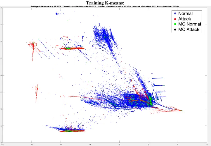
In Figure 8.1 we can see the following results: Average total accuracy: 98.87%, Correct classified normals: 99.83%, Correct classified attacks 97.90%, Number of clusters: 202, Execution time: 25.59s.
Training K-means:
Figure 8.1 Image of the created clusters provided by the K-means training execution. Where the blue color indicates the normal clusters, the red color indicates the attack clusters, the green color indicates the misclassified normal clusters, and the black color indicates the misclassified attack clusters. PCA is used for
22
In Figure 8.2 we can see the following results: Average total accuracy: 99.19%, Correct classified normals: 99.90%, Correct classified attacks 98.47%, Number of clusters: 202, Execution time: 15.67s.
Testing K-means:
Figure 8.2 Image of the created clusters provided by the K-means testing execution. Where the blue color indicates the normal clusters, the red color indicates the attack clusters, the green color indicates the misclassified normal clusters, and the black color indicates the misclassified attack clusters. PCA is used for
plotting in 2d.
The results of the K-means algorithm show that the testing phase provides a slightly better result. The Average total accuracy is higher in the testing case by 0.32% and the execution speed is 9,92 seconds faster than the training case.
23
8.1.2. Mean Shift
In Figure 8.3 we can see the following results: Average total accuracy: 98.64%, Correct classified normals: 98.74%, Correct classified attacks 98.54%, Number of clusters: 85, Execution time: 33.10s.
Training Mean Shift:
Figure 8.3 Image of the created clusters provided by the Mean Shift training execution. Where the blue color
indicates the normal clusters, the red color indicates the attack clusters, the green color indicates the misclassified normal clusters, and the black color indicates the misclassified attack clusters. PCA is used for
24
In Figure 8.3 we can see the following results: Average total accuracy: 99.17%, Correct classified normals: 98.84%, Correct classified attacks 99.50%, Number of clusters: 85, Execution time: 2.81s.
Testing Mean Shift:
Figure 8.4 Image of the created clusters provided by the Mean Shift testing execution. Where the blue color
indicates the normal clusters, the red color indicates the attack clusters, the green color indicates the misclassified normal clusters, and the black color indicates the misclassified attack clusters. PCA is used for
plotting in 2d.
The results of the Mean shift algorithm show that the testing phase provides a slightly better result. The Average total accuracy is higher in the testing case by 0.53% and the execution speed is 30,29 seconds faster than the training case.
25
8.1.3. DBSCAN
In Figure 8.5 we can see the following results: Average total accuracy: 100%, Correct classified normals: 100%, Correct classified attacks 100%, Number of clusters: 104480, Execution time: 4177.49s.
Training DBSCAN:
Figure 8.5 Image of the created clusters provided by the DBSCAN training execution. Where the blue color
indicates the normal clusters, the red color indicates the attack clusters, and the green color indicates the misclassified normal clusters. PCA is used for plotting in 2d.
26
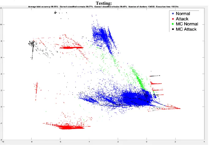
In Figure 8.6 we can see the following results: Average total accuracy: 99.87%, Correct classified normals: 99.84%, Correct classified attacks 99.90%, Number of clusters: 103299, Execution time: 765.96s.
Testing DBSCAN:
Figure 8.6 Image of the created clusters provided by the DBSCAN testing execution. Where the blue color
indicates the normal clusters, the red color indicates the attack clusters, the green color indicates the misclassified normal clusters, and the black color indicates the misclassified attack clusters. PCA is used for
plotting in 2d.
The results of the DBSCAN algorithm show that the training phase provides a slightly better result. The Average total accuracy is higher in the training case by 0.13% and the execution speed of the testing is 3411,53 seconds faster than the training case.
The testing results from each algorithm: Algorithm: Average total
accuracy in % Correct classified normal in % Correct classified attacks in % Number of clusters Time in seconds K-means 99.19 99.90 98.47 202 15.67 Mean Shift 99.17 98.84 99.50 85 2.81 DBSCAN 99.87 99.84 99.90 103299 765.96
The DBSCAN testing algorithm shows slightly better average total detected results compared to the other algorithms. The Mean Shift algorithm has a slightly faster execution time than the K-means algorithm and has a faster execution time than the DBSCAN algorithm. The Mean Shift algorithm also has a lower number of clusters compared to the other algorithms, with a slightly lower anomaly detection percentage than K-means and DBSCAN.
27
8.2. Results of the fusion of the Algorithms
8.2.1. K-means + Mean Shift
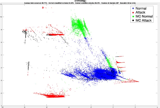
In Figure 8.7 we can see the following results: Average total accuracy: 96.77%, Correct classified normals: 94.10%, Correct classified attacks 99.45%, Number of clusters: 287, Execution time: 3.40s.
Testing:
Figure 8.7 Image of the created clusters provided by the K-means + Mean Shift testing execution. Where the
blue color indicates the normal clusters, the red color indicates the attack clusters, the green color indicates the misclassified normal clusters, and the black color indicates the misclassified attack clusters. PCA is used for
28
8.2.2. DBSCAN + K-means
In Figure 8.68 we can see the following results: Average total accuracy: 97.00%, Correct classified normals: 94.62%, Correct classified attacks 99.39%, Number of clusters: 103310, Execution time: 203.99s.
Test result:
Figure 8.8 Image of the created clusters provided by the DBSCAN + K-means testing execution. Where the blue
color indicates the normal clusters, the red color indicates the attack clusters, the green color indicates the misclassified normal clusters, and the black color indicates the misclassified attack clusters. PCA is used for
29
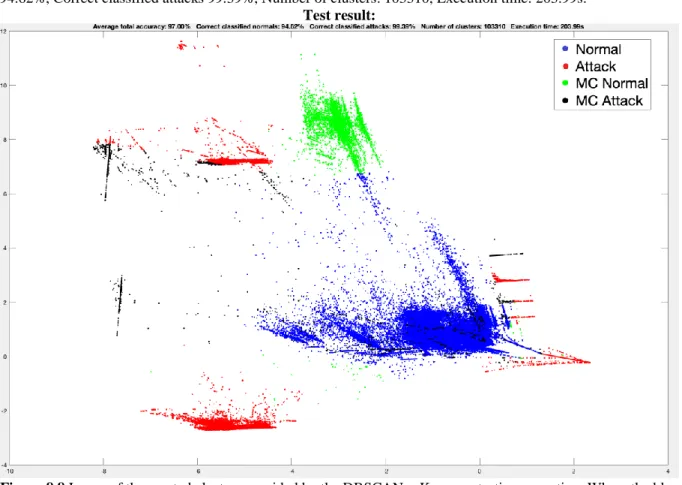
8.2.3. DBSCAN + Mean Shift
In Figure 8.9 we can see the following results: Average total accuracy: 99.25%, Correct classified normals: 99.07%, Correct classified attacks 99.42%, Number of clusters: 104565, Execution time: 192.81.
Testing:
Figure 8.9 Image of the created clusters provided by the DBSCAN + Mean Shift testing execution. Where the
blue color indicates the normal clusters, the red color indicates the attack clusters, the green color indicates the misclassified normal clusters, and the black color indicates the misclassified attack clusters. PCA is used for
30
8.2.4. DBSCAN + K-means + Mean Shift
In Figure 8.10 we can see the following results: Average total accuracy: 96.82%, Correct classified normals: 94.19%, Correct classified attacks 99.44%, Number of clusters: 104767, Execution time: 174.07s.
Testing:
Figure 8.10 Image of the created clusters provided by the DBSCAN + K-means + Mean Shift testing execution.
Where the blue color indicates the normal clusters, the red color indicates the attack clusters, the green color indicates the misclassified normal clusters, and the black color indicates the misclassified attack clusters. PCA is
used for plotting in 2d.
The results of the fusion: Algorithm: Average total
accuracy in % Correct classified normal in % Correct classified attacks in % Number of clusters Time in seconds K-means + Mean Shift Figure 8.7 96.77 94.10 99.45 287 3.40 DBSCAN + K-means Figure 8.8 97.00 94.62 99.39 103310 203.99 DBSCAN + Mean Shift Figure 8.9 99.25 99.07 99.42 104565 182.81 DBSCAN + K- Means + Mean Shift, Figure 8.10 96.82 94.19 99.44 104767 174.07
The results of the fusion between the algorithms performed worse than the algorithms without the fusion. The accuracy dropped for almost every algorithm except DBSCAN + Mean Shift which gives the highest average accuracy at 99.25%. The K-Means + Mean Shift fusion had the fastest time with 3.40s and the lowest number of clusters of 287. Then on second place was the DBSCAN + Mean Shift + K-means with 174.07s and with a cluster number of 104767.
31
8.3. Comparison with the related studies
Comparison of the results between the algorithms that used the KDD99 data set in the related studies and this study:
Algorithm: Average total accuracy in %
K-means 99.19
K-means [27] 99.8
Comparison between each result showed that the algorithm from the related study [27] had a better result in accuracy in total, with a lower number of clusters. The execution time was not presented in their study, a comparison between the execution times could not be done.
32
9. Discussion
In this Section, the result from the previous Section is discussed.
The results of the related study that uses the same data set [27] can be observed in Section 8.3 and give a higher percentage than the result in this study. Some factors can affect why the results are different, the first factor is the usage of data sets. The usage of the data set could be summarized as how they train and test their algorithm, and how they divided the testing and training. The results can also differ in the development of the algorithms. In [27] they did not present how they built their k-means algorithm and what distance metric they used. In [28] they used the same DBSCAN as I did but had a different data set for testing and training. In the study [29] they used Adaptive Mean Shift and K-means, and I used the normal Mean Shift for clustering. They also used a different data set for testing and training. That is why I could not use the results in [28][29] as a comparison for my work.
The fastest algorithm was the Mean Shift algorithm, and the most accurate algorithm was DBSCAN. The result of the Mean Shift algorithm was not expected because it had a slower execution time than K-means in training. The DBSCAN algorithm performed almost as expected, the algorithm had a slower execution time in both training and testing but had the highest accuracy in both cases compared to the other algorithms. It is because the algorithm checks every data point in the search space and calculates the Euclidean distance between each data point in the search space during multiple iterations. This method makes the algorithm go slower but can have a higher accuracy overall through the whole execution. The DBSCAN algorithm had a slower execution time in testing as mentioned above but improved itself with 3411,53s. That is because the algorithm is calculating the Euclidean distance between the important data points the algorithm has selected in training which results in far fewer calculations. The K-means algorithm did not perform as expected, because it had the fastest execution time compared to the other algorithms in training but got a slower execution time compared to Mean Shift in testing. The reason why the k-means algorithm was expected to have the fastest execution time is that how the algorithm works. The Euclidean distance is calculated between each centroid in the search space. This method provides a faster speed of execution because there are fewer calculations needed due to the small number of centroids compared to the number of data points. The k-means algorithm performed above expectations in testing because of the high normal detection rate.
The combinations performed worse than the algorithms without the fusion, most likely because they use the same combination strategy mentioned in Section 7.2.4. The only fusion algorithm that performed well was the DBSCAN + Mean Shift with an average accuracy of 99.25%. The fastest combinations are the fusion between the two algorithms with the lowest execution time, K-means and Mean Shift. Because the results are not as expected I think they have picked bad centroid. The algorithms have not improved with the fusion, the execution time has increased for each fusion except the K-means + Mean Shift combination.
Judging by the results the algorithms performed well to find anomalies. However, the combined algorithms performed slightly worse for the purpose except the DBSCAN + Mean Shift combination which performed well. The results reveal that combining the algorithms decreases their accuracy and increases their execution time, most likely because of the combination strategy mentioned in Section 7.2.4. The algorithms by themselves performed slightly better than most of the combined algorithms.
33
10. Conclusion
The world is evolving rapidly, the companies must be able to detect anomalies accurately, fast, and predict anomalies before they occur. Without anomaly detection companies will lose more than just their data, the branding and the reputation can be at risk if the users or supporters get targeted from external attacks. The purpose of this study was to determine which unsupervised learning algorithm is best suited for anomaly detection on network data. This was done by finding and testing algorithms with high accuracy and a fast execution time. The algorithms used in this study for anomaly detection on network data were K-means, DBSCAN, and Mean Shift, the algorithms were implemented and tested on the data set. The purpose was to find out which of the algorithms would have the highest detection rate and the fastest execution rate (speed). The results after testing each algorithm were compared to each other and compared to the result in the paper of the related work [27]. The results were then calculated to find the percentage of how much network data they could classify, and the execution time was measured in seconds. All the algorithms were combined and executed simultaneously to evaluate if the overall accuracy and speed would change.
The conclusion for this study reveals the Mean Shift algorithm had the fastest execution time and the DBSCAN algorithm had the highest accuracy. Most of the fusions between the algorithms did not improve the accuracy or the execution time. However, the DBSCAN + Mean Shift fusion did improve the accuracy, and the K-means + Mean Shift fusion did improve the execution time. The study also reveals that combining the algorithms resulted in a slightly lower accuracy compared to the individual algorithms. The individual algorithms performed similarly during this study and gave good results. The best choice for anomaly detection depends on what requirements the task has been assigned and what factor has a higher priority for the task. If the speed has a higher priority over the accuracy, then the K-means and Mean Shift algorithm would be a good choice because of the low execution time. The combination K-means + Mean Shift is also a great choice for the task because of their low execution time. The DBSCAN without a fusion would be the worst choice of them all for a time-dependent task. However, if the task has higher priority towards accuracy, then the DBSCAN algorithm is the best choice for the task, because of the high accuracy it holds. The only downside to the DBSCAN algorithm is that the execution time is high and depending on the implementation it may require a lot of memory to do the calculations. The other combined algorithms will not be a good fit for any of the tasks with the fusion implementation I used during this study.
34
11. Future Work
In this study, three different unsupervised learning algorithms were studied. The purpose of the study was to determine which of the following algorithms were best suited for anomaly detection on network data:
• K-means • DBSCAN • Mean Shift
To further research the problem, a higher variation of unsupervised learning algorithms could be tested. The algorithms that are used in this study could also have been executed towards a higher variation of data sets that uses a different structure and holds a higher amount of attack types. The size of the data set could also be varied, where studies on bigger/smaller data sets could be compared to these findings. It would be interesting to see how that would affect the accuracy and execution times of the algorithms. These algorithms could also be tested in a real-time environment where the network traffic gets evaluated continuously when it enters the server and not when it is saved locally in a data set. I would also try combining different algorithms that do not classify every data point in the data set and see if the results improve or if the results worsen. Different dimensionality reduction methods could also be applied to this study to see if the results improve or not.
35
References
[1] N. F. Haq et al., “Application of machine learning approaches in intrusion detection system: A survey,” Int. J. Adv. Res. Artif. Intell., vol. 4, no. 3, pp. 9-18, 2015
[2] V. Chandola, A. Banerjee, V. Kumar,” Anomaly Detection: A Survey,”
ACM Computing Surveys. 2009.
[3] T. Sherasiya, H. Upadhyay,” Intrusion Detection System for Internet of Things,” IJARIIE Int. J., vol. 2, no. 3, pp. 2344-2349, 2016.
[4] H. Ren, B. Xu, Y. Wang, C. Yi, C. Huang, X. Kou, T. Xing, M. Yang, J. Tong, Q. Zhang, “Time-Series Anomaly Detection Service at Microsoft.” In KDD. 3009–3017.
[5] K. Limthong, T. Tawsook, “Network traffic anomaly detection using machine learning approaches,”
In: IEEE Network Operations and Management Symposium, Maui, HI, pp. 542–545 (2012)
[6] M. Breunig, H. Kriegel, R. Ng, J. Sander,” LOF: Identifying Density-Based Local Outliers,”
ACM SIGMOD, 2000.
[7] Z. He, X. Xu, S. Deng, “Discovering cluster-based local outliers,” Pattern Recognition Latter, 2003
[8] J. Turkey, “Exploratory Data Analysis,” Addison Wesley, MA, 1997
[9] Y. Yu, Y. Zhu, S. Li, D. Wan, “Time Series Outlier Detection Based on Sliding Window Prediction,”
Collage of Computer & Information, Hohai University, CN, 2014.
[10] N. Görnitz, M. Braun, M. Kloft,” Hidden Markov Anomaly Detection,”
Berlin Institute of Technology, 2014.
[11] D. Hill, B. Minsker, E. Amir,”Real-time Bayesian Anomaly Detection for Enviromental Sensor Data,” University of Illinois, 2009.
[12] Q. Bi, K. E. Goodman, J. Kaminsky, J. Lessler,” What is Machine Learning? A Primer for
Epidemiologist,” American journal of epidemiology 188.12 (2019): 2222–2239.
[13] S. B. Kotsiantis, "Supervised Machine Learning: A Review of Classification," in Frontiers in Artificial Intelligence and Applications, Amsterdam, IOS Press, 2007, pp. 3-24.
[14] S. D. Bay, D. F. kibler, M. J. Pazzani, P. Smyth, “The UCI KDD Archive of Large Data Sets for Data
Mining Research and Experimentation,” SIGKDD Explor Newsl. vol. 2, no. 2, pp. 81-85, 2000.
[15] S. Furao, O. Hasegawa, “An incremental network for on-line unsupervised classification and topology
learning,” Neural Nework, 2006, 19:90-106
[16] R. Xu, D. Wunsch II,” Survey of clustering algorithms,” IEEE Transactions on Neural Networks, 16 (2005), pp. 645-678
[17] A. V. Joshi, “Machine Learning and Artificial Intelligence,” Springer, 2019, pp. 134-136
[18] K. P. Sinaga and M.-S. Yang, ‘‘Unsupervised K-means clustering algorithm,’’ IEEE Access, vol. 8, pp. 80716–80727, 2020.
[19] S. Chakraborty, Prof. N. K. Nagwani, “Analysis and Study of Incremental DBSCAN Clustering Algorithm,” International Journal of Enterprise Computing and Business Systems, Vol. 1, July 2011
36
[20] M. Ester, H. Kriegel, J. Sander and X. Xu, "A Density-Based Algorithm for Discovering
Clusters in Large Spatial Databases with Noise.", Proceedings of 2nd International Conference, 1996.
[21] K.L. Wu, M.S. Yang, “Mean shift-based clustering,” Pattern Recognition 40(2007) 3035–3052.
[22] R. Subbarao, P. Meer, “Nonlinear Mean Shift for Clustering over Analytic Manifolds,” Proc. IEEE Conference. Computer Vision and Pattern Recognition (CVPR ´06), vol. 1, pp. 1168-1175, 2006
[23] L. van der Maaten, E. Postma, J. van den Herik,” Dimensionality Reduction: A Comparative Review,” Technical Report TiCC-TR 2009-005, Tilsburg University, 2009.
[24] I. T. Jolliffe, J. Cadima, “Principal component analysis: a review and recent developments,” Phil. Trans. R. Soc., A 374:20150202, 2016.
[25] Z. Ghahrammani,” Unsupervised Learning,” in Advanced Lectures in Machine Learning, pp. 72-112, Lecture Notes in Computer Science, vol. 3176, 2004.
[26] F. Giannoni, M. Mancini, F. Marinelli,”Anomaly detection models for IoT time series data”, eprint arXiv:1812.00890, November 2018.
[27] M. A. Kabir, X. Lou, “Unsupervised Learning for Network Flow based Anomaly Detection in the Era of
Deep Learning,” in Proc. IEEE 6th Int. Conf. Big Data comput. Service Appl. (BigDataService), Aug.
2020, pp. 165-168
[28] E. Swartling, P. Hanna, “Anomaly Detection in Time Series Data using Unsupervised Machine Learning
Methods,” Master Exam, Dept. Math Statistics., KTH. Univ., 2020.
[29] B. Georgescu, I. Shimshoni, P. Meer, “Mean shift based clustering in high dimensions: A texture
classification example,” Proceedings of the 9th international Conference on Computer Vision, 2003. [30] H. Ren, B. Xu, Y. Wang, C. Yi, C. Huang, X. Kou, T. Xing, M. Yang, J. Tong, Q. Zhang, “Time-series
anomaly detection service at Microsoft,” In proceedings of the 25th ACM SIGKDD International conference on Knowledge Discovery & Data Mining, pages 3009-3017, 2019.
[31] G. Muruti, F. A. Rahim, Z. bin Ibrahim, “A Survey on Anomalies Detection Techniques and Measurement
Methods,” IEEE Conference on Application Information and Network Security (AINS), Nov 2018, pp.
81-86
[32] M. Nezter, J. Michelberger, J. Fleischer, “Intelligent Anomalt Detection of Machine Tools Based on
![Figure 2.1: Core and border points. Figure is taken from [20]](https://thumb-eu.123doks.com/thumbv2/5dokorg/4873161.133030/9.892.226.653.632.762/figure-core-border-points-figure-taken.webp)