Network benefits from transport investments under increasing returns to scale : A SCGE analysis

Network Benefits from

Transport Investments under

Increasing Returns to Scale

A SCGE analysis

s

r

:a":

E

lmdad Hussain, VTI and Lars Westin, Umeå University

Swedish National Road and

VTI särtryck 299 - 1998

Network Benefits from

Transport Investments under

Increasing Returns to Scale

A SCGE analysis

Imdad Hussain, VTI and Lars Westin, Umeå University

Swedisir

and

Fänspaff Haggård) i!?åtifugg Cover: CTonström, Medlabild

NETWORK BENEFITS FROM TRANSPORT

INVESTMENTS UNDER INCREASING

RETURNS TO SCALE

A SCGE Analysis

Imdad Hussain & Lars Westin

Umeå Economic Studies N0. 432

UMEÅ UNIVERSITY 1997

Network Bene ts from Transport Investments under

Increasing Returns to Scale. A SCGE Analysis.*

Imdad Hussain

Swedish National Road and Transport Research Institute (VTI) S-581 95 Linköping,

Sweden Lars Westin

Department of Economics and CERUM Umeå University

S-901 87 Umeå Sweden

November 1996

ABSTRACT

In a rst-best best economy bene ts from an improvement in a transport network may be measured completely by the change in consumer surplus under the general equilibrium transport demand curve on the improved link. This result is con rmed in a numerical three region SCGE model. However, impacts of distortions represented by increasing retums to scale are also considered in the paper. The extent to which bene ts to traf c in this second-best case captures the welfare effects of the improvement is analysed. It is found that only if increasing returns prevail in the two regions directly connected by the improved link is it necessary to consider bene ts beyond those measured on the link. The importance for the bene t measure of the size of investment, the elasticity of substitution in production, and the transport sector model formulation are evaluated. The most paradoxical result is where the region not located at the improved link obtains the largest bene ts from the improvement. Other results confum that in a exible economy bene ts from an improvement are less than in a more rigid economy and that the transport sector may act as an intermediary of distortions in the economy.

JEL classi cation: D58, D61, R13, R42

Keywords: Spatial cost-bene t analysis, infrastructure investments, spatial computable general equilibrium (SCGE), increasing returns to scale, second-best multimarket analysis.

This is a revised version of a paper presented at the 5th World Congress of the RSAI in Tokyo,

Japan, May 2-6, 1996. Comments are also welcome under the address: Lars.Westin @ natek.umu.se.

Financial support have been received from the Swedish National Road and Transport Research Institute (VTI), the Swedish Transport and communications Research Board (KFB) and the Gösta Skoglund International Foundation.

1. INTRODUCTION

Kanemoto and Mera (1985) proved that in a rst-best economy, static economy-wide bene ts of marginal as well as large improvements on a link in a trivial transport network may be captured by bene ts to traf c under the ordinary general equilibrium transport demand curve. Other references in line with this result are Lesourne (1975), Dodgson (1973), and Jara-Diaz (1986). In the following, a three region SCGE model with the simplest possible, although non-trivial, network is introduced in order to simulate link related and economy-wide bene ts of a transport investment in a static rst-best economy.1 As expected, our numerical simulations in this case con rm the theoretical result developed by Kanemoto and Mera in their two-region model.

On the other hand, deviations from rst-best assumptions may lead to the result that total bene ts of an improvement are not captured by a measure based on traf c on the improved link alone. However, little is known regarding those cases. An exception is the rst attempts towards a general theoretical analysis presented in Just et al. (1982). Numerical simulations indicating the size of the difference between link related and economy-wide bene t measures are even less rare.

Our aim here is to investigate numerically how presence of increasing returns to scale in production in uences the relationship between equivalent variation (EV) measured over all the three regions and the ll bene ts to traf c on the improved link. The question is to what extent total bene ts of a transport improvement may still be approximated by considering traf c bene ts alone.

In section two the SCGE model is presented, our bene t measures are given in section three while in section four the rst-best case is considered. This gives a basis for comparison of the analysis with increasing returns to scale in section ve. The numerical version of the model is solved using GAMS/MINOS.

1 Friesz, Sou and Westin (1993) introduces this class of models. Takayama (1994) and Westin (1990a) give references to it s forerunners.

2. A THREE-REGION MODEL WITH AN ENDOGENOUS TRANSPORT SECTOR

The SCGE model consists of three regions connected by a transport network with six links. Each region is modelled with a representative consumer and a producer of a regionally speci c good. Hence, the number of goods equals the number of regions and we may use i and j both for designating a certain region and the good produced in this region. Consumers demand goods from any region while the part of the labour not used for leisure is supplied as labour to the industry in their own region. Each industry and the common transport sector absorb goods as intermediate inputs.

The transport cost is added as a margin to the producer price and becomes proportional to this price. By this, high valued commodities are transported in a more expensive way, a fact not in complete con ict with observed behaviour.2 In the uncongested network, the transport cost coef cients are exogenously given by tij, the generalised distance between regions i and j. The factory gate price of good i is represented by pi. Since no taxes or other transaction costs are introduced, the buyer price p,]. becomes,

p,(1+t,.j)

(2.1)

From (2.1) it is clear that pity- is received by the transport sector as revenue per unit of the transported good. To simplify we assume that revenues received by the transport sector from a region are fully spent on demand for the commodity produced in this region. This is of course only a special case of a more general demand function for the transport sector. This choice of demand structure will have no consequences for the evaluation as long as goods used by transport sector are priced at marginal cost. The transport sector s demand for good j, X} , then is,

2 An alternative speci cation is to de ne the unit transport cost independently of the price of the transported good. We have in the simulations considered both of these altematives in order to con rm the generality of our results.

X; = ZPity(XZ+X5)/pj

w

(2.2)

In (2.2) X; is demand for good i by consumers in region j while X5- gives the quantity of good i used as an intermediate input in production of good j. Preferences for goods and leisure by households in region j are given by the following Stone-Geary utility function with usual properties,

U]- = 2/1)- 1an5 YZ) + hj1n(Hj HU) W

(23)

where Uj is the utility index for consumer j, X; is committed consumption of good i, Hj is demand for leisure, and F]. is committed leisure. The share of income spent by consumer] on good i is y. while ,th determines demand for leisure. Those parameters of the utility function are given in table 1 below and are kept unchanged during the simulations presented in this paper.

Table 1 Parameters of the utility functions. Matrix of share parameters for

commodities ,Bij and leisure hj .

To region: 1 2 3 From region: 1 0.2 0.3 0.3 2 0.3 0.2 0.3 3 0.3 0.3 0.2

råm-

0.2

0.2

0.2

Households are spatially immobile and have a xed endowment of 120 units of labour

to be allocated between leisure and work. The demand for commodities and leisure is

obtained from maximisation of (2.3) subject to the constraint,

where Z,- is the endowment of labour in region j and wj the wage rate. In the constant returns to scale case, pro ts will vanish in equilibrium while in the increasing returns to scale case the monopoly is regulated and characterised by zero pro t pricing. By this we need not take care of ows of pro ts in the economy. The following system of linear expenditure demand functions for goods and leisure are derived from the simultaneous solution of the rst order conditions of the utility maximisation problem,

__

5,

_

__

_

Xz=x;+ J- ijj ijj Zpyxz.» vw

(2-5)

_ ,5-

__

_

_

HJZHj+f ijj WjHj ZPUX; : Vj (26)

J

Although labour endowment is exogenous, labour supply is indirectly sensitive to relative prices through demand for leisure. Given demand for leisure, labour supply

Lj-becomes,

Lj-zzj Hj

(2.7)

Each industry is described by a CES production function with labour Lf and intermediate goods as inputs. Supply in regionj is thus obtained from,

X,- = ¢j[51jL§ "p+Za,-j-X5' ] W

(2.8)

where qi] is an ef ciency parameter, 4 a scale parameter and p determines the elasticity of factor substitution, asuch that O' = 1/(p + 1). Similarly 51]; and ö'ij are distribution parameters which ful l usual adding up conditions. The parameters of the production functions are given in table 2 below.

Table 2 Parameters of the production functions. Coef cients for intermediate

inputs 5,1 and a vector of labour demand coef cients 50- .

5,-1- To region: l 2 3 From region: 1 0.10 0.25 0.25 2 0.25 0.10 0.25 3 0.25 0.25 0.10 5,1. 0.40 0.40 0.40

In our simulations, the ef ciency parameter will be kept at one, while the scale

parameter will be varied. Cost minimum gives rst order conditions from which functions for factor and intermediate demand are derived. For the producer in region j

one obtains,

LS; __: (Wj/Öy)_l/(p+l)[(X)-l(åj P/C/{5U(5lj/wj) p/(p+l)

₎

p/(p+1) _1/p

+ 25451- / Pa)

}

(2.9)

XII; : (py/513") MPH) [(Xj/ gå)-pw / ååh-(öy/wjyp/(M)

1/p

+ Zag-(ö,,- / p.) pw

(2.10)

In equilibrium aggregate demand for goods equals supply while factor demand equals factor supply. The equilibrium is characterised by,

XJ=ZX5,+ZX§;+X;

Vj

(2.11)

Lj- = Li

Vj

(2.12)

The model may thus be reduced to six equations in six unknowns, i.e. the market clearing conditions and factor and commodity prices. Due to Walras law one of the equations becomes redundant and we end up with a system of ve independent

equations in six variables. The wage in region three is used as a numeraire and set equal

tO one.

3. WELFARE MEASURES IN SPATIAL GENERAL EQUILIBRIUM

In the model an investment in infrastructure is introduced by a reduction in the size of the transport coef cients, ty.. The classical question is whether the impacts of such an investment may completely be measured by the bene ts to traf c on the improved links. Harberger (1971) showed that in a rst-best economy the general equilibrium welfare effects of a minor change of policy in a single market may be captured by a measure of the consumer surplus under the ordinary general equilibrium demand curve in the same market. Lesoume (1975) showed that the general equilibrium effect of small as well as large scale transport improvements may be captured by the change in consumer surplus under the ordinary general equilibrium transport demand curve. Moreover, Kanemoto and Mera (1985) developed a general equilibrium model of a rst-best economy with two regions and two goods by explicitly considering transport costs. It was found that an in nitesimal transport investment will not produce any measurable bene ts over and above transport cost savings for existing traf c. However, transport cost savings for initial traf c underestimate the general equilibrium bene ts of a large improvement. The difference between the two measures varies with the price elasticities related to the interregional demand for goods as well as with the size of the transport improvement. Just et al. (1982) included cases of second-best in a general multimarket analysis. They showed that the general equilibrium effects of a new or altered distorting policy in a single market may completely be measured on the same market, provided that no price distorting mechanisms i.e. taxes, subsidies or deviations from marginal cost pricing exist in other markets and given that the government budget is unchanged. When the analysis is extended to cases with existing but unchanged distortions in other markets it is found that the general equilibrium effects of a price distorting policy in a single market in an already distorted economy may still be measured on this market. The conditions which must be ful lled in this second-best case is that marginal cost pricing

prevails, there are no price oors or ceilings in the other markets while the net government budget remains unchanged. If those conditions are not ful lled, the impact of the change on other markets has to be added to the impact on the link.

Given this, we are in the paper analysing the size of the difference between link and economy-wide impacts when marginal cost pricing is abandoned in favour of an average cost pricing rule in the case of increasing returns to scale. We also analyse the importance of the size of the investment and of the elasticity of substitution on the possibility to measure the total impact on the improved links alone.

In the following, general equilibrium bene ts are calculated by aggregation of equivalent variation (EV) over the three regions. EV is the change in income required to take the consumer to the new level of utility at initial prices. Useful and well known properties of EV are its path independence and the possibility to make ex-post evaluations. Before we derive the EV measure used in this study it is although necessary to define the term transport improvement more rigorously.

The quality of links between regions i and j, i ;t j, are given by the non-negative

coef cient vector to = (tg , 137). The pre-investment unit transport cost is then m°(t°).

where m0 has elements m,? = piotå. The transport investment gives the new vector

t = (tl-j, tlji) and the post-investment unit transport cost vector is m (z"). The vector

which gives the continuous path of transport costs is denoted as m(t) = (mi), mji). The volume of transported goods follows a similar continuous path. The knowledge of the exact curve obtained from those paths is necessary in case the welfare effect of the improvement should be measured exactly by the change in the area under a transport demand curve. From the equilibrium conditions it is obvious that the total flow on the link between region i an regionj is a function of the vectors of producer prices p , wages w , and the unit transport cost such that X,J- (p, w, m(t)) . The benefits to traffic B* from

t'

än

B*= _ZZ[{X,-j(p,w,m(t)) 5 } dt (3.1)

0

[

This may, by the substitution rule for the variable of integration, be changed to,

B. =

22 [XU-(pmm) dm

(3.2)

Since we assumed that the entire network is uncongested, the transport cost on other

routes remains unchanged. By this virtue, expression (3.2) may be simplified so that the

full benefits to traffic is,

l l

m;,-

mp-B = ij(p.w,m)dm IX <p,w,m)dm

(3.3)

However, due to the time consuming computations needed to identify the complete path of flows we will approximate this exact measure by the sum of transport cost savings for existing traf c plus the welfare change attributable to new traf c. The latter is approximated by a linear general equilibrium demand curve under the appropriate segment and by use of the rule of a half as shown below.

Let the total pre-improvement volumes of goods transported between region i and regionj be given by X2- and X?; Then transport cost savings for existing traf c is,

BE = (m2 m2-)X2- + (m3. ml,-JF),

(3.4)

According to the cost-benefit rules, the unit transport cost m,,- is always computed at initial producer prices. Moreover, let the post-improvement quantities be denoted by

X2 and Xlj,- . Then, the bene ts associated with newly generated traf c, BN , become

Hence, the precision of the linear approximation depends on the nature of the non-linearity in the transport demand functions. The total benefits to traffic BT is the approximation of B* and is given as,

BT = BE + BN

(3.6)

Given this, we may now derive the EV measure. Let yj be the disposable consumer income in region j, then the expenditure function is derived as the dual of the utility maximisation problem,

_ o o o __ . o c o c o

Ej Ej(wj9pij>Ui)=Mm[zpinij +ijj:l S-t- Uj(Xij,Hj) Uj=0

Above, UIQ is the initial level of utility. The change from initial prices, wages and

incomes in region j may be characterised by the shift from pg. , wil-, ye. to pil., w j, ylj and an associated change in the utility to U}. The equivalent variation for a consumer in region j is obtained by taking the difference between the expenditure function at the new level of utility at initial prices and the expenditure function associated with the pre-improvement situation. Thus, the equivalent variation for the consumer in region j is,

EV)": Ej(p29 w9,U5-) Y?- : Ej(P3-> Wi» Ui) EJ(P3» W3> US)") (3-7)

Equation (3.7) represents the change in consumer income required to provide the minimum of expenditure necessary to achieve the new level of utility at initial prices. The economy-wide bene t measure is obtained by aggregation of the benefits over regions,

EV = 2 EV].

(3.8)

Economy-wide benefits were by Tinbergen (1957) analysed in terms of the Tinbergen

multiplier de ned as the ratio of national income increase at initial prices to transport

cost savings for existing traf c on the improved route. We have instead de ned the

True Bene t Multiplier [TBM] as the ratio between the economy-wide bene t measure, EV and the traf c oriented bene t measure, BT:

TBM = EV/ BT

(3.9)

A unitary value indicates parity between the two bene t measures. From theory parity would be expected in rst-best economies. A multiplier value greater or less than unity indicate how accurately or badly the economy-wide bene t measure can be approximated by full bene ts to traf c. However, since bene ts to generated traf c are approximated by a linear transport demand segment one may even in rst-best cases expect TBM to slightly deviate from unity.

The net bene ts of a transport investment is also dependent on the full cost of the investment. Taxes may be used as a source of nancing the transport infrastructure investment but in order to focus on impacts of increasing returns to scale we are simply not considering this investment cost aspect of the problem in this paper.

4. NETWORK IMPACTS OF A LINK IMPROVEMENT IN A FIRST-BEST ECONOMY

In this section we present the simulations of the rst-best economy with all scale parameters assigned unit values. As mentioned the model consists of six links connecting the three regions which act as nodes in the network. Initially, the network is symmetric in the sense that transport coef cients are the same on all links as shown in

table 3 below.

Table 3 Pre-improvement inter-regional transport coef cients.

REGION 1 2 3

1 0.0 0.3 0.3

2 0.3 0.0 0.3

3 0.3 0.3 0.0

Table 4 below gives the pre-improvement equilibrium producer and consumer prices as well as inter-regional transport costs per unit of each good in the rst best case. Here, a solution with a unit elasticity of substitution is shown.

Table 4

Pre-improvement equilibrium consumer and producer prices, på and p? ,

with a unit elasticity of substitution. In parenthesis are the transport cost part of the prices given.

REGION

1

2

3

1

34.8 (0.0)

45.2 (10.4)

45.2 (10.4)

2

45.2 (10.4)

34.8 (0.0)

45.2 (10.4)

3

45.2 (10.4)

45.2 (10.4)

34.8 (0.0)

pj

34.8

34.8

34.8

The table indicates the symmetric character of the initial equilibrium, in the sense that prices and transport costs are common to all links. The chosen elasticity of factor substitution changes the equilibrium solution. An increased elasticity will lead to an overall decrease in the price level since the economy becomes more exible while the high price level in the less exible economy reduces the overall activity. In the latter case, especially nal demand is reduced since the possibility to substitute away intermediate goods is reduced. The increase in utility and purchasing power in the more exible economy also encourages households to increase their demand for leisure in each region.

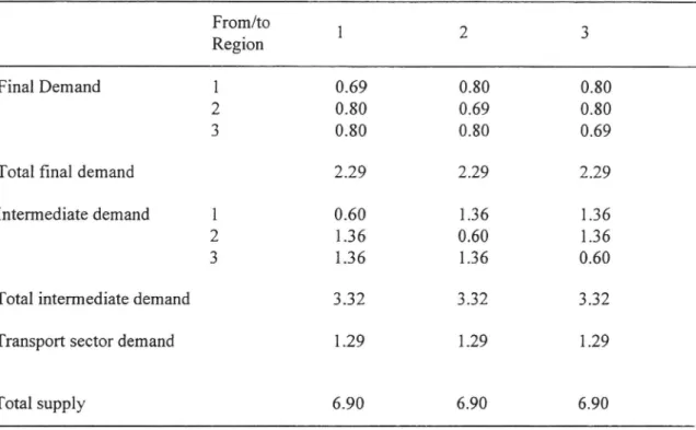
Table 5 below shows the quantity related part of the initial equilibrium. Final demand, intermediate inputs, transport demand and total supply of each good in the pre-improvement case for a unit elasticity of substitution are shown. In this case, nal demand is only about a third of total supply of each commodity. Moreover, due to the limited demand for transportation the demand from the transport sector is also low.

Table 5 Pre improvement demand and supply of goods with a unit elasticity of substitution. From/to 1 2 3 Reglon Final Demand 1 0.69 0.80 0.80 2 0.80 0.69 0.80 3 0.80 0.80 0.69

Total nal demand 2.29 2.29 2.29

Intermediate demand 1 0.60 1.36 1.36

2 1.36 0.60 1.36

3 1.36 1.36 0.60

Total intermediate demand 3.32 3.32 3.32

Transport sector demand 1.29 1.29 1.29

Total supply 6.90 6.90 6.90

In table 6 income and utility relevant variables for three different elasticities . of substitution are given. Since the three regions are equally endowed with technology and labour and have similar preferences, the values are relevant for each region.

Table 6 Wage rates, leisure, incomes and utility indices for the pre-improvement case with different elasticities of substitution.

Elasticity of substitution 1 2 3

Wage rate 1.0 1.0 1.0

Income 120.0 120.0 120.0

Leisure demand 23.76 23.97 23.98

Utility level _ 1.51 6.59 8.77

The welfare impact of an increased elasticity of substitution is manifested as an increase in the level of utility, while incomes and the wage rate, given by the numeraire, are unchanged. Obviously may this increase in utility through increased exibility be

compared with the change in utility obtainable by a reduction in the cost of interaction within a given level of exibility.

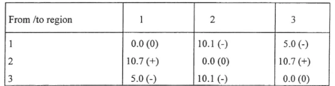
Now, suppose that a transport investment is undertaken on the links between region one and region three. The transport coef cients are reduced by fty percent, which results in a new set of equilibrium unit transport costs as given in table 7.

Table 7 The post-improvement unit transport cost of good i carried to region j with a unit elasticity of substitution. Compare with table 4.

From /to region 1 2 3

1

0.0 (0)

10.1 ()

5.0 ()

2

10.7 (+)

0.0 (0)

10.7 (+)

3

5.0 (_)

10.1 ()

0.0 (0)

A comparison of the post-improvement unit transport cost in table 7 and the corresponding pre-improvement situation in table 4 indicates as expected that the unit transport cost between region one and region three is reduced by more than half of the initial cost. This is due to the fact that the change in transport cost coef cients also reduced the equilibrium prices of the transported goods. The unit transport cost for shipping goods from region two has slightly gone up. This is explained by the increase in the price of good two. The post-improvement prices are shown below.

Table 8 Post-improvement prices with a unit elasticity of substitution. Compare with the pre-improvement situation given in table 4.

REGION 1 2 3

1

33.5 ()

44.0 ()

38.7 ()

2

46.0 (+)

35.5 (+)

46.0 (+)

3

38.7 ()

44.0 ()

33.5 ()

pj

33.5 (-)

.

35.5 (+)

33.5 ()

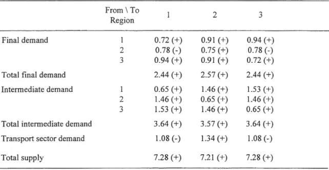
In table 9 the impact of these price changes on ows in the economy are given. The table indicates how the investment in uences inter-regional ows, the transport sector s demand for resources and the equilibrium supply of goods. As a consequence of the increased cost of transportation, the ows of consumer goods from region two has decreased while this region instead consumes more of all goods.

Table 9 Post-improvement demands and equilibrium output of goods with a unit elasticity of substitution. Compare with table 5.

From .\ To 1 2 3

Region

Final demand 1 0.72 (+) 0.91 (+) 0.94 (+)

2

0.78 ()

0.75 (+)

0.78 (-)

3

0.94 (+)

091 (+)

072 (+)

Total nal demand

2.44 (+)

2.57 (+)

2.44 (+)

Intermediate demand l 0.65 (+) 1.46 (+) 1.53 (+)

2

1.46 (+)

0.65 (+)

1.46 (+)

3

1.53 (+)

1.46 (+)

0.65 (+)

Total intermediate demand 3.64 (+) 3.57 (+) 3.64 (+) Transport sector demand 1.08 (-) 1.34 (+) 1.08 (-)

Total supply

7-28 (+)

7-21 (+)

7-28 (+)

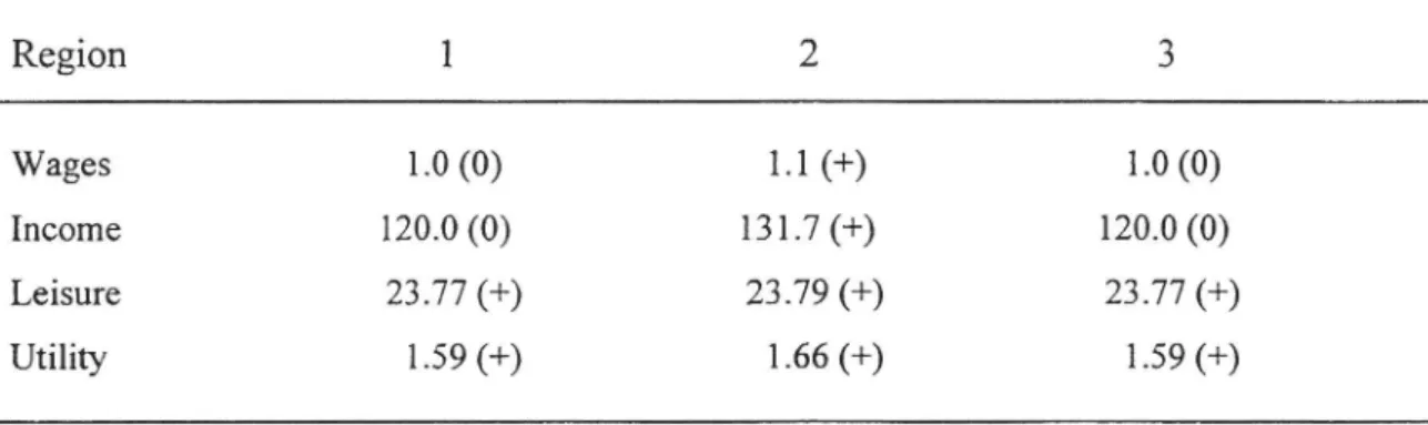
However, both region one and three increase their nal demand since they now have to spend less resources on transport services. On the other hand, ows of intermediate inputs have increased due to the transport improvement. This increase may be explained by the relative reduction in the prices of intermediate inputs as compared to the cost of labour. Changes in labour supply, wage rates, incomes and utilities are given in table 10 below.

Each region improve its utility as a result of the transport cost reduction although the improvement never gives utility increases in parity with those obtained by an increased

exibility in the economy.

Table 10 Post-improvement wages, leisure demand, consumer incomes and utility indices with a unit elasticity of substitution. Compare with the pre improvement outcome in column one of table 6.

Region 1 2 3

Wages 1.0 (O) 1.1 (+) 1.0 (0)

Income 120.0 (O) 131.7 (+) 120.0 (O) Leisure 23.77 (+) 23.79 (+) 23.77 (+) Utility 1.59 (+) 1.66 (+) 1.59 (+)

The average increase in utility from the investment amounts to 6.8 percent. However, especially region two, the one not located at the improved route, had a welfare impact (9.9 percent) which is above what were obtained in the two regions directly located at the route (5.3 percent). This paradoxical observation is in a sharp contrast to a simulation with a more flexible economy. In that case, although all regions improved their welfare, regions directly affected by the improvement bene ted most.

The explanation of this paradox is related to the increased wage in region two. The reduced inter-regional demand for good two tends to move the price of this good upward. The wage rate in region two has to adjust to induce local consumption in order to clear the factor market. With this increase in income, region two consumes more of its own good and of leisure. Given the unit elasticity, the utility from this increase of income outweighs the negative effect of the price increase for the household in region

two.

As was shown, increased exibility gives higher levels of utility in all regions. However, the percentage change in utility in response to an infrastructure investment is largest in the least flexible economy. Hence, a exible economy may always adjust to an inferior transport infrastructure and by this reduce the needfor and the bene ts of an

improvement.

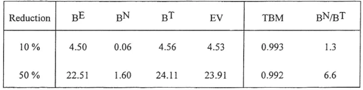
Although this gives interesting results regarding the activity in the spatial economy, our main interest here is the relation between bene ts to traf c and bene ts to the economy in the rst-best case. We have analysed both ten and fty per cent reductions in the transport cost coef cients. In order to examine the impact of the substitution elasticity, similar analyses are performed for different values of the elasticity. The results of our bene t calculations for a unit elasticity are given in table 11 below.

Table 11 Measures of bene ts of improvements between regions one and three. A rst-best economy with a unit elasticity of substitution.

Reduction

BE

BN

BT

EV

TBM

BN/BT

10 %

4.50

0.06

4.56

4.53

0.993

1.3

50 %

22.51

1.60

24.11

23.91

0.992

6.6

The table indicates that independent of the size of improvement EV almost exactly equals the traf c bene t measure BT. The small deviation between the two bene t measures obtained in the TBM may as discussed earlier be explained by the fact that bene ts to traf c only provides an approximation of the exact bene t measure. Hence, we have con rmed that in the rst-best economy total welfare gains of small as well as large scale transport improvements are captured by the full bene ts to traf c on the improved route.

The absolute size of the bene ts varies directly with the scale of improvement. As expected, the share of the bene ts associated with newly generated traf c relative to total traf c bene ts also increases with the size of the investment as is shown by the

BN/BT percentage ratio between generated traf c bene ts and total bene ts in table 11.

The bene ts due to newly generated traf c from a ten per cent reduction, represents little more than one per cent of the total transport cost saving. For a fty percent reduction this ratio increases to above six per cent.

Moreover, the percentage ratio of EV to the total xed labour endowment (EV/L) increases for a large scale investment and, although not shown here, decreases for higher values of the elasticity of substitution. The result is in line with our previous nding that the transport investment produces relatively less bene ts in a more exible economy. The most important result, however, derives from the signi cance of welfare gains associated with newly generated traf c. Although TBM maintains its unit value, the importance of newly generated traf c substantially increases with a large scale transport

investment. By omitting new traf c we will underestimate the bene ts from the

investment by six percent in this case ofa large investment.

5 THE CASE OF INCREASING RETURNS TO SCALE

With increasing returns to scale, the average total cost curve will have a negative slope and a market solution will give a monopoly solution. The monopoly will set the price above marginal cost in order to maximise pro ts. In case the monopoly is forced to set price equal to marginal cost, below average total cost, an Operational loss is obtained. Here, the monopoly is regulated to set it s price equal to its average total cost in order to exclude the need to introduce public transfers or pro ts in the model. We examine how welfare gains of a transport investment change with this deviation from marginal cost pricing. Increasing returns to scale are introduced through the scale parameter in the production function which is set equal to 1.2 for the relevant producers.

Our analysis shows that the impact of positive returns to scale depends on the way transport costs are speci ed. In the rst best case they were proportional to the price of the transported good. The unit transport cost then became a reasonable proportion of the price of the good. However, under a monopoly, the unit transport cost will be set by the price level determined by economies of scale and the TBM becomes conditional on this. In order to evaluate the size of this impact our analysis is initially made with the producer price in the transport cost function based on average cost, named alternative (AI), and secondly by use of the marginal cost of the good produced with increasing returns, i.e. alternative (All).

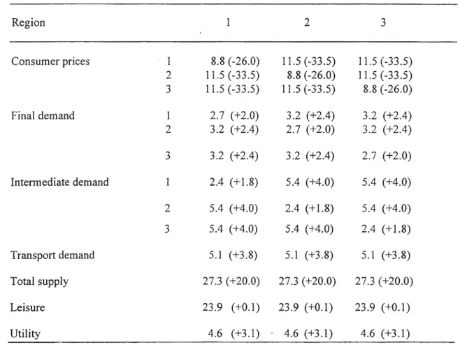
Table 12 Pre investment equilibrium with increasing returns to scale based on transport price (AI) and a unit elasticity of substitution. Figures in brackets give the deviation from the rst-best case in tables 4-6.

Region l 2 3 Consumer prices ' l 8.8 (-26.0) 11.5 ( 33.5) 11.5 (-33.5)

2

11.5 (-33.5)

8.8 (-26.0)

11.5 (33.5)

3

11.5 (33.5)

11.5 (33.5)

8.8 (-26.0)

Final demand

1

2.7 (+20)

3.2 (+24)

3.2 (+24)

2

3.2 (+24)

2.7 (+20)

3.2 (+24)

3

3.2 (+24)

3.2 (+24)

2.7 (+20)

2

5.4 (+40)

2.4 (+1.8)

5.4 (+40)

3

5.4 (+40)

5.4 (+40)

2.4 (+1.8)

Utility

4.6 (+3.1)

4.6 (+3.1)

4.6 (+31)

The pre-investment equilibrium with prices set at average cost (AI) is shown in table 12. As expected, the solution is characterised by considerable price reductions and an increased output as compared to the corresponding rst-best case. Subsequently, a substantial increase in the inter-regional ows are recorded. One may observe that increasing returns to scale has no substantial impact on the demand for leisure as the level of employment in the economy remains almost unchanged. Also in this case, we introduced two levels of infrastructure investments in the economy. The bene t

calculations are summarised below in table 13.

Table 13 Measures of bene ts due to transport improvements with increasing returns to scale, a unit elasticity and transport pricing alternative (AI).

Reduction

BE

BN

BT

EV

TBM

BN/BT

10%

4.50

0.08

4.58

6.55

1.43

1.7

50%

22.50

2.07

24.57

34.95

1.42

8.4

The results in table 13 show that this alternative leads to a considerable discrepancy between traf c bene ts and EV. However, note that transport cost savings for existing traf c remain almost at the same level as in the rst-best model while the ratio of generated traf c bene ts to total transport cost savings has increased. In the case of a fty percent investment it reaches a level of eight percent as compared to six percent achieved in the rst-best case. But the most substantial increase may be observed in the

EV measure.

As the elasticity of substitution is increased the deviation between average total cost and marginal cost declines. Prices are reduced and equilibrium quantities increased. Hence, increased elasticity of substitution has an adverse effect on monopoly pricing, leading to a fall in the bene t multiplier. At a given degree of increasing returns to scale and elasticity of substitution, the size of the transport investment does not seem to have any in uence on the TBM measure although the impact on the magnitude of bene ts obviously is related to the size of the investment.

In transport cost alternative (AI) the transport cost structure was directly affected by the existence of increasing returns to scale in the production of a carried commodity. This may be avoided through approach (AII) where the unit transport cost is proportional to the marginal cost mci of the transported good. Hence, the consumer price in this case is,

Pij-=P,- +mCitij (5-1)

A comparison of the initial equilibrium situations based on (AI) and (All) reveals that prices decline in the second alternative. Consumer prices were reduced by about 12

percent while the commodity ow increases. Nevertheless, the level of employment in

the economy remains at the same level as in case (AI). Despite of the increase in the inter-regional ow, the transport sector s demand for resources decline. This is due to the lower transport cost implied by case (All). Our formulation according to (AII) also gives a higher utility level in each region. The results of a transport improvement based on (AH) is given in table 14 below.

As compared to alternative (AI) the level of traf c bene ts has slightly increased while the equivalent variation has decreased considerably. Thus the true bene t multiplier now takes a much lower value since the unit transport cost is based on the marginal cost of the transported good.

Table 14 Measures of bene ts due to transport improvements with increasing returns to scale and a unit elasticity. Transport costs are calculated according to (All).

Reduction

BE

BN

BT

EV

TBM

BN/BT

10% 4.67 0.07 4.74 5.66 1.20 1.5 50% 23.33 1.82 25.15 29.92 1.19 7.2

Above, we nd that traf c bene ts are still short of EV by about twenty percent but it was forty-three percent in case (AI). Hence, the impact transmitted through the transport sector seems to be rather substantial. Also in this case bene t measures computed for different values of the elasticity of substitution con rm the nding that the size of the true bene t multiplier varies inversely with the level of the elasticity of substitution in the economy.

In the analysis of increasing returns to scale we have so far assumed increasing returns in the production of all goods. However, in a spatial network context this need not be the case. Therefore, we have analysed the case of increasing returns only in region two,

the node not directly located at the improved link, and also the case when increasing

returns only prevails in the two regions making the end points of the improved link. Given that the unit transport cost is defined as (AH) and increasing returns prevail only in the region located away from the improved route, all prices except for the good produced in region two are determined according to marginal cost. In this case the TBM equals one, a result veri ed independently ofthe degree ofthe elasticity ofsubstitution. If the unit transport cost instead is de ned as in (Al), the bene t multiplier only shows a slight deviation from unity. This deviation may, as we discussed earlier, be explained by the fact that the unit transport cost of the good shipped from region two is determined by a price which is not set according to it s marginal cost. This gives an indirect impact on the price of the other goods. Also in this case, the small deviation is removed as the elasticity of substitution is increased in the economy. Our main conclusion thus is that increasing returns in production will have a substantial impact on the benefit multiplier only if the good produced under increasing returns is directly transported on the improved route.

6 CONCLUSIONS

In this paper, we have examined the impact of increasing returns to scale on the relationship between traf c bene ts and economy-wide bene ts in a nontrivial network. The main result is that with increasing returns to scale in all regions, traf c bene ts will underestimate equivalent variation considerably. The deviation between the two measures varies inversely with the elasticity of substitution. However, the deviation between traf c bene ts and equivalent variation does not depend on the size of the improvement. It is although dependent on how transport costs are treated in the model. Moreover, if increasing returns to scale solely prevails in the production of commodities not transported on the improved road while other transported commodities are priced at marginal cost, traf c bene ts either only slightly underestimate equivalent variation or exactly equals EV. The outcome is dependent on the formulation of the transport cost

function.

When all prices are set equal to marginal cost the parity relationship between EV and traf c bene ts holds. The ratio of generated traf c bene ts to transport cost savings for initial traf c in all cases increase with the size of the transport improvement. Hence, in the evaluation of large scale transport investments, an estimation of newly generated traf c is crucial in order to get a realistic assessment of bene ts. Transport cost savings for existing traf c only gives a lower bound of bene ts.

REFERENCES

Dodgson, J.S. (1973) External Effects and Secondary Bene ts in Road Investment Appraisal, Journal of Transport Economics and Policy, pp. 169 185.

Friesz, T., Z-G. Suo and L. Westin (1994) A Spatial Computable General Equilibrium Model. In: Roson. R. ed., Proceedings of the Venice Workshop on Transportation and General Equilibrium Models. Harris, R. (1984) Applied General Equilibrium Analysis of Small Open Economies with Scale

Economies and Imperfect Competition. American Economic Review 74, pp. 1016 32. Hussain, I. (1990) Road Investment Bene ts Over and Above Transport Cost Savings and Gains to

Newly Generated Traf c. Proceedings ofSeminar J Held at the PTRC. Transport and Planning Summer Annual Meeting, University of Sussex, England.

Hussain I. (1996) Bene ts of Transport Infrastructure Investments: A Spatial Computable General Equilibrium Approach. Umeå Economic Studies No 409, Dept. of Economics. Umeå University. Jara-Diaz, S.R. and Friesz, TL. (1982) Measuring the Bene ts Derived from A Transportation

Investment. Transportation Research, Vol. l6B, no. 1, pp. 57-77.

Just, R.H., Hueth, D.L. and Schmitz, A. (1982) Applied Welfare Economics and Public Policy. Prentice-Hall, Englewood Cliffs, NJ. U.S.A.

Kanemoto, Y. and Mera, K. (1985) General equilibrium Analysis of the Bene ts of Large Transportation Improvements, Regional Science and Urban Economics, 15, pp. 343-363

Lesourne, J. (1975) Cost-Bene t Analysis and Economic Theory. North-Holland, Amsterdam. Mohring, H. (1993) Maximizing, Measuring, and not Double Counting Transportation Improvement

Bene ts: A Primer on Closed-and-Open-Economy Cost-Bene t Analysis. Transportation Research Board, Vol. 27B, No. 6, pp. 413-424.

Takayama, T. (1994) Thirty Years with Spatial and Intertemporal economics. The Annals ofRegional Science, 28, pp. 305-322.

Westin, L. (1990a) Vintage Models ofSpatial Structural Change. University of Umeå: Dep. of Economics, Ph.D. thesis. Umeå Economic Studies, No. 227.

Westin, L. (1990b) Location, Transportation and Investments in a Multisector Vintage Model. I: Anselin, L. and M. Madden (eds): New Directions in Regional Analysis, Integrated and Multiregional Approaches. London: Belhaven Press.

UMEÅ ECONOMIC STUDIES

(Studier i nationalekonomi)

All the publications can be ordered from Department of Economics, University of

Umeå, S-90l 87 Umeå, Sweden.

Umeå Economic Studies was initiated in 1972. For a complete list, see Umeå Economic Studies No 366 and earlier.

367 368 369 370 371 372 373 374 375 376 377 378 379

Zhang, Wei-Bin: Growth with Renewable Resources, 1995. Zhang, Wei-Bin: Economic Dynamics with Livestock, 1995 .

Zhang, Wei-Bin: An Agricultural Equilibrium Model with Two Groups, 1995 .

Aronsson, Thomas and Wikström, Magnus: Local Public Expenditures in Sweden.

A Model where the Median Voter is not Necessarily Decisive, 1995.

Aronsson, Thomas, Johansson, Per-Olov and Löfgren, Karl-Gustaf: Investment

Decisions, Future Consumption and Sustainability under Optimal Growth, 1995.

Hultkrantz, Lars: Dynamic Price Response of Inbound Tourism Guest-Nights in

Sweden, 1995.

Brännäs, Kurt and Johansson, Per: Panel Data "Regression for Counts, 1995. Berglund, Elisabet and Brännäs, Kurt: Entry and Exit of Plants: A Study Based on

Swedish Panel Count Data, 1995.

Brännäs, Kurt and Karlsson, Niklas: Endogeneity Testing in Micro Econometric

Models, 1995.

Aronsson, Thomas, Johansson, Per-Olov and Löfgren, Karl-Gustaf: On the Proper

Treatment of Defensive Expenditures in Green NNP Measures, 1995.

Westerlund, Olle: Employment Opportunities, Wages and Interregional Migration in Sweden 1970-1989, 1995.

Axelsson, Roger and Westerlund, Olle: A Panel Study of Migration, Household Real Earnings and Self-Selection, 1995.

Westerlund, Olle: Economic Influences on Migration in Sweden, 1995. PhD thesis.

380 381 382 383 384 385 386 387 388 389 390 391 392 393 394 395

Aronsson, Thomas, Brännlund, Runar and Wikström Magnus: Wage

Determination under Nonlinear Taxes - Estimation and an Application to Panel

Data, 1995.

Brännäs, Kurt: Explanatory Variables in the AR(1) Count Data Model, 1995 . Norén, Ronny: Industrial Transformation in the Open Economy A Multisectoral

View, 1995.

Brännäs, Kurt and Ohlsson, Henry: Asymmetric Cycles and Temporal Aggregation, 1995.

Brännlund, Runar, Chung, Yangho, Päre, Rolf and Grosskopf, Shawna: Emissions Trading and Pro tability: The Swedish Pulp and Paper Industry, 1995 .

Nordström, Jonas: Tourism Satellite Account for Sweden 1992 1993, 1995.

Brännlund, Runar, Löfgren, Karl-Gustaf and Sjöstedt, Sara: Forecasting Prices of

Paper Products: Focusing on the Relation Between Autocorrelation Structure and Economic Theory, 1995.

Qstbye, Stein: Real Options, Wage Bargaining, Regional Subsidies and

Employment, 1995.

Qstbye, Stein: A Real Options Approach to Investment in Factor Demand Models, 1995 .

Bergman, Mats A.: Price Competition under Capacity Constraint with Endogenous Timing of Entry, 1995.

Vredin, Maria: Values of the African Elephant in Relation to Conservation and

Exploitation, 1995.

Bergman, Mats A.: Antitrust, Marketing Cooperatives and Market Power, 1995 . Brännäs, Kurt and Karlsson, Niklas: Estimating the Perceived Tax Scale within a

Labor Supply Model, 1995.

Sjögren, Tomas and Brännäs, Kurt: Recreation Travel Time Conditional on Labour Supply, Work Travel Time and Income, 1995

Löfgren, Karl Gustaf, Nordström, Anna and Nyman, Pär: Willingness to Pay for Work Programs for Disabled Workers, 1995

Backlund, Kenneth, Kriström, Bengt, Löfgren, Karl-Gustaf and Polbring, Eva:

Global Warming and Dynamic Cost-Benefit Analysis Under Uncertainty: An Economic Analysis of Forest Carbon Sequestration, 1995

396 397 398 399 400 401 402 403

404

405

406

407_

408

409

Mortazavi, Reza: Three Papers on the Economics of Recreation, Tourism and

Property Rights, 1995. PhLic thesis

Qstbye, Stein: Regional Labour and Capital Subsidies, 1995. PhD thesis

Bask, Mikael: Dimensions and Lyapunov Exponents from Exchange Rate Series, 1995

Aronsson, Thomas, Backlund, Kenneth and Löfgren, Karl Gustaf: Nuclear Power,

Externalities and Non-Standard Pigouvian Taxes: A Dynamic Analysis under Uncertainty, 1996

Johansson, Per and Brännäs, Kurt: A Household Model for Work Absence, 1996 Löfström, Åsa: Arbetsvärdering i akademin. Hur lönestrukturen kan påverkas i ett

företag som arbetsvärderat, 1996

Zhang, Wei Bin: Knowledge, Infrastructures and Economic Structure, 1996 Zhang, Wei-Bin: Economic Growth, Housing and Residential Location, 1996 Zhang, Wei-Bin: Taste Change, Economic Growth and Structural Transformation,

1996

Brännäs, Kurt, de Gooijer, Jan and Teräsvirta, Timo: Testing Linearity against Nonlinear Moving Average Models, 1996

Bergman, Mats A: Estimating Investment Adjustment Costs and Capital

Depreciation Rates from the Production Function, 1996

Löfström, Åsa: Variation in Female Activity and Employment Patterns: The case of Sweden, 1996

Zhang, Wei Bin: Knowledge and value Economic Structures with Time and Space, 1996.

Hussain Shahid, Imdad: Benefits of Transport Infrastructure Investments: A Spatial Computable General Equilibrium Approach, 1996. PhD thesis.

Eriksson, Maria: Selektion till arbetsmarknadsutbildning, 1996. PhLic thesis. Karlsson, Niklas: Testing for Norrnality in Censored Regressions, 1996

Karlsson, Niklas: Testing for Exponential and Weibull Distributions in Censored Duration Models, 1996

Karlsson, Niklas: Testing and Estimation in Labour Supply and Duration Models, 1996. PhD thesis.

414

Weitzman, Martin L. and Löfgren, Karl-Gustaf: On the Welfare Signi cance of Green Accounting as Taught by Parable, 1996

Aronsson, Thomas and Löfgren, Karl-Gustaf: An Almost Practical Step towards Green Accounting?, 1996

Löfström, Äsa: Can Job Evaluation Improve Women s Wages?, 1996

Axelsson, Roger, Brännäs, Kurt och Löfgren, Karl Gustaf: Arbetsmarknads

utbildning och utförsäkringsgarantin, 1996

Axelsson, Roger, Brännäs, Kurt och Löfgren, Karl-Gustaf: Arbetsmarknadspolitik,

arbetslöshet och arbetslöshetstider under 1990 talets lågkonjunktur, 1996 Li, Chuan-Zhong: Semiparametric Estimation of the Binary Choice Model for

Contingent Valuation, 1996

Li, Chuan-Zhong, Löfgren, Karl-Gustaf and Hanemann, W. Michael: Real Versus

Hypothetical Willingness to Accept. The Bishop and Heberlein Model

Revisited, 1996

Li, Chuan-Zhong and Löfgren, Karl-Gustaf: Renewable Resources and Economic Sustainability. A Dynamic Analysis with Heterogeneous Time Preferences, 1996

Cameron, A. Colin and Johansson, Per: Count Data Regression using Series Expansions: with Applications, 1996

Brännäs, Kurt: Count Data Modelling Measurement Error in Exposure Time, 1996

Bergman, Mats A.: Should Internal Rate of Return, Benefit Cost Ratio, or Present Value Be Used to Evaluate Road and Rail Investments?, 1996

Cassel, Claes-M., Johansson, Per and Palme, Mårten: A Dynamic Discrete Choice Model of Blue Collar Worker Absenteeism in Sweden 1991, 1996

Aronsson, Thomas:Welfare Measurement, Green Accounting and Distortionary Taxes, 1996

Löfgren, Karl Gustaf and Marklund, Per Olov: The Regional Output from Human Capital: Do Universities Matter?, 1996

Olsson, Christina: Chernobyl Effects and Dental Insurance, 1996. PhLic thesis de Luna, Xavier: Projected Polynomial Autoregression for Prediction of

Stationary Time Series, 1997

Persson, Håkan and Westin, Lars: Recursive Transport Flow Dynamics with A Priori Information, 1997

431 Hussain, Imdad and Westin, Lars: Tinbergen Revisited: Benefits from

Infrastructure Investments in an Open Economy, 1997

432 Hussain, Imdad and Westin, Lars: Network Benefits from Transport Investments