Geometric Graphs
Vikrant Ashvinkumar
University of Sydney, Australia vash7242@uni.sydney.edu.auJoachim Gudmundsson
University of Sydney, Australia joachim.gudmundsson@sydney.edu.auChristos Levcopoulos
Lund University, Sweden christos.levcopoulos@cs.lth.seBengt J. Nilsson
Malmö University, Sweden bengt.nilsson.ts@mau.seAndré van Renssen
University of Sydney, Australia andre.vanrenssen@sydney.edu.auAbstract
Online routing in a planar embedded graph is central to a number of fields and has been studied extensively in the literature. For most planar graphs no O(1)-competitive online routing algorithm exists. A notable exception is the Delaunay triangulation for which Bose and Morin [6] showed that there exists an online routing algorithm that is O(1)-competitive. However, a Delaunay triangulation can have Ω(n) vertex degree and a total weight that is a linear factor greater than the weight of a minimum spanning tree.
We show a simple construction, given a set V of n points in the Euclidean plane, of a planar geometric graph on V that has small weight (within a constant factor of the weight of a minimum spanning tree on V ), constant degree, and that admits a local routing strategy that is O(1)-competitive. Moreover, the technique used to bound the weight works generally for any planar geometric graph whilst preserving the admission of an O(1)-competitive routing strategy.
2012 ACM Subject Classification Theory of computation → Design and analysis of algorithms
Keywords and phrases Computational geometry, Spanners, Routing
Digital Object Identifier 10.4230/LIPIcs.ISAAC.2019.30
Related Version A full version of the paper is available at https://arxiv.org/abs/1909.10215.
Funding Joachim Gudmundsson: Funded by the Australian Government through the Australian Research Council DP150101134 and DP180102870.
Christos Levcopoulos: Swedish Research Council grants 2017-03750 and 2018-04001.
1
Introduction
The aim of this paper is to design a graph on V (a finite set of points in the Euclidean plane) that is cheap to build and easy to route on. Consider the problem of finding a route in a geometric graph from a given source vertex s to a given target vertex t. Routing in a geometric graph is a fundamental problem that has received considerable attention in the literature. In the offline setting, when we have full knowledge of the graph, the problem is well-studied and numerous algorithms exist for finding shortest paths (for example, the classic
© Vikrant Ashvinkumar, Joachim Gudmundsson, Christos Levcopoulos, Bengt J. Nilsson, and André van Renssen;
Dijkstra’s Algorithm [9]). In an online setting the problem becomes much more complex. The route is constructed incrementally and at each vertex a local decision has to be taken to decide which vertex to forward the message to. Without knowledge of the full graph, an online routing algorithm cannot identify a shortest path in general; the goal is to follow a path whose length approximates that of the shortest path.
Given a source vertex s, a target vertex t, and a message m, the aim is for an online routing algorithm to send m together with a header h from s to t in a graph G. Initially the algorithm only has knowledge of s, t and the neighbors of s, denoted N (s). Note that it is commonly assumed that for a vertex v, the set N (v) also includes information about the coordinates of the vertices in N (v). Upon receiving a message m and its header h, a vertex
v must select one of its neighbours to forward the message to as a function of h and N (v).
This procedure is repeated until the message reaches the target vertex t. Different routing algorithms are possible depending on the size of h and the part of G that is known to each vertex. Usually, there is a trade-off between the amount of information that is stored in the header and the amount of information that is stored in the vertices.
Bose and Morin [6] showed that greedy routing always reaches the intended destination on Delaunay triangulations. Dhandapani [8] proved that every triangulation can be embedded in such a way that it allows greedy routing and Angelini et al. [1] provided a constructive proof.
However, the above papers only prove that a greedy routing algorithm will succeed on the specific graphs therein. No attention is paid to the quality or competitiveness of the resulting path relative to the shortest path. Bose and Morin [6] showed that many local routing strategies are not competitive but also show how to route competitively in a Delaunay triangulation. Bonichon et al. [3, 4] provided different local routing algorithms for the Delaunay triangulation, decreasing the competitive ratio, and Bonichon et al. [2] designed a competitive routing algorithm for Gabriel triangulations.
To the best of our knowledge most of the existing routing algorithms consider well-known graph classes such as triangulations and Θ-graphs. However, these graphs are generally very expensive to build. Typically, they have high degree (Ω(n)) and the total length of their edges can be as bad as Ω(n) · wt(M ST (V )).
On the other hand, there is a large amount of research on constructing geometric planar graphs with “good” properties. However, none of these have been shown to have all of bounded degree, weight, planarity, and the admission of competitive local routing. Bose et al. [5] come tantalisingly close by providing a local routing algorithm for a plane bounded-degree spanner.
In this paper we consider the problem of constructing a geometric graph of small weight and small degree that guarantees a local routing strategy that is O(1)-competitive. More specifically we show:
Given a set V of n points in the plane, together with two parameters 0 < θ < π/2 and
r > 0, we show how to construct in O(n log n) time a planar ((1 + 1/r) · τ )-spanner with
degree at most 5d2π/θe, and weight at most ((2r + 1) · τ ) times the weight of a minimum spanning tree of V , where τ = 1.998 · max(π/2, π sin(θ/2) + 1). This construction admits an
O(1)-memory deterministic 1-local routing algorithm with a routing ratio of no more than
5.90 · (1 + 1/r) · max(π/2, π sin(θ/2) + 1).
While we focus on our construction, we note that the techniques used to bound the weight of the graph apply generally to any planar geometric graph. In particular, using techniques similar to the ones we use, it may be possible to extend the results by Bose et al. [5] to obtain other routing algorithms for bounded-degree light spanners.
2
Building the Network
Given a Delaunay triangulation DT (V ) of a point set V we will show that one can remove edges from DT (V ) such that the resulting graph BDG(V ) has constant degree and constant stretch-factor. We will also show that the resulting graph has the useful property that for every Delaunay edge (u, v) in the Delaunay triangulation there exists a spanning path along the boundary of the face in BDG(V ) containing u and v. This property will be critical to develop the routing algorithm in Section 3. In Section 4 we will show how to prune BDG(V ) further to guarantee the lightness property.
2.1
Building a Bounded Degree Spanner
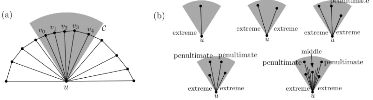
The idea behind the construction is slightly reminiscent to that of the Θ-graph: For a given parameter 0 < θ < π/2, let κ = d2π/θe and let Cu,κbe a set of κ disjoint cones partitioning the plane, with each cone having angle measure at most θ at apex u. Let v0, . . . , vmbe the clockwise-ordered Delaunay neighbours of u within some cone C ∈ Cu,κ(see Figure 1a).
(a) (b)
u u u
u u
extreme extreme extreme extreme extreme
penultimate extreme extreme penultimate penultimate extreme extreme penultimate penultimate middle u v0 v1 v2 v3 v 4 C
Figure 1 (a) An example of the vertices in some cone C with apex u. (b) Extreme, penultimate, and middle are mutually exclusive properties taking precedence in that order.
Call edges uv0 and uvm extreme at u. Call edges uv1 and uvm−1 penultimate at u if
there are two distinct extreme edges at u induced by C. If there are two distinct edges that are extreme at u induced by C and two distinct edges that are penultimate at u induced by C, then, of the remaining edges incident to u and contained in C, the shortest one is called the middle edge at u (see Figure 1b). We emphasise that: (1) If there are fewer than three neighbours of u in the cone C, then there are no penultimate edges induced by C; and (2) If there are fewer than five neighbours of u in the cone C, then there is no middle edge
induced by C.
The construction removes every edge except the extreme, penultimate, and middle ones in every C ∈ Cu,κ, for every point u, in any order. The edges present in the final construction are thus the ones which are either extreme, penultimate, or middle at both of their endpoints (not necessarily the same at each endpoint).
The resulting graph is denoted by BDG(V ). The construction time of this graph is dominated by constructing the Delaunay triangulation, which requires O(n log n) time. Given the Delaunay triangulation, determining which edges to remove takes linear time. The degree of BDG(V ) is bounded by 5κ, since each of the κ cones C ∈ Cu,κcan induce at most five edges. It remains to bound the spanning ratio.
2.2
Spanning Ratio
Before proving that the network is a spanner (Corollary 7) we will need to prove some basic properties regarding the edges in BDG(V ). We start with a simple but crucial observation about consecutive Delaunay neighbours of a vertex u.
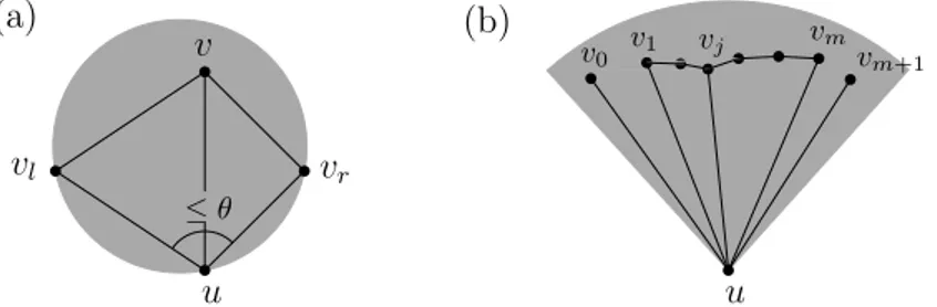
ILemma 1. Let C be a cone with apex u and angle measure 0 < θ < π/2. Let vl, v, vr be
consecutive clockwise-ordered Delaunay neighbours of u contained in C. The interior angle
∠(vl, v, vr) must be at least π − θ.
Proof. In the case when ∠(vl, v, vr) is reflex in the quadrilateral ∆u, vl, v, vr the lemma trivially holds. Let us thus examine the case when ∠(vl, v, vr) is not, in which case the quadrilateral ∆u, vl, v, vris convex. Since vland vrlie in a cone of angle measure θ,∠(vl, u, vr) is at most θ. Consequently, ∠(vl, u, vr) +∠(vl, v, vr) must be at least π (see Figure 2a).
Hence,∠(vl, v, vr) is at least π − θ. J
v
lv
ru
v
≤ θ(a)
(b)
u
v0 v1 vm vm+1 vjFigure 2 (a) Example placement of u, vl, vr and v in the circle ◦(vl, u, vr) (b) The path from v1 to vmalong the hull of u must be in BDG(V ). Furthermore, uv0 and uvm+1are extreme, uv1and uvmare penultimate, and uvjis a middle edge.
This essentially means that∠(vl, v, vr) is wide, and will help us to argue when vlv and
vvrmust be in BDG(V ) (Lemma 5). Next, we define protected edges.
IDefinition 2. An edge uv is protected at u (with respect to some fixed Cu,κ) if it is extreme,
penultimate, or middle at u. An edge uv is fully protected if it is protected at both u and v.
Hence, an edge is contained in BDG(V ) if and only if it is fully protected. We continue with an observation that allows us to argue which edges are fully protected.
IObservation 3. If an edge uviis not extreme at u, then u must have consecutive clockwise-ordered Delaunay neighbours vi−1, vi, vi+1, all in the same cone C ∈ Cu,κ. Similarly, if uvi is neither extreme nor penultimate at u, then u must have consecutive clockwise-ordered Delaunay neighbours vi−2, vi−1, vi, vi+1, vi+2, all in the same cone C ∈ Cu,κ.
I Lemma 4. Every edge that is penultimate or middle at one of its endpoints is fully protected.
Proof. Consider an edge uv that is penultimate or middle at u. Since it is protected at u, we need to show that it is protected at v. Since uv is not extreme at u, u must have consecutive clockwise-ordered Delaunay neighbours vl, v, vrin the same cone by Observation 3.
We show that uv must be extreme at v. Suppose for a contradiction that uv is not extreme at v. Then, by Observation 3, vlv and vvr are contained in the same cone with apex v and angle at most θ < π/2. However, by Lemma 1,∠(vl, v, vr) ≥ π − θ > θ, which is impossible. Thus, uv is extreme at v and protected at v. Hence, the edge is fully protected. J
Now we can argue about the Delaunay edges along the hull of a vertex (see Figure 2b for an illustration of the lemma).
ILemma 5. Let v0, . . . , vm+1be the clockwise-ordered Delaunay neighbours of u contained
in some cone C ∈ Cu,κ. The edges in the path v1, . . . , vm are all fully protected.
Proof. Let vivi+1 be an edge along this path. Suppose for a contradiction that vivi+1 is not protected at vi. It is thus neither extreme, penultimate, nor middle at vi. Then, by Observation 3, viu and vivi−1must be contained in the same cone with apex vias vivi+1. By Lemma 1,∠(vi−1, vi, vi+1) ≥ π − θ > θ, contradicting that vi−1, vi, and vi+1 lie in the same cone. Such an edge must therefore be either extreme or penultimate, and thus protected, at vi≥1. An analogous argument shows that the edge is either extreme or penultimate at
vi+1≤m. It is thus fully protected. J
Since these paths v1, . . . , vmare included in BDG(V ), we can modify the proof of The-orem 3 by Li and Wang [11] to suit our construction to prove that BDG(V ) is a spanner. ITheorem 6. BDG(V ) is a max(π/2, π sin(θ/2) + 1)-spanner of the Delaunay triangulation
DT (V ) for an adjustable parameter 0 < θ < π/2.
Putting the results from this section together, using that the Delaunay triangulation is a 1.998-spanner [12], and observing that BDG(V ) is trivially planar since it is a subgraph of the Delaunay triangulation, we obtain:
ICorollary 7. Given a set V of n points in the plane and a parameter 0 < θ < π/2, one can in O(n log n) time compute a graph BDG(V ) that is a planar τ -spanner having degree at most 5d2π/θe, where τ = 1.998 · max(π/2, π sin(θ/2) + 1).
From the proof of Theorem 6 it follows that for every Delaunay edge (u, v) that is not in BDG(V ), there is a path from u to v along the face containing u and v realising a path of length at most τ · |uv|. This is a key observation that will be used in Section 3.
3
Routing
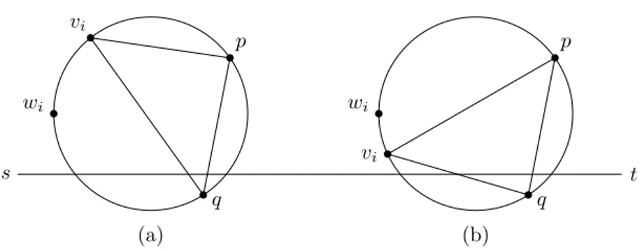
In order to route efficiently on BDG(V ), we modify the local routing algorithm by Bonichon et al. [4]. Given a source s and a destination t on the Delaunay triangulation DT (V ), we assume without loss of generality that the line segment [st] is horizontal with s to the left of t. This routing algorithm then works as follows: when we are at a vertex vi (v0 = s),
set vi+1 to t and terminate if vit is an edge in DT (V ). Otherwise, consider the rightmost
Delaunay triangle Ti= ∆vi, p, q at vi that has a non-empty intersection with [st]. Denote the circumcircle ◦(vi, p, q) with Ci, denote the leftmost point of Ciwith wiand the rightmost intersection of Ci and [st] with ri.
If vi is encountered in the clockwise walk along Ci from wi to ri, set vi+1 to p, the first vertex among {p, q} encountered on this walk starting from vi (see Figure 3a).
Otherwise, set vi+1 to q, the first vertex among {p, q} to be encountered in the counter-clockwise walk along Ci starting from vi (see Figure 3b).
We modify this algorithm in such a way that it no longer necessarily uses the rightmost intersected triangle: At vi>0, we will find a Delaunay triangle Ai based on the Delaunay triangle Ai−1= ∆vi−1, vi, f used in the routing decision at vi−1 (A0= T0).
wi p wi p (a) (b) q q vi vi s t
Figure 3 The routing choice: (a) At viwe follow the edge to p. (b) At viwe follow the edge to q.
Let Ai= ∆vi, p, q be a Delaunay triangle with a non-empty intersection with [st] to the
right of the intersection of Ai−1with [st]. Moreover, if vi is above [st], then, when making a counterclockwise sweep centred at vi starting from vivi−1, we encounter viq before vip, with
viq intersecting [st] and vip not intersecting [st]. An analogous statement holds when vi lies below [st], sweeping in clockwise direction.
We note that these triangles Ai always exist, since the rightmost Delaunay triangle is a candidate. Furthermore, the triangles occur in order along [st] by definition. This implies that the routing algorithm terminates.
ITheorem 8. The modified routing algorithm on the Delaunay triangulation is 1-local and has a routing ratio of at most (1.185043874 + 3π/2) ≈ 5.90.
Proof. The 1-locality follows by construction. The proof for the routing ratio of Bonichon et al.’s routing algorithm [4] holds for our routing algorithm, since the only parts of their proof using the property that Ti is rightmost are:
1. The termination of the algorithm (which we argued above).
2. The categorisation of the Worst Case Circles of Delaunay triangles Ti into three mutually exclusive cases (which we discuss next).
Thus, the modified routing algorithm on the Delaunay triangulation has a routing ratio of at
most (1.185043874 + 3π/2) ≈ 5.90. J
3.1
Worst Case Circles
In the analysis of the routing ratio of Bonichon et al.’s routing algorithm [4], the notion of Worst Case Circles is introduced whereby the length of the path yielded by the algorithm is bounded above by some path consisting of arcs along these Worst Case Circles; this arc-path is then shown to have a routing ratio of 5.90.
Suppose we have a candidate path, and are given a Delaunay triangle ∆vi, vi+1, u intersecting [st]; we denote its circumcircle by Ci with centre Oi. The Worst Case Circle
Ci0 is a circle that goes through vi and vi+1, whose centre Oi0 is obtained by starting at Oi and moving it along the perpendicular bisector of [vivi+1] until either st is tangent to Ci0 or
vi is the leftmost point of Ci0, whichever occurs first. The direction O0i is moved in depends on the routing decision at vi: if vi is encountered on the clockwise walk from wi to ri, then
O0i is moved towards this arc, and otherwise, Oi0 is moved in the opposite direction. Letting
w0
i be the leftmost point of Ci0, we can categorise the Worst Case Circles into the following three mutually exclusive types.
1. Type X1 : vi6= wi0, and [vivi+1] does not cross [st], and st is tangent to Ci0.
2. Type X2 : vi= wi0 and [vivi+1] does not cross [st].
Next, we show that the Worst Case Circles of Delaunay triangles Ai fall into the same categories. Let Ci be the circumcircle of Ai centred at Oi, let wi be the leftmost point of Ci, and let ri be the right intersection of Ci with [st]. We begin with the following observation which follows from how the criteria forces Ai to intersect [st]:
IObservation 9. Let Ai= ∆vi, p, q. Taking a clockwise walk along Cifrom vi to ri, exactly one of p or q is encountered. An analogous statement holds for the counterclockwise walk.
This observation captures the necessary property that allows the categorisation to go through. We denote the Worst Case Circle of Aiby Ci0 with centre Oi0, and leftmost point wi0. ILemma 10. Ci0 can be categorised into the following three mutually exclusive types:
1. Type X1 : vi6= wi0, and [vivi+1] does not cross [st], and st is tangent to Ci0.
2. Type X2 : vi= wi0 and [vivi+1] does not cross [st].
3. Type Y : vi = w0i and [vivi+1] crosses [st].
Proof. If [vivi+1] does not cross [st], Ci0 is clearly of type X1or X2.
Consider when [vivi+1] crosses [st]. Without loss of generality, let vi be above [st] and
vi+1 be below [st]. By Observation 9, vi occurs on the counterclockwise walk around Ci from
wito ri, for if not, neither vertex of Aioccurs on the clockwise walk around Cifrom vi to ri. Since vi is above [st], it lies above the leftmost intersection of Ci with [st] and below wi.
Since O0iis moved along the perpendicular bisector of [vivi+1] towards the counterclockwise arc of vi to vi+1, it must be that wi0 (which starts at wi when Oi0 starts at Oi) moves onto vi
eventually. Thus, Ci0 is Type Y . J
3.2
Routing on BDG(V )
In order to route on BDG(V ), we simulate the algorithm from the previous section. We first prove a property that allows us to distribute edge information over their endpoints. ILemma 11. Every edge uv ∈ DT (V ) is protected by at least one of its endpoints u or v.
Proof. Suppose that uv is not protected at u. Then uv is not extreme at u and thus by Observation 3, u must have consecutive clockwise-ordered Delaunay neighbours vl, v, vr. By Lemma 1, ∠(vl, v, vr) ≥ π − θ > θ since 0 < θ < π/2, and thus vl and vr cannot both belong to the same cone with apex v and angle at most θ. Since vr, u, vl are consecutive clockwise-ordered Delaunay neighbours of v, and vvl and vvr cannot be in the same cone, it follows that vu is extreme at v. Hence, uv is protected at v when it is not protected at u. J This lemma allows us to store all edges of the Delaunay triangulation by distributing them over their endpoints. At each vertex u, we store:
1. Fully protected edges uv, with two additional bits to denote whether it is extreme, penultimate, or middle at u.
2. Semi-protected edges uv (only protected at u), with one additional bit denoting whether the clockwise or counterclockwise face path is a spanning path to v.
We denote this augmented version of BDG(V ) as a Marked Bounded Degree Graph or MBDG(V ) for short. There is only a constant overhead to its construction.
ITheorem 12. MBDG(V ) stores O(1) words of information at each of its vertices.
Proof. There are at most 5κ edges, each with two additional bits, and 2κ semi-protected edges, each with one additional bit, stored at each vertex, where κ is a fixed constant. J
The routing algorithm now works as follows: At a high level, the simulation searches for a suitable candidate triangle Ai at vi. This is done by taking a walk from vi along a face to be defined later, ending at some vertex of Ai. Once at a vertex of Ai, we know the locations of the other vertices of this triangle and thus we can make the routing decision and we route to that vertex. Next, we describe how to route on the non-triangular faces of MBDG(V ).
3.2.1
Unguided Face Walks
Suppose vu1 and vum are a middle edge and a penultimate edge in cone C and suppose that
vu1 is the shorter of the two. For any vertex p on this face, we refer to the spanning face
path from v to p starting with vu1 as an Unguided Face Walk from v to p.
In the simulation, we use Unguided Face Walks in a way that p is undetermined until it is reached; we will take an Unguided Face Walk from v and test at each vertex along this walk if it satisfies some property, ending the walk if it does. Routing in this manner from v to p can easily be done locally: Suppose vu1 was counterclockwise to vum. Then, at any intermediate vertex ui, we take the edge immediately counterclockwise to uiui−1 (v = u0).
The procedure when vu1is clockwise to vumis analogous.
IObservation 13. An Unguided Face Walk needs O(1) memory since at ui, the previous vertex along the walk ui−1 must be stored in order to determine ui+1.
IObservation 14. An Unguided Face Walk from v to p has a stretch factor of at most
max(π/2, π sin(θ/2) + 1) by the proof of Theorem 6.
3.2.2
Guided Face Walks
Suppose vp is extreme at v but not protected at p (i.e., it is a semi-protected edge stored at v). Then, vp is a chord of some face determined by pu1and pumwhere the former is a
middle edge and the latter a penultimate edge. Moreover, recall that we stored a bit with the semi-protected edge vp at v indicating whether to take the edge clockwise or counterclockwise to reach p. We refer to the face path from v to p following the direction pointed to by these bits as the Guided Face Walk from v to p. Routing from v to p can now be done as follows:
1. At v, store p in memory.
2. Until p is reached, if there is an edge to p, take it. Otherwise, take the edge pointed to by the bit of the semi-protected edge to p.
IObservation 15. A Guided Face Walk needs O(1) memory since p needs to be stored in
memory for the duration of the walk.
I Observation 16. A Guided Face Walk from v to p has a stretch factor of at most
max(π/2, π sin(θ/2) + 1) by the proof of Theorem 6.
3.2.3
Simulating the Routing Algorithm
We are now ready to describe the routing algorithm in more detail. First, we consider finding the first vertex after s. If st is an edge, take it and terminate. Otherwise, at s = v0, we
consider all edges protected at s, and let su1and sumbe the first such edge encountered in a counterclockwise and clockwise sweep starting from [st] centred at s. There are two subcases.
(I) If both su1 and sum are not middle edges at s, ∆s, u1, um is a Delaunay triangle
A0. Determine whether to route to u1 or um, using the method described at the start of
Section 3. If the picked edge is fully protected, we follow it. Otherwise, we take the Guided Face Walk from s to this vertex.
(II) If one of su1and sumis a middle edge at s, the other edge must then be a penultimate
edge. Then, A0= ∆s, p, q must be contained in the cone with apex s sweeping clockwise
from su1 to sum. We assume that su1 is shorter than sum. Take the Unguided Face Walk from s until some ui such that ui = p is above [st] and ui+1 = q is below [st]. We have now found A0 = ∆s, p, q and we determine whether to route to p or q, using the method
described at the start of Section 3.
In both cases, the memory used for the Face Walks is cleared and A0 = ∆s, u1, um is stored as the last triangle used.
Next, we focus on how to simulate a routing step from an arbitrary vertex vi. Suppose
vi is above [st], and that Ai−1 is stored in memory. If vit is an edge, take it and terminate. Otherwise, let vif be rightmost edge of Ai−1that intersects [st], and vif be its extension to a line. Make a counterclockwise sweep, centred at vi and starting at vif , through all edges that are protected at vi that lie in the halfplane defined by vif that contains t. Note that
this region must have at least one such edge, since otherwise vif is a convex hull edge, which
cannot be the case since s and t are on opposite sides.
(I) If there is some edge that does not intersect [st] in this sweep, let viu1be the first such
edge encountered in the sweep and let vium be the protected edge immediately clockwise to
viu1 at vi. There are two cases to consider.
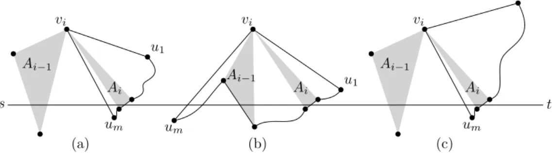
(I.I) If Ai−1is not contained in the cone with apex vi sweeping clockwise from viu1 to
vium(see Figure 4a), simulating the Delaunay routing algorithm is analogous to the method used for the first step: determine if viu1 or vium is a middle edge and use a Guided or Unguided Face Walk to reach the proper vertex of Ai.
u1 (a) um vi Ai−1 Ai s t u1 (b) um vi Ai−1 Ai u1 (c) um vi Ai−1 Ai
Figure 4 The three cases when simulating a step of the routing algorithm: (a) Case I.I, (b) case I.II, and (c) case II.
(I.II) If Ai−1is contained in the cone with apex vi sweeping clockwise from viu1to vium (see Figure 4b), then one of viu1and viummust be a middle edge and the other a penultimate edge, since the edge vif is contained in the interior of this cone. Then, Ai= ∆vi, p, q must be contained in the cone with apex vi sweeping clockwise from viu1 to vif .
We take the Unguided Face Walk, starting from the shorter of viu1 and vium, stopping
when we find some ui such that ui= p is above [st] and ui+1 = q is below [st], and make the decision to complete the Unguided Face Walk to q or not. Note that when starting from
viumwe need to pass f to ensure that Ai lies to the right of Ai−1.
(II) If all of the edges in the sweep intersect [st] (see Figure 4c), let viumbe the last edge encountered in the sweep, and viu1 be the protected edge immediately counterclockwise to it.
Note that Ai−1cannot be contained in this cone, as that would imply that∠(u1, vi, um) ≥ π, making vium a convex hull edge. Simulating the Delaunay routing algorithm is analogous to the method used for the first step: determine if viu1or viumis a middle edge and use a Guided or Unguided Face Walk to reach the proper vertex of Ai.
In all cases, we clear the memory and store Ai= ∆vi, p, q as the previous triangle. The
case where vi lies below [st] is analogous. We obtain the following theorem.
ITheorem 17. The routing algorithm on MBDG(V ) is 1-local, has a routing ratio of at most 5.90 · max(π/2, π sin(θ/2) + 1) and uses O(1) memory.
4
Lightness
In the previous sections we have presented a bounded degree network MBDG(V ) with small spanning ratio that allows for local routing. It remains to show how we can prune this graph even further to guarantee that the resulting network LMBDG(V ) also has low weight.
We will describe a pruning algorithm that takes MBDG(V ) and returns a graph (Light Marked Bounded Degree Graph) LMBDG(V ) ⊆ MBDG(V ), allowing a trade-off between the weight (within a constant times that of the minimum spanning tree of V ) and the (still constant) stretch factor. Then, we show how to route on LMBDG(V ) with a constant routing ratio and constant memory.
4.1
The Levcopoulos and Lingas Protocol
To bound the weight of MBDG(V ), we use the algorithm by Levcopoulos and Lingas [10] with two slight modifications: (1) allow any planar graph as input instead of only Delaunay triangulations, and (2) marking the endpoints of pruned edges to facilitate routing.
At a high level, the algorithm works as follows: Given MBDG(V ), we compute its minimum spanning tree and add these edges to LMBDG(V ). We then take an Euler Tour around the minimum spanning tree, treating it as a degenerate polygon P enclosing V . Finally, we start expanding P towards the convex hull CH(V ). As edges of MBDG(V ) enter the interior of P , we determine whether to add them to LMBDG(V ). This decision depends on a given parameter r > 0. If an edge is excluded from LMBDG(V ), we augment its endpoints with information to facilitate routing should that edge be used in the path found on MBDG(V ). Once P has expanded into CH(V ), we return LMBDG(V ).
Before we bound the weight of LMBDG(V ), we need some new notations. An edge in LMBDG(V ) that belongs to the polygon P , or lies in the interior of P , is called an included
settled edge. If it does not belong to LMBDG(V ), then we say it is an excluded settled edge.
An edge that has not been processed yet by the algorithm is said to be an unsettled edge. Given an unsettled edge uv, let ∂P (u, v) be the path along P from u to v such that
∂P (u, v) concatenated with uv forms a closed curve that does not intersect the interior of P .
When processing an edge uv, it is added to LMBDG(V ) when the summed weight of the edges of ∂P (u, v) is greater than (1 + 1/r) · |uv|. This implies that LMBDG(V ) is a spanner. ITheorem 18. LMBDG(V ) is a (1 + 1/r)-spanner of MBDG(V ) for an adjustable para-meter r > 0.
ITheorem 19. LMBDG(V ) has weight at most (2r + 1) times the weight of the minimum spanning tree of MBDG(V ) for an adjustable parameter r > 0.
Proof. Let P be the polygon that encloses V in the above algorithm. Initially P is the degenerate polygon described by the Euler tour of the minimum spanning tree of V in LMBDG(V ). Give each edge e of P , a starting credit of r|e|. Denote the sum of credits of edges in P with credit(P ). The sum of credit(P ) and the weight of the initially included settled edges is then (2r + 1) times the weight of the minimum spanning tree of MBDG(V ).
As P is expanded and edges are settled, we adjust the credits in the following manner: If an unsettled edge uv is added into LMBDG(V ) when settled, we set the credit of the newly added edge uv of P to credit(∂P (u, v)) − |uv|, and, by removing ∂P (u, v) from P , we effectively set the credit of edges along ∂P (u, v) to 0.
If an unsettled edge is excluded from LMBDG(V ) when settled, we set the credit of the newly added edge uv of P to credit(∂P (u, v)), and, by removing ∂P (u, v), we effectively set the credit of edges along ∂P (u, v) to 0.
We can see that the sum of credit(P ) and the weights of included settled edges, at any time, is at most 2r + 1 times the weight of the minimum spanning tree of MBDG(V ).
It now suffices to show that credit(P ) is never negative, which we do by showing that for every edge uv of P , at any time, credit(uv) ≥ r · weight(uv) ≥ 0. Initially, when
P is the Euler Tour around the minimum spanning tree of MBDG(V ), we have that credit(uv) = r · weight(uv). We now consider two cases.
(I) If uv is added to LMBDG(V ), then credit(uv) equals
credit(∂P (u, v))−|uv| ≥ r ·weight(∂P (u, v))−|uv| ≥ r(1+1/r) |uv|−|uv| = r ·weight(uv).
The first inequality holds from the induction hypothesis, and the second inequality and last equality hold since uv is added to LMBDG(V ).
(II) If uv is not added to LMBDG(V ), then credit(uv) equals
credit(∂P (u, v)) ≥ r · weight(∂P (u, v)) = r · weight(uv).
The first inequality holds by induction, and the equality holds since uv was not added. Since credit(P ) is never negative, and the sum of credit(P ) and the weights of included settled edges is at most 2r + 1 times the weight of the minimum spanning tree of MBDG(V ),
the theorem follows. J
Putting together all the results so far, we get:
I Theorem 20. Given a set V of n points in the plane together with two parameters
0 < θ < π/2 and r > 0, one can compute in O(n log n) time a planar graph LMBDG(V ) that
has degree at most 5 d2π/θe, weight of at most ((2r + 1) · τ ) times that of a minimum spanning tree of V , and is a ((1 + 1/r) · τ )-spanner of V , where τ = 1.998 · max(π/2, π sin(θ/2) + 1).
Proof. Let us start with the running time. The algorithm by Levcopoulos and Lingas (Lemma 3.3 in [10]) can be implemented in linear time and, according to Corollary 7,
BDG(V ) can be constructed in O(n log n) time, hence, O(n log n) in total.
The degree bound and planarity follow immediately from the fact that LMBDG(V ) is a subgraph of MBDG(V ), and the bound on the stretch factor follows from Theorem 18.
It only remains to bound the weight. Callahan and Kosaraju [7] showed that the weight of a minimum spanning tree of a Euclidean graph G(V ) is at most t times that of the weight of M ST (V ) whenever G is a t-spanner on V . Since MBDG(V ) is a τ -spanner on V by Corollary 7, LMBDG(V ) has weight of at most ((2r + 1) · τ ) times that of the minimum spanning tree of V . This concludes the proof of the theorem. J Finally, we prove that LMBDG(V ) has short paths between the ends of pruned edges. ITheorem 21. Let uv be an excluded settled edge. There is a face path in LMBDG(V ) from u to v of length at most (1 + 1/r) · |uv|.
Proof. If uv is the first excluded settled edge processed by the Levcopoulos-Lingas algorithm, then all edges of ∂P (u, v) must be included in LMBDG(V ). By planarity, no edge will be added into the interior of the cycle consisting of uv and ∂P (u, v) once uv is settled, and thus
uv will be a chord on the face in LMBDG(V ) that coincides with ∂P (u, v). Thus, ∂P (u, v) is
a face path in LMBDG(V ) from u to v with a length of at most weight(uv) ≤ (1 + 1/r) · |uv|. Otherwise, if uv is an arbitrary excluded edge, then some edges of ∂P (u, v) may be excluded settled edges. If none are excluded, then ∂P (u, v) is again a face path with length at most weight(uv). However, if some edges are excluded, then, by induction, for each excluded edge pq along ∂P (u, v), there is a face path in LMBDG(V ) from p to q with a length of
weight(pq) ≤ (1 + 1/r) · |pq|. Replacing all such pq in ∂P (u, v) by their face paths, and since
no edge will be added into the interior of the cycle consisting of uv and ∂P (u, v) once uv is settled, ∂P (u, v) with its excluded edges replaced by their face paths is a face path in LMBDG(V ) from u to v with a length of weight(uv) ≤ (1 + 1/r) · |uv|. J
5
Routing on the Light Graph
In order to route on LMBDG(V ), we store an edge at each of its endpoints when it is excluded. Specifically, let uv be some excluded edge, at u (and v) we store uv, along with one bit to indicate whether the starting edge of the (1 + 1/r)-path is the edge clockwise or counterclockwise to uv.
IObservation 22. LMBDG(V ) stores O(1) words of information at each vertex.
To route on LMBDG(V ), we simulate the routing algorithm on MBDG(V ). When this algorithm would follow an excluded edge uv at u, we store v and the orientation of the face path from uv at u in memory. Then, until v is reached, take the edge that is clockwise or counterclockwise to the edge arrived from, in accordance with the orientation stored. Once v is reached, we proceed with the next step of the routing algorithm on MBDG(V ).
Note that bounding the weight in this manner only requires the input graph to be planar. It transforms the pruned edges into O(d) information, where d is the degree of the input graph. This information is then distributed across the vertices of the face, such that each vertex stores O(1) information. The scheme of simulating a particular routing algorithm and switching to a face routing mode when needed can then be applied to the resulting graph. I Lemma 23. The routing algorithm on LMBDG(V ) is 1-local, has a routing ratio of
5.90(1 + 1/r) max(π/2, π sin(θ/2) + 1) and uses O(1) memory.
Proof. The 1-locality follows by construction. The routing ratio follows from Theorem 17. Finally, the memory bound follows from the fact that while routing along a face path to get across a pruned edge, no such subpaths can be encountered. Thus, the only additional memory needed at any point in time is a constant amount to navigate a single face path. J
6
Conclusion
We showed how to construct and route locally on a bounded-degree lightweight spanner. In order to do this, we simulate the Delaunay routing algorithm by Bonichon et al. [4]. A natural question is whether our routing algorithm can be improved by using the improved Delaunay routing algorithm by Bonichon et al. [3]. Unfortunately, this is not obvious: when applying the improved algorithm on our graph, we noticed that the algorithm can revisit vertices. While this may not be a problem, it implies that the routing ratio proof from [3] needs to be modified in a non-trivial way and thus we leave this as future work.
References
1 Patrizio Angelini, Fabrizio Frati, and Luca Grilli. An Algorithm to Construct Greedy Drawings of Triangulations. Journal of Graph Algorithms and Applications, 14(1):19–51, 2010.
2 Nicolas Bonichon, Prosenjit Bose, Paz Carmi, Irina Kostitsyna, Anna Lubiw, and Sander Verdonschot. Gabriel triangulations and angle-monotone graphs: Local routing and recognition. In International Symposium on Graph Drawing and Network Visualization (GD), pages 519–531, 2016.
3 Nicolas Bonichon, Prosenjit Bose, Jean-Lou De Carufel, Vincent Despré, Darryl Hill, and Michiel Smid. Improved routing on the Delaunay triangulation. In Proceedings of the 26th Annual European Symposium on Algorithms (ESA), 2018.
4 Nicolas Bonichon, Prosenjit Bose, Jean-Lou De Carufel, Ljubomir Perković, and André Van Renssen. Upper and lower bounds for online routing on Delaunay triangulations. Discrete & Computational Geometry, 58(2):482–504, 2017.
5 Prosenjit Bose, Rolf Fagerberg, André van Renssen, and Sander Verdonschot. Optimal Local Routing on Delaunay Triangulations Defined by Empty Equilateral Triangles. SIAM Journal on Computing, 44(6):1626–1649, 2015.
6 Prosenjit Bose and Pat Morin. Online routing in triangulations. SIAM Journal on Computing, 33(4):937–951, 2004.
7 Paul B. Callahan and S. Rao Kosaraju. Faster algorithms for some geometric graph problems in higher dimensions. In Proceedings of the 4th ACM-SIAM Symposium on Discrete Algorithms (SODA), pages 291–300, 1993.
8 Raghavan Dhandapani. Greedy Drawings of Triangulations. Discrete & Computational Geometry, 43(2):375–392, 2010.
9 Edgar W. Dijkstra. A Note on Two Problems in Connexion with Graphs. Numerische Mathematik, 1:269–271, 1959.
10 Christos Levcopoulos and Andrzej Lingas. There are planar graphs almost as good as the complete graphs and almost as cheap as minimum spanning trees. Algorithmica, 8(1-6):251–256, 1992.
11 Xiang-Yang Li and Yu Wang. Efficient construction of low weight bounded degree planar spanner. In Proceedings of the 9th Annual International Computing and Combinatorics Conference (COCOON), pages 374–384. Springer, 2003.
12 Ge Xia. The stretch factor of the Delaunay triangulation is less than 1.998. SIAM Journal on Computing, 42(4):1620–1659, 2013.