Department of Wildlife, Fish, and Environmental Studies
Beavers and environmental flow
– the contribution of beaver dams to flood
and drought prevention
Beavers and environmental flow – the contribution of beaver
dams to
Wali Uz Zaman
Supervisor: Frauke Ecke, Swedish University of Agricultural Sciences, Department of Wildlife, Fish, and Environmental Studies
Assistant supervisor: Jörn Pagel, University of Hohenheim, Landscape Ecology and Vegetation Science
Examiner: Navinder Singh, Swedish University of Agricultural Sciences, Department of Wildlife, Fish, and Environmental Studies
Credits: 30 credits
Level: Second cycle, A2E
Course title: Master Thesis in Environmental science, A2E –
Management of Fish and Wildlife Populations – Master’s Programme
Course code: EX0936
Course coordinating department: Department of Wildlife, Fish, and Environmental Studies Place of publication: Umeå
Year of publication: 2019
Cover picture: From GIS software
Title of series: Examensarbete/Master's thesis
Part number: 2019:17
Online publication: https://stud.epsilon.slu.se
Keywords: beaver dam, beaver pond, environmental flow, flood, drought, GIS
Swedish University of Agricultural Sciences Faculty of Forest Sciences
Before they were driven to near extinction, beavers populated the smaller rivers in Europe, Asia and North America. They are ecosystem engineers, since their dam building activities have a cascading effect on biogeochemistry, hydrology, ecosystem structure as well as biodiversity of the affected and surrounding area. I studied using a GIS (geographic information system) software whether dams built by beavers play a role in preventing drought in their surrounding area, and preventing flood down-stream from their location. In the analyses, I combined identified beaver systems and digital elevation models to quantify the carrying capacity of beaver ponds. The Råne River catchment in northern Sweden was the study area. The mean area of the beaver ponds that were identified in the Råne River catchment are 3080 m2 with a standard
error of 241 m2, with a total of 313 identified dams resulting in a total surface area of
beaver ponds of 964124 m2.
Keywords: beaver dam, beaver pond, environmental flow, flood, drought, GIS
List of tables 6 List of figures 7 Abbreviations 8 1 Background 9 2 Objective 12 3 Methodology 13 3.1 Study Area 13
3.2 Identification of Beaver Dams 15
3.3 Spatial Analysis 17 4 Results 21 4.1 Identified Ponds 22 4.2 Simulated Ponds 24 5 Discussion 27 6 Conclusion 29 References 30 Acknowledgements 32
Table of contents
Table 1. Land cover types present in the Råne River catchment 13 Table 2. Area distribution of lakes in the catchment area of Råne River 15 Table 3. Statistical information (area) of the distribution of identified dams 23 Table 4. Statistical information (estimated volume) of the distribution of identified
dams 24
Table 5. Statistical information (area) of the distribution of simulated dams 25 Table 6. Statistical information (estimated volume) of the distribution of simulated
dams 26
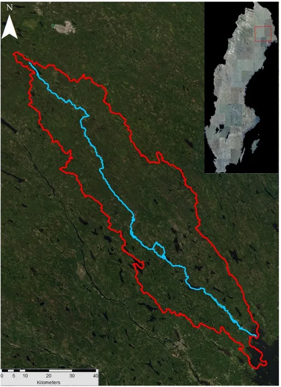
Figure 1. Project area showing the Råne River and the catchment area (red border) 14
Figure 2. Beaver system on orthophotograph 16
Figure 3. Simulated beaver pond 18
Figure 4. Pond created by a beaver dam 19
Figure 5. Methodology flow chart for the analysis of beaver systems in the Råne River
catch-ment.
Figure 6. Map showing the dams that were identified on the orthophotograph (n = 313) 21
Figure 7. Map showing the simulated dams (n = 310) 22
Figure 8. Frequency distribution of the surface area of (n = 313) identified beaver dams in
the Råne River catchment. 23
Figure 9. Frequency distribution of the estimated volume of (n = 313) identified beaver
dams in the Råne River catchment. 24
Figure 10. Frequency distribution of the surface area of (n = 310) simulated beaver dams
in the Råne River catchment. 25
Figure 11. Frequency distribution of the estimated volume of (n = 310) simulated beaver
dams in the Råne River catchment. 26
List of figures
ca. circa
CRV corrected raster value DEM digital elevation model
GIS Geographic Information System ha hectares
IPCC International Panel for Climate Change km2 square kilometres
m2 square metres
m3 cubic metres
SMHI Swedish Meteorological and Hydrological Institute WGS World Geodetic System
Beavers are one of the most prominent representatives of ecosystem engineers (Jones et al. 1994) due to their dam building activities, which has cascading effects on biogeochemistry, hydrology, ecosystem structure as well as biodiversity (Naiman et al. 1988). Lake- or stream living beavers that don’t build dams can have a major impact on local tree species composition, plant succession and sediment dynamics (Moore 2006). Dam-building creates ponds as protection against preda-tors such as coyotes, wolves, and bears, and provides easy and protected access to food throughout the whole year. Building dams in areas with shallow, slow flowing water also prevents the blockage of the underwater entrance to their lodges by ice in winter and also prevents predators from entering the lodge. The effects of dam building are what distinguishes beavers from most other ecosystem engineers; the damming alters the environment both locally (the scale of engineering activity), and potentially at the scale of entire catchments or even landscapes. Beavers play a fun-damental role in community structure and their removal results in comprehensive alterations of ecosystem processes and functioning (Jones et al. 1994). Hence, as beavers affect their abiotic and biotic environment in such a way, they are consid-ered to be keystone species
Dam construction converts stream sections into ponds upstream of the dam, in-creasing both the upstream water volume and area and dein-creasing velocity (re-viewed by Ecke et al. 2017). This conversion significantly reduces the length ratio between stream like (lotic) and lake like (lentic) stream sections (Andersen and Shafroth 2010). The extent of the hydrological effect largely depends on the geo-morphology of the dammed area (Johnston and Naiman 1987). In flat areas, the increase in water volume increases both flood risk and the increase in water table in productive forests or agricultural areas might result in subsequent significant eco-nomic loss (Bhat et al. 1993; Sund 2009). Hydrological effects are not restricted to upstream areas. A significant amount of water bypasses beaver dams, increasing surface runoff and groundwater seepage (Westbrook et al. 2006). By increasing wa-ter retention in low order streams, beavers provide the so far largely underestimated
ecosystem service of flood control downstream in the catchment (Puttock et al. 2017). In analogy, the collapse of a beaver dam increases flooding risk downstream (Andersen and Shafroth 2010), an effect that might be mitigated by the presence of cascades of beaver dams.
When building dams, beavers first fell the trees near the river or stream to block its flow and create a diversion. Branches and logs are then driven into the mud of the stream bed to form a base, afterwards sticks, bark, rocks, mud, grass, leaves, masses of plants, and anything else available, are used to build the superstructure (Muller and Watling 2016). The dams are usually below 1.5 m in height (Muller and Watling 2016), and can be as long as 850 m and wide as 46 m (depends on the river). A 1.4 m high dam can withstand a flow volume of up to 1.34 m3/s per meter of width
(Muller and Watling 2016).
According to Naiman et al. (1988), beaver impounded landscapes can be grouped under eight general categories; open water, seasonally flooded, bog, marsh, dead woody, deciduous woody, not impounded lake, and not impounded upland. Some of these types resist change while others are altered rapidly and abandoned by beavers. Open water, seasonally flooded, and marsh types are dynamic, and are re-placed by one another in a beaver-pond abandonment cycle; a process that often takes more than 10 years (Naiman et al. 1988).
After abandoning a pond, beavers will look for another area with suitable food sources, and once they find such an area, they may start building a new dam there, or, they will occupy an empty dam, if one is present in the area (Naiman et al. 1988). A beaver family consists of an adult male and adult female in a monogamous pair and their kits and yearlings. The number of members in the family can be as high as ten, excluding the parent beavers. Groups of beavers with such high numbers build more than one lodges, while smaller groups build only one (Dietland and Lix-ing 2003).
Beavers became almost continent-wide extirpated with resulting absence in most European countries for more than 100 years and lack of ecological impact for prob-ably almost 200 years. Beavers in Sweden were hunted to extinction by approxi-mately 1870 (Salvensen 1928). In 1922, two beavers were bought from Norway and reintroduced in the province of Jämtland in Sweden; between 1922 and 1939, about 80 Norwegian beavers were reintroduced at 19 different sites in Sweden (Hartman 2002). The population of beavers was estimated to be ca. 100,000 in Sweden ac-cording to Hartman (1999).
Due to climate change, areas which already suffer from annual droughts or floods might be faced with stronger and/or more prolonged ones in the future. In the North-ern Hemisphere, both frequency and extent of extreme weather events are predicted to increase (IPCC2014; Pecl et al. 2017). During summer, this will be in the form of longer periods of high temperatures combined with low precipitation (Francis
and Skific 2015), increasing the risk for droughts. During winter, higher frequency of rain is expected (Post et al. 2009), which increases flood risk. Therefore, under the scenarios of drier summer climate, beavers might contribute to maintain ground-water levels or to mitigate its decrease (see also Hood and Bayley 2008). In regions with expected increased precipitation, cascades of beaver dams might mitigate floods downstream.
The aim of the thesis is to investigate whether beaver dams can mitigate floods and drought and to what extent. Therefore, I studied the following question:
1. What is the water carrying capacity of beaver ponds?
By looking at the water carrying capacity, I hypothesize that beaver dams can significantly increase the open water area and the water volume in the catchment.
3.1 Study
Area
In my project, I focused on the Råne River (Swedish: Råneälven) that runs through the county of Norrbotten in northern Sweden (Figure 1). The source of the river is the Råneträsket (Radnejaure) located around 66.92340°N 20.57080°E (WGS 84), around the center of Norrbotten county, and flows into the Bothnian Bay with an average discharge of 43.4 m3/s (SMHI), with a total downstream distance of 1927
km (Swedish Agency for Marine and Water Management). The basin of the river is 4207.3 km2 in area (SMHI).
The river covers a variety of landscape types; forests, wetlands, lakes, agricul-tural lands, open areas and small towns (Swedish Agency for Marine and Water Management) (Table 1).
Table 1. Land cover types present in the Råne River catchment
Land cover type Area
(km2) Percentage of total (%) Agricultural lands 40.11 0.95 Small towns 5.90 0.14 Forests 2857.55 67.92 Open lands 9.33 0.22 Wetlands 1114.44 26.49 Water 178.23 4.24
Other landscape types 1 1.68 0.04
1 urban areas, mountains and glaciers. Source: Swedish Agency for Marine and Water Management.
3 Methodology
Figure 1. Project area showing the Råne River and the catchment area (red border)
The lakes in the catchment area of the Råne River are predominantly small (0.1 km2 or less in area), while larger lakes (sized 10 km2 and above) are rare (Table 2).
Table 2. Area distribution of lakes in the catchment area of Råne River
Lake (area class)1 Number
A (>100 km2) 0
B (10-100 km2) 2
C (1-10 km2) 27
D (0.1-1 km2) 204
E (<0.1 km2) 561
1 The classes are in accordance to the area classes set by SVAR, a division of the Swedish National
Archives Source: Swedish Agency for Marine and Water Management
3.2 Identification
of Beaver Dams
Beaver dams and beaver systems can be identified on aerial photographs and on satellite images (Martin et al. 2015; Puttock et al. 2015). For my study, I used an orthophotograph (or orthophoto) to help identify beaver dams within the Råne River catchment. An orthophotograph is an aerial image that has been geometrically cor-rected so that the image is uniform from edge to edge to remove terrain effects and distortions caused when taking the picture.
I loaded the orthophotograph from the GIS server of The Swedish University of Agricultural Sciences (SLU). The orthophotograph had a resolution of 1 m and was from the year 2014. I used the orthophotograph together with a shapefile showing the location of potential beaver systems (F. Ecke, personal communication), to iden-tify the location of beaver dams within the Råne River catchment, i.e. including the Råne River and its tributaries and distributaries (Figure 2). A beaver system can consist of several dams; usually the beavers use one to divert the flow of a river to create a pond, and another one for habitation. I created a new shapefile (named PDams) to record the location of beaver dams and for each identified dam, I as-signed its accuracy at two levels (high accuracy or inferred) using the position of the beaver systems. High accuracy means that the dam and the ponds nearby were visible in the orthophotograph, whereas inferred refers to when I located dams with the help of a river network shapefile.
3.3 Spatial
Analysis
Once I finalized the identification process, I created a polygon shapefile to extract the study area from the orthophotograph with the help of the “Extract by Mask” tool under the Spatial Analyst toolbox in ArcGIS v10.6 (ESRI 2018). Once I extracted the raster image file from the orthophotograph, and named it “Project Area”, I cre-ated a digital elevation model (DEM) from the “Project Area” raster image file, in this case a slope DEM with the help of the “Slope” tool under the Spatial Analyst toolbox (ArcGIS 10.6, 2018).
After creating the slope DEM, I used the “Fill” tool under Spatial Analyst toolbox to remove any small inaccuracies in the DEM data, e.g. values that were abnormally high or low for data, or even errors (values like 9999 and negative val-ues). I used the fill tool in batches, as using the tool on the whole DEM made the process slow and worked at a scale of 1:40000, a total of 135 smaller “Fill” raster images were created. Once the all the “Fill” raster files were created, I created “Flow Direction” raster files using the “Flow Direction” tool under Spatial Analyst toolbox from all 135 “Fill “images followed by the creation of “Flow Accumulation” raster image files from the 135 “Flow Direction” raster images with the help of “Flow Accumulation” tool under the Spatial Analyst toolbox.
The 135 “Flow Direction” images were then used to create one combined “Flow Direction” raster image with the help of “Mosaic to New Raster” tool under the Data Management toolbox; the 135 “Flow Accumulation” raster images were combined to create one “Flow Accumulation” image using the same tool.
I then, extracted the elevation data from the DEM using the PDams shapefile using the tool “Extract Multi Values to Points” tool. Once the elevation data were extracted (the field was titled “RASTERVALUE”, I created a field in the attribute table of the PDams shapefile named CRV (corrected raster value); this field con-tained elevation information including dam height. It was calculated using the “Field Calculator” tool as follows
CRV = RASTERVALUE + 1.5
The 1.5 indicates the applied height of beaver dams in meters.
Using the “Flow Accumulation” and “Flow Direction” raster image files and the PDams shapefile (with elevation data), I created a model to find the watersheds cre-ated by each dam. This model made use of the “Snap Pour Point” and the “Water-shed” tools.
The “Snap Pour Point” tool used the Flow Accumulation map and PDams point shapefile to identify pour points, i.e., points where the water accumulates. This “Pour Point” data is then automatically used in combination with the Flow Direction raster to identify the watershed(s) (water accumulation area) around the pour points.
I have individually identified the watersheds for each dam (313 using PDams shape-file) I have identified, and combined all the 313 watershed images into one water-shed map using the “Mosaic to New Raster” tool (file named PDamsws).
When food sources are depleted, beavers abandon their territory and establish new systems either up- or downstream of their present location. To simulate such temporal dynamics in the presence and distribution of beavers, I identified stream stretches where beavers potentially may shift to in the future after abandoning their current systems. For this simulation, I used stream stretches rich in trees visible on the orthophotograph as a criterion, this is shown in Figure 3. I stored the simulated beaver systems in a shapefile called SDams.
Once all simulated dams were in place, I ran the model for creating pour points and watersheds again for the SDams point shapefile (310 watersheds identified), and combined 310 identified watershed images using “Mosaic to New Raster” tool (file named SDamsws). Then I converted the two watershed (PDamsws and SDamsws) images into two polygon shapefiles (named PDamsWS and SDamsWS respectively) using the “From Raster to Polygon” conversion tool.
Once the polygon shapefiles were created, I added a field in the attribute table of each shapefile to calculate the area of each polygon, using the “Calculate Geometry” option.
Figure 4. Pond created by a beaver dam
Figure 4 illustrates a watershed.
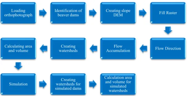
Figure 5. Methodology flow chart for the analysis of beaver systems in the Råne River catchment.
The volume would have been a very good addition as it would give us the exact amount of water being held by the dams, however, as there were many zero and negative values they could not be used here. Hence, I estimated the volumes of the ponds by modelling them to be cuboids; using the area and the height of the dams to be 1.5 meters (as used in my Corrected Raster Value calculation).
Volume of pond = Area of pond x 1.5 m
I converted the attribute table for both the identified and simulated dam shape-files into an MS Excel file using a conversion tool, and then transferred the “Area” column to a text file and used R Studio v3.5 (RStudio Team 2018) to calculate the summary statistics of the data and create histograms.
Loading
orthophotograph Identification of beaver dams Creating slope DEM Fill Raster
Flow Direction Flow Accumulation Creating watersheds Calculating area and volume
Simulation watersheds for Creating
simulated dams
Calculation area and volume for
simulated watersheds
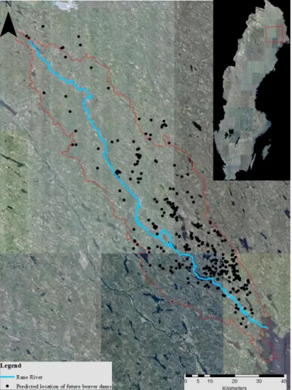
Two sets of beaver pond watershed data were generated; 313 beaver ponds for the identified beaver dams, and 310 beaver ponds for the simulated beaver dams. The watersheds identified in my study correspond to the ponds created by beaver dams. Figures 6 and 7 show the distribution of the identified and simulated ponds respec-tively.
Figure 6. Map showing the dams that were identified on the orthophotograph (n = 313)
Figure 7. Map showing the simulated dams (n = 310)
4.1 Identified
Ponds
The total area of the identified ponds is 964123.98 m2 and the total estimated volume
is 1446185.97 m3. Most of the dams could retain water in an area of less than 5000
m2 and comparatively fewer could retain water in an area of over 5000 m2 (Figure
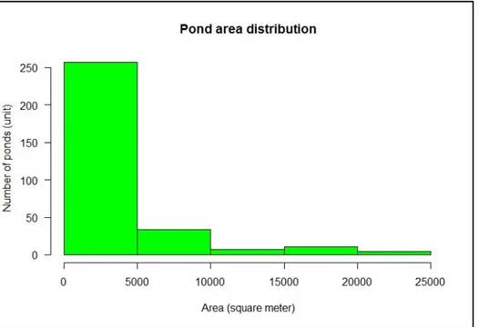
Figure 8. Frequency distribution of the surface area of (n = 313) identified beaver dams in the Råne
River catchment.
As Figure 8 shows, there are rarely any beaver ponds with an area over 20000 m2. From the graph it can be assumed that the median and mean areas are in between
125.20 and 10000 m2. Table 3 summarizes the statistical information.
Table 3. Statistical information (area) of the distribution of identified dams
Statistical operator Value (m2)
Minimum 125.20
Median 1417.70
Mean (including error) 3079.95 ± 240.60
Maximum 21538.27
Figure 9 shows the distribution of estimated volumes of the ponds created by the beaver dams identified in the orthophotograph.
Figure 9. Frequency distribution of the estimated volume of (n = 313) identified beaver dams in the
Råne River catchment.
As Figure 9 shows, there are rarely any beaver ponds with volume over 20000 m3, with the least being between 20000 and 25000 m3. From the graph it can be
guessed that the median and mean volumes are in between 187.80 and 10000 m2.
Table 4 summarizes the statistical information.
Table 4. Statistical information (estimated volume) of the distribution of identified dams
Statistical operator Value (m3)
Minimum 187.80
Median 2126.60
Mean (including error) 4620.40 ± 360.88
Maximum 32307.40
4.2 Simulated
Ponds
The total area of the simulated beaver ponds in the catchment was 2348824.09 m2
Figure 10. Frequency distribution of the surface area of (n = 310) simulated beaver dams in the Råne
River catchment.
As Figure 10 shows, there were few beaver ponds with an area over 20000 m2.
However, the distribution is more uniform, unlike the case with the identified dams. Table 5 summarizes the statistical information.
Table 5. Statistical information (area) of the distribution of simulated dams
Statistical operator Value (m2)
Minimum 104.60
Median 7231.50
Mean (including error) 7576.90 ± 241.76
Maximum 23354.30
Figure 11 shows the distribution of estimated volumes of the ponds created by the simulated beaver dams.
Figure 11. Frequency distribution of the estimated volume of (n = 310) simulated beaver dams in the
Råne River catchment.
As Figure 11 shows, there were rarely any beaver ponds with a volume over 30000 m3. However, the distribution was more uniform, unlike the case with the
identified dams. Table 6 summarizes the statistical information.
Table 6. Statistical information (estimated volume) of the distribution of simulated dams
Statistical operator Value (m3)
Minimum 156.90
Median 10847.20
Mean (including error) 11365.30 ± 500.92
Beavers dams slow down the velocity of the flow, which facilitates the deposition of fine sediments as well as organic matter that is transported from upstream (Pol-lock et al. 2003). The water level is raised due to the presence of the dam, and it causes the area behind it to be flooded.
The estimated volumes I got is not just the volume of water, it includes sediments that the river carries with it. The values for each pond should be considered to be the maximum capacity that specific dam is able to hold. Beaver dams allow a certain amount of water to flow through them. Only under situations when the flow of water coming is far greater than the flow passing through the dam will the carrying capac-ity be reached for the dams.
As seen in the graphs in the results section (sections 4.1 and 4.2), there is a dif-ference in distribution between the identified and simulated beaver dams. This could be because, in case of identified dams I used only the orthophotograph, however, in case of the simulated dams I also used the slope map to get an understanding of the terrain of the area.
Comparing the values I got to the already existing bodies of water in the Råne River catchment; 178.23 km2 (17823 ha) to 964123.98 m2 (96.41 ha) and
2348824.09 m2 (234.88 ha), respectively, there was no significant increase in the
area of open water areas due to the presence of beaver dams. The area of the ponds created by identified dams is only 0.0054% of the amount of water already present in the catchment. The simulated dams create ponds that only increase the area of open water by 0.0132%. A contribution in terms of volumes of water held in the catchment could unfortunately not be calculated due to lack in volume data for non-beaver wetlands,
Significant or not, the presence of beaver dams increases the area of open water in the catchment, which in turn increases the water carrying capacity of the catch-ment. Whether this will lead to mitigation of flood and droughts cannot be said con-clusively from the data I have. Looking at both the distribution of the dams (figures 6 and 7 in section 4.0) on a spatial scale and the distribution of their capacity from
the histograms (figures in sections 4.1 and 4.2), is still not enough to give a viable conclusion. All we can tell from that data is that there are more beaver dams in the lower half of the catchment than in the top half, and that most of the ponds created by the dams have a water carrying capacity of less than 5000 m3 in volume and
mostly cover an area of less than 5000 m2.
I have looked into the water carrying capacity of the ponds created by beaver dams. However, I have not accessed any other factors, such as age, nutrient reten-tion, sediment retenreten-tion, and groundwater recharge (cf. Ecke et al. 2017), or how any of those are affected by the water carrying capacity of the ponds or affect the water carrying capacity. Such information along with the volume of the existing waterbodies and the water carrying capacity of the wetlands would be a good addi-tion to figure out if the presence of beaver dams can help mitigate flood and drought in the Råne River catchment.
Beavers alter the landscape they inhabit by building dams, which also affect the flow of water upstream and downstream from it. My results suggest that the pres-ence of beaver dams do increase the area of open water areas in the catchment, but it does not suggest the increase is significant in comparison to the already existing amount of open water areas.
Andersen DC, Shafroth PB (2010) Beaver dams, hydrological thresholds, and controlled floods as a
management tool in a desert riverine ecosystem, Bill Williams River, Arizona. Ecohydrology
3:325-338. doi: 10.1002/eco.113
Behrens A, Georgiev A, Carraro M (2010) Future Impacts of Climate Change across Europe. CEPS Working Document No. 324/February 2010. doi: http://www.ceps.eu
Bhat MG, Huffaker RG, Lenhart SM (1993) Controlling forest damage by dispersive beaver
popula-tions - centralized optimal management strategy. Ecological Applicapopula-tions 3:518-530. doi:
10.2307/1941920
Change IPoC (2014) Climate Change 2014: Synthesis Report. Contribution of Working Groups I, II and III to the Fifth Assessment Report of the Intergovernmental Panel on Climate Change Ecke F et al. (2017) Meta-analysis of environmental effects of beaver in relation to artificial dams.
Environmental Research Letters 12:113002
ESRI (2018) ArcGIS 10.6. Environmental Systems Research Institute Inc., Redlands, California, USA.
ESRI (2019) ArcGIS 10.7. Environmental Systems Research Institute Inc., Redlands, California, USA.
Francis J, Skific N (2015) Evidence linking rapid Arctic warming to mid-latitude weather patterns. Philosophical transactions. Series A, Mathematical, physical, and engineering sciences 373:20140170. doi: 10.1098/rsta.2014.0170
Hartman G (1995) Patterns of spread of a reintroduced beaver Castor fiber population in Sweden. Wildlife Biology 1: 97-103.
Hartman G (1999) Beaver Management and Utilization in Scandinavia. In: Busher P.E.,
Dzięciołowski R.M. (eds) Beaver Protection, Management, and Utilization in Europe and North America. Springer, Boston, MA
Hartman G (2002) Long‐Term Population Development of a Reintroduced Beaver (Castor fiber)
Population in Sweden. Conservation Biology 8: 713-717. doi:
10.1046/j.1523-1739.1994.08030713.x
Hood GA, Bayley SE (2008) Beaver (Castor canadensis) mitigate the effects of climate on the area
of open water in boreal wetlands in western Canada. Biological Conservation 141:556-567. doi:
10.1016/j.biocon.2007.12.003
References
Johnston CA, Naiman RJ (1987) Boundary dynamics at the aquatic-terrestrial interface: The
influ-ence of beaver and geomorphology. Landscape Ecology 1:47-57. doi: 10.1007/bf02275265
Jones CG, Lawton JH, Shachak M (1994) Organisms as Ecosystem Engineers. Oikos 69:373-386. doi: 10.2307/3545850
Karran DJ, et al. (2016) Rapid surface water volume estimations in beaver ponds. Hydrology and Earth System Sciences Discussions. doi:10.5194/hess-2016-352, 2016
Martin SL et al. (2015) Quantifying beaver dam dynamics and sediment retention using aerial
im-agery, habitat characteristics, and economic drivers. Landscape Ecology (2015) 30:1129–1144.
doi: 10.1007/s10980-015-0165-9
Moore JW (2006) Animal Ecosystem Engineers in Streams. BioScience 56: 237-246. doi: https://aca-demic.oup.com/bioscience/article-abstract/56/3/237/333078
Muller G, Watling J (2016) The engineering in beaver dams. River Flow 2016: Eighth International Conference on Fluvial Hydraulics, Saint Louis, United States. 12 - 15 Jul 2016. 7 pp.
Müller-Schwarze D, Sun L (2003) The Beaver: Natural History of a Wetlands Engineer. Cornell University Press. p. 80
Naiman RJ, Melillo JM, Hobbie JE (1986) Ecosystem Alteration of Boreal Forest Streams by Beaver
(Castor Canadensis). Ecology 67: 1254-1269. doi: http://www.jstor.org/stable/1938681
Naiman RJ, Johnston CA, Kelley JC (1988) Alteration of North American Streams by Beaver. Bio-Science 38:753-762. doi: 10.2307/1310784
Pecl GT et al. (2017) Biodiversity redistribution under climate change: Impacts on ecosystems and
human well-being. Science 355. doi: 10.1126/science.aai9214
Pollock MM, Heim M, Werner D (2003) Hydrologic and Geomorphic Effects of Beaver Dams and
Their Influence on Fishes. American Fisheries Society Symposium 37:XXX–XXX.
Post E et al. (2009) Ecological Dynamics Across the Arctic Associated with Recent Climate Change. Science 325:1355
Puttock A, Graham HA, Cunliffe AM, Elliott M, Brazier RE (2017) Eurasian beaver activity
in-creases water storage, attenuates flow and mitigates diffuse pollution from intensively-managed grasslands. Science of The Total Environment 576:430-443. doi:
https://doi.org/10.1016/j.sci-totenv.2016.10.122
Puttock A, Graham HA, Carless D, Brazier RE (2018) Sediment and nutrient storage in a beaver
en-gineered wetland. Earth Surface Processes and Landforms 43, 2358–2370. doi: 10.1002/esp.4398
RStudio Team (2018) RStudio 3.5. RStudio: Integrated Development for R. RStudio, Inc., Boston, MA
Strzelec M, Bialek K, Spyra A (2018) Activity of beavers as an ecological factor that affects the
ben-thos of small rivers - a case study in the Żylica River (Poland). Biologia (2018) 73:577–588 doi:
https://doi.org/10.2478/s11756-018-0073-y
Sund A (2009) How is the beaver affecting the values of the forest? (in Swedish with English
sum-mary) Examensarbete i skogshushållning, 15 hp
Westbrook CJ, Cooper DJ, Baker BW (2006) Beaver dams and overbank floods influence
groundwa-ter-surface water interactions of a Rocky Mountain riparian area. Water Resources Research 42:
Acknowledgements
I would like to thank my supervisors Frauke Ecke and Dr. Jörn Pagel for their help and support throughout the duration of my study, and thank you Therese Löfroth for supplying me with administrative information, and information on dead-lines and the format of the report. I also thank the EnvEuro secretariat for the won-derful program, which allowed me to travel to and study in two different countries.