What determines housing prices? : Characteristic´s impact on prices using hedonic price model

(1)

What determines housing prices?

Characteristic´s impact on prices using hedonic price model

Bachelor thesis in economics

Aldina Dervic & Linnea Ylinen

(2)

Table of content

1. Introduction ... 4

1.1 Background ... 4

1.2 The problem ... 4

1.3 A short review of the literature on the topic ... 5

1.4 The aim of the thesis ... 6

1.5 The limitations ... 6 1.6 The methodology ... 6 2. Theory ... 7 2.1 Consumer theory ... 7 2.2 Hedonic pricing ... 8 2.3 Public good ... 11 2.4 Environmental ... 12 3. Statistical issues ... 12 3.1 Linear regression ... 12 3.2 Semi-log ... 13 3.3 Double log ... 13 3.4 Quadratic form ... 13

3.5 Confidence and significance level ... 14

3.6 Correlation ... 14

3.7 Multicollinearity ... 14

4. Regression analysis ... 16

4.1 The data ... 16

4.2 Linear regression analysis ... 17

4.3 Expectations of equation (1) ... 17

Results of regression (1) ... 18

4.4 Interpretation of equation (1) ... 18

4.5 Multicollinearity analysis ... 20

4.6 Linear regression with three independent variables (2) ... 21

4.7 Expectations of regression (2) ... 21

4.8 Semi-log regression analysis ... 22

4.11 Double log regression analysis ... 24

4.14 Squared regression analysis (5) ... 26

5. The overall analysis ... 29

(3)

Abstract

Title:

What determines housing prices?

Date:

2019-05-31

Level:

Bachelor thesis in economics, NAA 303

Authors:

Aldina Dervic and Linnea Ylinen

Tutor:

Clas Eriksson, professor in economics at Mälardalens högskola

Keywords:

Hedonic pricing, housing pricing, characteristic, consumer theory

Problem:

We know that housing pricing differ from one house to another but what is the reason behind this? Is it our own valuation and preferences or are other characteristics included in the housing price as well

?

What characteristics are important for buyers and play a role in the price setting?

Purpose:

Throughout this thesis we will try to investigate what the housing price differences depend on and see if we can find a connection. To do this we look at different characteristics, such as crime and environmental factors and see which of the different variables are most influent to the housing price.

Method: A

n empirical study is presented based on an already existing data set provided by Wooldridge. This dataset contains 506 different observations of several characteristics made in Boston, USA. The thesis is mostly based on previous literature. Lancaster and Rosen’s findings on hedonic pricing will be the foundation for the thesis. The conclusions are based on the findings from the regressions and literature.

Result and conclusion: By analyzing the different regressions we came to the conclusion

that environmental aspects are a great influence on housing prices. The two variables nox and rooms had the biggest effect on housing prices and that outcome of the study was expected since it has been proved in earlier studies. All included variables had a significant effect on housing prices but how big that effect was variated. We came across many own theories in the analysis that would have been interesting to further investigate but because of too little

(4)

1. Introduction

Here is an introduction to get a further understanding on the subject

1.1 Background

Have you ever thought about buying a house? To get an understanding on what house you are interested in you might start by looking at different houses online. What do you do next? Maybe you look at the exterior of the house and then the price. But do you really know what's included in the price and what you are paying for? Is a house as easily valuated as any other good, are you really going to pay for those characteristics that interest you? Will an extra room in the house cost you more than low air pollution, and which one of those will give you the most satisfaction when buying the house? Maybe you are paying to be close to a highway or maybe your house is more expensive because of the short distance to a good school. When buying a house there is a lot of unanswered questions regarding the price. What are you really paying for and how much does each of the characteristics affect the price? Is it the house itself that causes the satisfaction or the characteristics of the house, would you be equally satisfied to buy any house or is there a specific house that will bring you the most satisfaction? In this paper we will examine the importance of some characteristics for the single valuation of homes in Boston, USA. We are considering several aspects that determine prices such as the number of rooms of the house and crimes committed per capita in the neighborhood. We will also take environmental aspects into consideration in the analysis. To see how each of these aspects affect the price, we will use statistical techniques.

1.2 The problem

What we know is that prices differ from one house to another. What is the reason behind this and is a house as easily valuated as any other good on the market? Does the housing price depend on the individual preferences or is the price dependent of other characteristics? How big is the effect from different circumstances such as environmental factors? To answer this we will have to deviate from the traditional consumer theory and use the hedonic pricing model. The problem is what the overall valuation really depends on and what characteristics

(5)

give the greatest effects. With different sources, the focus will be on Lancaster and Rosen’s work and we will try to examine and answer all these questions that might arise when searching for a house.

1.3 A short review of the literature on the topic

In 1966 Kelvin J Lancaster who was a mathematical economist, gave a new perspective to consumer theory, where different goods have different characteristics. The different

characteristics are causing the utility gained from the good, unlike the traditional consumer theory where the good itself is the reason behind the utility gained. A few years later, 1974, Sherwin Rosen who was an economist developed Lancaster’s work and made a pricing model of it, called the hedonic pricing model. In this model the price is based on the characteristics of the good.

Stephen Sheppard wrote an article called “Hedonic analysis of housing markets” based on Rosen’s earlier work. In the article he develops a demand function from a utility function that is maximized under the budget constraint. He uses the Lagrange method to determine demand based on several characteristics. With a cost and price function Sheppard also manages to find a profit function. When maximizing profit, the supply function is found. By following these steps, he finds the market equilibrium where producers costs are vital for the price of the good.

Liisa Tyrväinen applied the hedonic pricing model to the housing market in her article “The amenity value of the urban forest: an application of the hedonic pricing method”. She enlightens several important factors when estimating the value of a house. Tyrväinen discusses the importance of the environmental quality and the relationship between it and house valuation.

Paul Samuelsson wrote the article “Diagrammatic Exposition of a Theory of Public

Expenditure”. He describes a public good as something that everyone can consume, but it is up to each individual if they want to take part of it and find it joyful. Benedict Wheeler is the author of the article “Does living by the coast improve health and wellbeing?”. Wheeler answers the question with facts about how environmental aspects such as living near a cost or a forest improves health. This is also confirmed by Mathew White, the author of “Blue space:

(6)

The importance of water for preference, affect, and restorativeness ratings of natural and built scenes”. He agrees with Wheeler about the benefits of living near the nature and how it improves quality of life.

1.4 The aim of the thesis

The paper focuses on the empirical findings on housing prices and the variation among them. Our aim is to determine what variables are most influent to housing prices given the data set used.

1.5 The limitations

This paper is based on data from Boston area and our empirical study will be limited to that area only. Since we do not know the time line of the data set we cannot include aspects such as GDP, inflation and real interest rate or compare different time periods to each other. Due to limitations, the effect of expectations about the future cannot be taken into account. Because of the time frame of this thesis, we present a quite limited number of regression models. More time would give the ability to run more regressions and to investigate further. Since the data is not collected by the authors, the variables are selected in advance and the paper is bound to the given variables.

1.6 The methodology

An empirical study is presented based on the collected data that comes originally from Wooldridge and it contains 506 different observations in Boston. It is unknown during what years the data was collected. The sources used in this thesis is mostly course literature and scientific articles and therefore the foundation of the paper is mostly based on previous theoretical literature. The conclusions are based on statistical techniques such as different regressions. The models used are linear regression, semi-log, double log and quadratic form. To get more reliable results we tested for correlation between the variables with a Pearson’s correlation test. The test showed a quite strong correlation between two independent variables and therefor a VIF test was made. Multicollinearity was detected but not seen as problem since all the independent variables were significant.

(7)

2. Theory

Here is the thoerical framework presented

2.1 Consumer theory

Rosen (1974) describes the market equilibrium as the point where the demanded quantity (𝑄_") meets the market supply (𝑄_#). As an equation:

𝑄_" = 𝑄_#

Market equilibrium determinates the price and the quantity that will be produced of a certain good. The equilibrium for a certain good ensures that the produced quantity always will meet the quantity demanded on the market. This will also be the optimal quantity. Both demand and supply functions are dependent of the price. Therefore, changes in price can lead to changes in quantity.

Pindyck and Rubinfeld (2013) show how each consumer has their preferences and a budget constraint. Consumers will maximize their satisfaction, also called utility, given the budget constraint and their preferences. When maximizing utility, consumers will always choose the combination of goods that gives them the most utility. In traditional consumer theory it is the good itself that is causing the utility, not the characteristics of the good. For example, it does not matter if a car is red or blue, the consumer will gain the same amount of utility

regardless.

Pindyck and Rubinfeld (2013) graph an example with two goods, food and clothing, where the budget constraint is a downwards sloping line with multiple indifference curves. The indifference curves show the amount of utility, therefore the consumers always want to reach the most outer curve that is tangent to their budget constraint. In other words, the consumer wants to gain as much utility as possible with their budget. The traditional consumer theory is explained here to get a further understanding of the connection between the traditional and the new approach to consumer theory, called hedonic pricing.

(8)

Lancaster (1966) is the author to the paper “A new approach to consumer theory”, where Lancaster, as the title says approaches consumer theory from a new point of view. The traditional consumer theory is based on goods that are direct objects of utility. Lancaster expanded this with the characteristics of the goods. His thoughts were that the good itself does not give any utility, characteristics of the good is what causing utility.

One example Lancaster (1966) mentioned in the article is a car in two different colors. The car itself is the same but the characteristics differ, in this case the color. In traditional

consumer theory these two cars are considered as the same good. But Lancaster believes that the two cars are close substitutes and the consumer may gain more utility by getting the car in the color that the consumer prefers. Lancaster believes that one good can hold more than one characteristics. Furthermore Lancaster argues that consumers do not buy goods, instead they buy all the characteristics that the good contains. Rosen (1974) also gives an example of cars. He mentions that two six-foot cars are not equivalent in utility compared to one 12-feet car. This depends on the inability to drive them both simultaneously.

2.2 Hedonic pricing

Rosen (1974) further expanded the theory of hedonic pricing and came up with a model based on Lancaster’s work. He presents the hedonic model in his article and explain that various goods are differently valued for their utility characteristics. Rosen argues that the price of a good should be interpreted as the price index of many individual characteristics.

The hedonic prices are revealed to people by looking for a pattern between prices of the product and their specific qualifications. Price is decided both by the internal aspect of the product and the external factors. The internal aspect stands for the property and the external factors are location and environment.

The hedonic pricing model is most commonly applied to property markets according to Tyrväinen (1997). The author further explain that house prices are affected by several aspects such as access to workplace and number of rooms. Local environmental quality is one

important aspect. It describes the importance of having access for instance to a wooden park or having a lake nearby. For example, a house that has a lake next to it can be worth more

(9)

money than a house that has the same characteristics but instead lies next to a factory. When someone buys a house at a certain price, the extra money that someone is willing to pay shows how important environmental quality is to them and how much extra money that consumer is willing to pay for it.

Sheppard (1997) wrote the article “Hedonic Analysis of Housing Markets”, where he, based on Rosen’s work explain the theory behind hedonic price models that are estimated in the literature. The theory is used to frame an overall price that takes into account the different qualities of the good. The hedonic price functions are thus used for analysis of consumers demand for the different characteristics of the good. Sheppard starts with the assumption that consumers will derive utility from consumption of a good that contains various characteristics that together are called Z. Furthermore, Z can be divided into all the different characteristics.

𝑍 = (𝑧₍, 𝑧_*, … 𝑧_,, … 𝑧_-)

The utility function contains the consumption of one additional good called Y. The income is fixed for this example, called M, leading to the following budget constraint:

𝑃 𝑍 + 1 ∗ 𝑌 = 𝑀

The price of Y is thus normalized to unity. The characteristics are what the price function P(Z) will be dependent of;

𝑃 = 𝑃 𝑧(, 𝑧*, … 𝑧,, … 𝑧

-The utility function representing the preferences of the households looks like: 𝑢 = 𝑢 𝑧(, 𝑧*, … 𝑧,, … 𝑧-, 𝑌

Using the Lagrange multiplier 𝜆, we will find the optimal price by first forming the Lagrange function:

ℒ = 𝑢 𝑧(, 𝑧*, … 𝑧,, … 𝑧-, 𝑌 − 𝜆 𝑃 𝑍 + 1 ∗ 𝑌 − 𝑀

We differentiate this Lagrange function with respect to all the characteristics of Z and with respect to Y. Setting the derivative equal to zero we have:

:ℒ

:;< = 𝑢, − 𝜆

:=

(10)

𝜕ℒ

𝜕𝑌= 𝑢B− 𝜆 = 0 To simplify furthermore, define:

𝜕𝑃 𝜕𝑧_, = 𝑃, Combining these expressions and solving for 𝑃,:

𝑢_, = 𝑢_B∗ 𝑃_, 𝑢_,

𝑢B = 𝑃,

Rewriting this to get the derivatives of the hedonic pricing function: 𝑃_, = 𝑢,(𝑧(, 𝑧*, … 𝑧,, … 𝑧-)

𝑢_B

As mentioned above, P is the price of houses determined by the characteristics 𝑧₍, 𝑧_* up to 𝑧_-. Each characteristic increases or decreases the housing price. The desirable characteristics like a big garden or a pool will increase the price, while high number of criminal activities in the neighborhood will decrease the price.

To derive the price index, we now turn to the supply side of the housing market. The producers will have a cost function for the goods, dependent of Z; representing the characteristics of the house and N; the number of houses built.

𝐶(𝑍, 𝑁)

Assuming producers take the price function 𝑃(𝑍) together with the cost function, the producers will have following profit function;

∏ = 𝑃 𝑍 ∗ 𝑁 − 𝐶(𝑍, 𝑁)

Assuming constant returns to scale, N can be placed outside the parenthesis of the cost function. The profit function therefore reads:

(11)

For profit maximization, differentiate the profit function with respect to all the components of

Z and N. The optimal conditions will be:

𝑃_, = 𝐶_, ∀𝑖 𝑃 𝑍 = 𝐶(𝑍)

The producers will keep raising qualities until the marginal cost is equal to the change in the housing price, due to the increase in 𝑧_,. When producers reach the point where the marginal cost of building another house is equal to the housing price, the market has reached the equilibrium. The equation for the market equilibrium with respect to qualities:

𝐶_, = 𝑢,(𝑧(, 𝑧*, … 𝑧,, … , 𝑧-) 𝑢_B

In the equation above it is clear that when the characteristics, Z, increase or decrease, C will be affected in either a positive or a negative way. Meaning more expenses for the producers, which in turn affects the prices. This is also obvious by the price function, which is a function of Z. Looking at the equation for the market equilibrium it is clear to see that the producer’s costs determine the market price for the good.

Tyrväinen (1997) continues to describe how to apply the hedonic price model. Start by doing a multiple regression analysis and set the price as the dependent variable and characteristics as the independent variables. The regression analysis will show how big the impact of a

characteristic on the housing price is and if the effect is causing increasing or decreasing prices.

2.3 Public good

Varian (2014) talks about a public good as a good that everyone can consume and take part of. It is always provided in the same amount to all consumers but the consumers still value the good in different ways, some may value it more than others. Many public goods are provided by the government. An example of a type of public goods is lakes, sidewalks and parks. Samuelsson (1955) exemplifies a public good by an outdoor circus, everyone has the same amount of ability to consume it, and it is up to each one to decide if they want to enjoy the circus or not. Pure public good is a way of categorizing public good this means that the good is non-rival and non- excludable. The presence of a public good in the vicinity of a house is a characteristic that may affect the price of the house.

(12)

2.4 Environmental

Wheeler (2012) made an analysis in England where he proves with his article that the people who live near the coast are healthier than those who do not. He further mentions the

importance of living near a park, forest or close to nature in general, because it should contribute to people living a longer and healthier life. This could be because living near a green area can increase motivation among people to get out for walks and exercise. This in turn reduces stress. White (2010) also writes about the benefits of living near the coast but also mentions rivers and lakes as a benefit to people for a healthier life. He describes that people’s willingness to both pay and make a visit to a hotel room with a good view was higher for those hotel near water than those that was not. Similarly, people are willing to pay extra for houses with such properties.

3. Statistical issues

Here are the statistical methods presented that will be the foundation for the paper

3.1 Linear regression

Andersson, Jorner and Ågren (2007) describes that regressions are used to determine

relationship between two or more variables. In the regression there is one dependent and one or more independent variable. For example, this can be used to explain the consumption of a good, with the consumers income and the price of the good as the independent variables. The mathematical equation will look like:

𝑌 = 𝛽_G+ 𝛽₍𝑋₍+ 𝛽_*𝑋_*… + 𝛽_I𝑋_I+ 𝜀

Where Y in the previous example would be the consumption of a good, 𝛽 would be the regression coefficient that shows if the impact of the income for example, is positive or negative on the consumption of the good. The last term epsilon is an error term and is

included to capture the variation in Y that is not explained by the independent variables. In an overview of hedonic pricing estimations, Sopranzetti (2010) explain the model as the price of a product being regressed against its characteristics that is affecting its value.

(13)

Andersson, Jorner and Ågren explain that 𝑅*_{is a way to see how much of the variation in Y} has been explained by the regression model. It is a value between 0-1, the closer to 1 the more of the variation has been explained. The 𝑅*_{is used to determine if the independent variables} are suitable for the type of survey to be done. In cases where there are two or more

independent variables, Andersson, Jorner and Ågren mean that the adjusted 𝑅*_{is more} relevant to look at when comparing different regressions. The 𝑅*_{will always increase when} adding an independent variable while the adjusted 𝑅*_{might decrease, due to loss of degrees} of freedom.

3.2 Semi-log

Studenmund (2017) describes semi-log functional form as an equation where some variables are logarithmic. The logarithm can be made for either the dependent variable or any of the independent variables. The logarithm variable will explain the change in percentage form. Studenmund gives an example, where using the logarithm on the left-hand side can be appropriate when estimating earnings of individuals. Wages sometimes increase with a percentage per year and for this reason the semi-log model is suitable.

3.3 Double log

If the elasticities are constant but the slopes are not then the double log form is an appropriate model to use. As Studenmund (2017) mentions the double log form is nonlinear in the

variables but it is linear in the coefficients. This model is the opposite compared to the linear regression model where the slopes are constants unlike the elasticities. The double log form is according to Studenmund one of the most common functional forms.

3.4 Quadratic form

According to Studenmund (2017) a quadratic model is appropriate when the slope of a relation is predicted to be dependent on the quantity of the variable. In the equations some of the independent variables are squared. The total effect can change sign as the independent variable increases or decreases. For smaller quantities of X, 𝛽₍ will have the biggest effect but for larger quantities of X, 𝛽* will give the greatest effect.

(14)

3.5 Confidence and significance level

According to Wahlin (2015) the confidence interval is built upon different samples, these samples allows us to make assumptions about the population, with some certainty. The most common confidence level is a value of 95 percent. The remaining five percent contains a risk that the true value for the whole population does not lie within the confidence interval. Wahlin continues to describe this five percent risk as the significance level with the following formula:

Significance level = 1 - Confidence level

3.6 Correlation

To detect linear correlation between two quantitative variables, x and y, Wahlin (2015) explain that the correlation coefficient is the measurement to use. The correlation coefficient is given by the following formula:

𝑟 = ∑(𝑥 − 𝑚P)(𝑦 − 𝑚R) √∑(𝑥 − 𝑚_P)*_{∑(𝑦 − 𝑚}

R)*

𝑚P is the mean value of all observations on X. Same for the 𝑚R being the mean of all observations on Y. The correlation coefficient shows if the effect is positive or negative and how strong the correlation between the variables is. The term will have a value between -1 and 1. A value of -1 shows a strong negative correlation, while a value of 1 shows a positive correlation. Wahlin argues that when there is no correlation between the variables the value of the correlation coefficient will be zero.

3.7 Multicollinearity

Lind, Marchal and Wathen (2017) mean that when independent variables of a regression equation are correlated then multicollinearity occurs. This makes it harder to read the effect from the individual regression coefficient, on the dependent variable. Lind, Marchal and Wathen also say that it is almost impossible to avoid multicollinearity completely because there will always be correlation between variables to some degree. The problem with multicollinearity is not with the ability to predict the dependent variable, the problem is that

(15)

the independent variables that are correlated explain the same variation of the dependent variable.

To see if there is multicollinearity, the variance inflation factor is a good test, also called VIF. When using VIF to determine whether there is multicollinearity, the chosen independent variable is used as the dependent variable in a regression and the remaining independent variables are still independent variables in this new regression.

𝑉𝐼𝐹 = 1

1 − 𝑅*

From this new regression the 𝑅*_{is inserted to the formula above. According to Lind, Marchal} and Wathen (2017), a VIF higher than 10 is not acceptable and the variable should be

removed from the regression. There are different opinions about where the limit should be drawn for an acceptable VIF. For example, Studenmund (2017) sets the limit at 5. In this paper Studenmund´s limit will be used.

Furthermore Studenmund (2017) describes the remedies for multicollinearity. The first thing mentioned is to do nothing. If the consequences of multicollinearity are the reason why a variable is insignificant or is giving unreliable estimated coefficients, then remedies are worth considering. Studenmund gives the example when two independent variables have a

correlation coefficient of 0.97 and still is significant. In this case he means that it is useless to do anything about it since any remedy probably would be ground for other problems in the equation, such as omitted-variable bias.

The second thing Studenmund (2017) proposes is to drop a redundant variable. A redundant variable is a variable that is measuring the same thing as another existing variable. Since the variables are measuring the same thing the solution is to leave one of the variables out of the equation. When dropping a redundant variable, it often changes the t-values of the remaining variables in the equation, the ones that have not been significant will usually become

significant. The last remedy that Studenmund mentions is to increase the sample size to decrease the effect of multicollinearity. This is many times impossible to do and therefore it is considered only when there is opportunity to do it.

(16)

4. Regression analysis

Here are the expectations and interpretations of the regressions made

4.1 The data

The data is obtained from Wooldridge and the variables are presented in the table below. The dependent variable in the following equations will be price expressed in different ways such as logarithm and linear. Since the data is not collected by the authors, the information about the data is limited and therefore interpretations are made under the assumption that the

increase is one unit, unless otherwise is explained in the table below. Crime, for example, will be interpreted as an increase by one crime and so on. Some variables may be hard to

interpret. The measurement for the variable crime is defined but not helpful in the data, same goes for accessibility to radial highways. For this reason, the interpretation of these variables will be limited, with the exception when the coefficients can be interpreted as elasticities in the log-log version of the model. As usual all the interpretations are made under the

assumption that when one independent variable increase, all the other independent variables are held constant. The variables will be considered significant if the t-value is above the absolute value of 2, due to the large sample size, and the p-value is below 0.05.

1 Price Median housing price, $

2 Dist Dist. To 5 employ centers, miles

3 Nox Nitrous oxide, parts per 100 mill.

4 Proptax Property tax per $100

5 Crime Crimes committed per capita

6 Radial Accessibility to radial highways

7 Rooms Average number of rooms per house

8 Stratio Average student-teacher ratio

(17)

Here comes an analysis on regression (1), a linear regression with expectations on the outcome and interpretation of the equation.

4.2 Linear regression analysis

According to Studenmund (2017) the linear regression model is based on the assumption that the independent and the dependent variables slope is constant. If one expects a constant-slope relationship between the variables a linear regression is what should be made. In this paper a linear regression without any logs was estimated as a starting point. There are a few reasons for that, namely that it is easy to interpret and it gives the reader a good overview of the variables. That is also the reason why all of the variables where included in the first regression. The regression equation looks as follows:

𝑃𝑟𝑖𝑐𝑒 = 𝛽_G+ 𝛽₍ 𝑐𝑟𝑖𝑚𝑒 + 𝛽_* 𝑛𝑜𝑥 + 𝛽_[ 𝑟𝑜𝑜𝑚𝑠 + 𝛽_] 𝑑𝑖𝑠𝑡 + 𝛽_` 𝑟𝑎𝑑𝑖𝑎𝑙 + 𝛽_c 𝑝𝑟𝑜𝑝𝑡𝑎𝑥 + 𝛽_e 𝑠𝑡𝑟𝑎𝑡𝑖𝑜 + 𝜀

4.3 Expectations of equation (1)

Crime is expected to be negative because people do not want to live among crime. When crime increases it will have a negative effect on the price. Weighted distance to five employment centers, will probably be negative when distance increase. Consumers value comfort that is given by living close to their workplace. Nitrous oxide is most likely to have a negative effect on the price. People are concerned of their health and when environmental pollution increase the price therefore should decrease. Increasing property tax per $1000 will probably have a negative effect on the price. When people have to pay higher taxes it will reduce their willingness to buy a house.

Accessibility to highways can both have a negative or a positive effect on the price. It can be positive if those people looking to buy a house want to have easy accessibility to a highway. It can also have a negative effect on the price if those who are looking to buy a house want to live in a calm area with peace and quiet. The impact of the price is therefore up to the individual preferences. The impact on price when the average number of rooms increases is expected to be positive. More rooms increase the size of the house and thereby the price also

(18)

increases. The last variable, called average student-teacher ratio will have a negative impact on the price. If the ratio between student and teacher becomes bigger teachers will have more students to teach. There is a risk that it might be hard for students to focus and receive the help they need. Many parents are concerned for their children and want them to get a good education. If a certain school is seen as not good, the willingness for parents to move there would be less than in an area with a good school. This will have a negative impact on the price.

Results of regression (1)

Estimate T-value P-value

Intercept 27433.93 5.036 0.000000665 Crime -189.47 -5.118 0.000000443 Dist -1051.51 -5.656 0.0000000262 Nox -2722.13 -6.834 0.0000000000199 Proptax -132.31 -3.466 0.000573 Radial 292.57 3.989 0.0000764 Rooms 6392.37 16.048 0.0000000000000002 Stratio -1229.86 -8.822 0.0000000000000002 R2 0.6472 Adjusted R2 0.6422

The estimated equation:

𝑝𝑟𝚤𝑐𝑒 = 27433.93 − 189.47𝑐𝑟𝑖𝑚𝑒 − 1051.51𝑑𝑖𝑠𝑡 − 2722.13𝑛𝑜𝑥 − 132.31𝑝𝑟𝑜𝑝𝑡𝑎𝑥 + 292.57𝑟𝑎𝑑𝑖𝑎𝑙 + 6392.37𝑟𝑜𝑜𝑚𝑠 − 1229.86𝑠𝑡𝑟𝑎𝑡𝑖𝑜

4.4 Interpretation of equation (1)

𝑅*_{in this regression is 0.6472, which is quite strong and shows that a lot of the variation in} price has been explained by the chosen variables. The adjusted 𝑅*_{is slightly below the 𝑅}*_, and will be used when comparing all the models to each other. All of the variables are significant, this is displayed by both the p-values and the t-values. All t-values are above the absolute value 2 and the p-values are below 5 percent. The high t-values may be a result of

(19)

many observations, which lower the standard errors. Since all variables are significant they can be read and used for a conclusion.

From the regression it is read that the variable crime has a negative effect on housing prices, as expected. When crime increases, the price will decrease by $189.47. In common sense it is understandable that demand for houses decreases where there is criminal activity and a decreasing demand will always have a negative effect on the price. Distance to 5 employment centers also has a negative effect on the price, when the distance is increasing the price of the house is decreasing by $1050.51. This probably has to do with the comfort of living near the workplace, the distance is valuated and consumers are willing to pay more to live closer to the work center.

Nox is the environmental pollution and as expected, the relation between pollution and housing prices is negative and the effect is quite strong. When pollution increase with 100 milligram the housing price will decrease by $2722.13. This is a matter of health and wellbeing. Consumers´ willingness to pay more for a house where pollution is less, is in a way shown by the reduction in price where pollution is increasing. Proptax, the property tax per $1000, shows a negative effect on housing prices. When increasing with $1000 the housing price decreases by $132.31. Higher taxes are affecting the demand for houses, as it gets more expensive to own a house the demand declines and causes reduction in prices. Radial is the variable measuring the accessibility to highways. The regression is showing a positive relation to price, it is valuated to have easy access to highway since it increases the housing price by $292.57. The average number of rooms is showing a large positive effect, when the average number of rooms increase by one room the price will increase by $6392.37. Since the relationship is positive it is possible to imagine that the demand for multiple rooms in a house is quite large, given the large rise in price. The last variable in the regression is the average student-teacher ratio, as expected it is negative. When the average student-teacher ratio increases by one student it will affect the housing prices with a decreasing price of $1229.86. The large reduction in price is showing how important and valuated a good school district is to consumers when buying a house.

(20)

4.5 Multicollinearity analysis

To see if correlation exist between any independent variable a Pearson's correlation test has been made. The correlation test showed that for most variables the correlation was not so strong since they were below 0.8. The two variables access to highways and property tax per $1000 were however strongly correlated. With a strong correlation the two variables explain the same effect on the dependent variables.

A VIF computation was done to see if there exist any multicollinearity. Using the VIF formula with the 𝑅*_{from the new regression when the independent variable access to} highways where used as a dependent variable, the equation looks as follows:

𝑉𝐼𝐹 = 1

1 − 0.8527

This gives a result of 6.788. According to Lind, Marchal and Wathen (2017) a VIF less than 10 is acceptable. According to Studenmund (2017) a VIF less than five is acceptable, we can discuss whether or not multicollinearity exist from these two different limits. In this paper the limit of an acceptable VIF is five. Therefore we can say that multicollinearity exists but in a small matter where it does not affect the regression or the significance of the variables. Since multicollinearity is not considered a problem in the regressions made, we will choose to do nothing about it.

One remedy for multicollinearity would be to drop a redundant variable, when doing this it affects the significance of the other independent variables as earlier mentioned. To

demonstrate how a remedy for multicollinearity can be done and how it affects the regression, we have chosen to drop the variable access to highways, radial. A consequence is that the variable property tax per $1000 becomes insignificant. The consequence of dropping a variable is that less of the variance in the dependent variable will be explained since the remaining variables may not capture as much without the removed variable. As mentioned, the small matter of multicollinearity does not affect the significance of the variables and therefore we chose to do nothing and leave the regression as it is.

(21)

Here comes an analysis on regression (2), a linear regression with only three independent variables with expectations on the outcome and

interpretation of the equation.

4.6 Linear regression with three independent variables (2)

An alternative linear regression with fewer independent variables has been formulated to compare with equation (1). In this regression the dependent variable is still price. The independent variables are crime, property tax per $1000 and rooms. The independent variables were chosen because we wanted to investigate the effect of only those three variables, these were considered the most interesting to analyze. The risk that comes with dropping all earlier used independent variables, is that the remaining variables now capture the effects of omitted variables, to the extent that there is a correlation between them. The regression equation looks as follows:

𝑃𝑟𝑖𝑐𝑒 = 𝛽_G+ 𝛽₍ 𝑐𝑟𝑖𝑚𝑒 + 𝛽_* 𝑝𝑟𝑜𝑝𝑡𝑎𝑥 + 𝛽_[ 𝑟𝑜𝑜𝑚𝑠 + 𝜀

4.7 Expectations of regression (2)

The expectations of this regression are quite the same as for regression (1). We still believe that crime and proptax are affecting the price in a negative way when increasing, due to the same reason as explained above. The average number of rooms probably will have a positive effect on the price, since more rooms requires a larger housing area, leading to a higher a price.

Results of regression (2)

Intercept -21998.35 -7.829 0.0000000000000294

Crime -140.16 -3.629 0.000314

Proptax -117.08 -5.83 0.00000000995

Rooms 7924.15 19.751 0.0000000000000002

(22)

The estimated equation looks like:

𝑝𝑟𝚤𝑐𝑒 = −21998.35 − 140.16𝑐𝑟𝑖𝑚𝑒 − 117.08𝑝𝑟𝑜𝑝𝑡𝑎𝑥 + 7924.15𝑟𝑜𝑜𝑚𝑠

The comparison between the adjusted 𝑅*_{from regression (1) results in a lower adjusted 𝑅}*_in regression (2) with 0.5689 explained variance. The lower adjusted 𝑅*_{depends on the}

regression containing less variables. All of the variables are still significant and comments about them can therefore be made. We can see when crime increases, price decreases with $140.16. When property tax increases by $1000, price decreases by $117.08. When one more room is added to the house price will increase by $7924.15. The risk of having an omitted variable bias increases when not including all of the independent variables in the regression.

Here comes an analysis on regression (3) a semi-log regression with expectations on the outcome and interpretation of the equation.

4.8 Semi-log regression analysis

Studenmund mentions that when expecting the relationship between the dependent and the independent variable to be increasing at a decreasing rate, the semi-log form should be used. The equation looks as follows:

𝑙𝑛𝑃𝑟𝑖𝑐𝑒 = 𝛽_G+ 𝛽₍𝑐𝑟𝑖𝑚𝑒 + 𝛽_*𝑑𝑖𝑠𝑡 + 𝛽_[ 𝑛𝑜𝑥 + 𝛽_] 𝑝𝑟𝑜𝑝𝑡𝑎𝑥 + 𝛽_` 𝑟𝑎𝑑𝑖𝑎𝑙 + 𝛽_c 𝑟𝑜𝑜𝑚𝑠 + 𝛽_e 𝑠𝑡𝑟𝑎𝑡𝑖𝑜 + 𝜀 (3)

4.9 Expectations of equation (3)

The sign expectations of the semi-log regression will be the same as those mentioned in the linear regression. This because all of the independent variables are still valid in the semi-log regression and they are not in a log form. The dependent variable price is now in log form and will therefore be interpreted as a percentage change. We expect the coefficients to have lower values than the coefficients in the linear regression, because the change is now interpreted in percentage. We still expect the coefficients to have the same positive and negative effect on

(23)

the price. This is a semi-log regression where the dependent variable is expressed in a logarithmic form.

Results of regression (3)

Intercept 10.434264 44.321 0.0000000000000002 Crime -0.014794 -9.246 0.0000000000000002 Dist -0.036665 -4.563 0.00000635 Nox -0.12234 -7.138 0.000000000003.36 Proptax -0.00675 -4.092 0.0000499 Radial 0.013337 4.207 0.0000307 Rooms 0.225361 13.091 0.0000000000000002 Stratio -0.048194 -7.999 0.00000000000000887 R2 0.6663 Adjusted R2 0.6616

𝑃𝑟𝚤𝑐𝑒 = 10.434264 − 0.014794𝑐𝑟𝑖𝑚𝑒 − 0.036665𝑑𝑖𝑠𝑡 − 0.12234𝑛𝑜𝑥 − 0.00675𝑝𝑟𝑜𝑝𝑡𝑎𝑥 + 0.013337𝑟𝑎𝑑𝑖𝑎𝑙 + 0.225361𝑟𝑜𝑜𝑚𝑠 − 0.048194𝑠𝑡𝑟𝑎𝑡𝑖𝑜

4.10 Interpretation of equation (3)

The semi-log regression has a 𝑅*_{of 0.6663, this model is explaining quite a lot of the} variation in the logarithm of the variable price. The adjusted 𝑅*_{is slightly higher than in the} first model. This implies that the semi-log regression model is more suitable to use compared to the linear regression model, but since the dependent variable is transformed it is difficult to compare the 𝑅*_{of the two models. The same conditions apply as earlier explained regarding} the significance. In this regression all variables are significant and can be used to draw conclusions. Following interpretation for each of these variables, is made with the assumptions that the reason behind is still quite the same as earlier explained.

Crime will affect the price negatively. As earlier mentioned we do not know in what form this variable has been measured in, therefore we will express the increase as one per capita. When

(24)

crime increase by one per capita, the housing price will decrease by 0.014794 percent.

Distance to five employ centers will decrease price, when the weighted distance increases the reduction in price will be 0.036665 percent. Nox, showing the effect from environmental pollution, is negatively related to the price of the house. Increasing pollution with 100

milligrams will decrease the housing price by 0.122340 percent. Property tax per $1000 has a negative effect, since when increasing taxes by $1000 the housing price will decrease by 0.00675 percent. The access to highways is still giving a positive effect, the highway is increasing the housing price by 0.013337 percent. The same goes for the average number of rooms per house, it is a positive variable increasing the price by 0.225316 percent when the average increase by one room. The last variable in the regression is the average student-teacher ratio and it is showing a negative effect since if the average is increased by one student the housing price will suffer a reduction by 0.048194 percent.

Here comes an analysis on regression (4) a double log regression with expectations on the outcome and interpretation of the equation.

4.11 Double log regression analysis

The dependent variable in this regression is price in a logarithmic form. The regression contains seven independent variables that are expressed in a logarithmic form.

4.12 Expectations of equation (4)

When using the double log regression, the expectations of the variables are quite the same as earlier explained. The variables are expected to have the same negative or positive effects as before. In this regression the effects will be measured in percent in both price, as the

dependent variable and in the independent variables since they are expressed as a logarithm. This means that the coefficients are interpreted as elasticities. The regression equation looks as follows:

𝑙𝑛𝑃𝑟𝑖𝑐𝑒 = 𝛽_G+ 𝛽₍𝑙𝑛𝑛𝑜𝑥 + 𝛽_* 𝑙𝑛𝑐𝑟𝑖𝑚𝑒 + 𝛽_[ 𝑙𝑛𝑑𝑖𝑠𝑡 + 𝛽_] 𝑙𝑛𝑟𝑎𝑑𝑖𝑎𝑙 + 𝛽_` 𝑙𝑛𝑟𝑜𝑜𝑚𝑠 + 𝛽_c 𝑙𝑛𝑠𝑡𝑟𝑎𝑡𝑖𝑜 + 𝛽_e 𝑙𝑛𝑝𝑟𝑜𝑝𝑡𝑎𝑥 + 𝜀 (4)

(25)

Results of regression (4)

Intercept 12.2602 20.793 0.0000000000000002 Lnnox -0.61554 -4.684 0.00000363 Lncrime -0.14238 -4.42 0.0000121 Lndist -0.45998 -4.671 0.00000387 Lnradial 0.28947 4.423 0.000012 Lnrooms 3.19223 12.089 0.0000000000000002 Lnstratio -1.83671 -7.447 0.000000000000424 Lnproptax -0.26004 -4.599 0.00000539 𝐑𝟐 _0.6086 _Adjusted_𝐑𝟐 _0.6031

𝑙𝑛𝑃𝑟𝚤𝑐𝑒 = 12.2602 − 0.61554𝑙𝑛𝑛𝑜𝑥 − 0.14238𝑙𝑛𝑐𝑟𝑖𝑚𝑒 − 0.45998𝑙𝑛𝑑𝑖𝑠𝑡 + 0.28947𝑙𝑛𝑟𝑎𝑑𝑖𝑎𝑙 + 3.19223𝑙𝑛𝑟𝑜𝑜𝑚𝑠 − 1.83671𝑙𝑛𝑠𝑡𝑟𝑎𝑡𝑖𝑜 − 0.26004𝑙𝑛𝑝𝑟𝑜𝑝𝑡𝑎𝑥

4.13 Interpretation of equation (4)

All the variables are significant and can be interpreted. The 𝑅*_{is quite high as before, 0.6086.} When pollution increase by 1 percent it will lead to a reduction in price by 0.61554 percent. In this regression the true effect from crime can be seen since it has been rather difficult in previous regressions due to the unknown measurement. When crime increases by 1 percent the price will decrease by 0.14238 percent. The distance to 5 employment centers also has a negative effect on price, when increasing the distance by 1 percent the price will decrease by 0.45998 percent. The accessibility to highways is a positive variable and when it is increasing by 1 percent the price will also increase by 0.28947 percent. The number of rooms is again showing a large positive effect on the housing price. When the number of room increases by 1 percent the housing price will increase by 3.19223 percent. When the average student-teacher ratio increases by 1 percent then the housing price will decrease by 1.83671 percent. The property tax is in this regression also negative, since when the property tax is increasing by 1 percent the housing price will decrease by 0.26004 percent. This regression is interesting since it is easy to compare the effects when increasing one variable by one percent. Our

(26)

expectations were not that crime would have such a small negative effect compared to other variables. For example, the price would suffer a greater reduction by increasing the distance to five employ centers than increasing crime.

Here comes an analysis on regression (5) a squared regression with expectations on the outcome and interpretation of the equation.

4.14 Squared regression analysis (5)

The dependent variable is price and there are 11 independent variables, some of which are the squares of the basic variables.

The regression equation looks as follows:

𝑃𝑟𝑖𝑐𝑒 = 𝛽_G + 𝛽₍ 𝑐𝑟𝑖𝑚𝑒 + 𝛽_* 𝑑𝑖𝑠𝑡 + 𝛽_[ 𝑑𝑖𝑠𝑡*_{+ 𝛽}

] 𝑛𝑜𝑥 + 𝛽` 𝑝𝑟𝑜𝑝𝑡𝑎𝑥 + 𝛽c 𝑝𝑟𝑜𝑝𝑡𝑎𝑥* + 𝛽_e 𝑟𝑎𝑑𝑖𝑎𝑙 + 𝛽_r𝑟𝑎𝑑𝑖𝑎𝑙*_{+ 𝛽}

s 𝑟𝑜𝑜𝑚𝑠 + 𝛽(G 𝑟𝑜𝑜𝑚𝑠*+ 𝛽(( 𝑠𝑡𝑟𝑎𝑡𝑖𝑜 + 𝜀

4.15 Expectations of equation (5)

The squared variables combined with the unsquared variable explain the change of the dependent variable with an additional unit. In the following regression we chose to square some of the variables we thought would be interesting to see the effect from. The expectations of the squared variables are that the effect will go from negative to positive or the other way around, if the variable increases to a sufficient degree. This is unsure since the ranges of the variables are limited, so that we may never reach the turning point.

Dist and radial are variables that both measure distance to different things, our thoughts are that the further away something is, the less will the increased distance matter. Proptax is measuring the property tax, the higher tax the less consumers are interested in the house. But at some point, when the tax is high enough, it will not matter to the consumer if they pay 30 percent tax or 31 percent, for example. As shown in previous regressions, the number of rooms have a positive effect on the price. The more rooms will give a higher price. The expectations about this effect is that it will decrease with every additional room. It is hard to

(27)

predict if it is possible for this variable to become positive or not, it would probably have to be a large house for the number of rooms to have a positive effect.

Results of regression (5)

Intercept 129076.204 12.078 0.0000000000000002 Crime -232.218 -6.802 0.0000000000299 Dist -2658.732 -4.287 0.0000218 𝐃𝐢𝐬𝐭𝟐 _163.23 _3.144 _0.00176 Nox -3101.744 -7.932 0.0000000000000145 Proptax -237.124 -1.642 0.10131 𝐏𝐫𝐨𝐩𝐭𝐚𝐱𝟐 _1.27 _0.698 _0.48528 Radial 370.081 1.491 0.13653 𝐑𝐚𝐝𝐢𝐚𝐥𝟐 _-4.912 _-0.498 _0.61901 Rooms -24740.5 -7.768 0.0000000000000465 𝐑𝐨𝐨𝐦𝐬𝟐 _2426.791 _9.822 _{0.0000000000000002} Stratio -1005.585 -7.813 0.0000000000000337 𝐑𝟐 _0.7181 _Adjusted_𝐑𝟐 _0.7118 4853.582

𝑃𝑟𝚤𝑐𝑒 = 129076.204 − 232.218𝑐𝑟𝑖𝑚𝑒 − 2658.732𝑑𝑖𝑠𝑡 + 163.23𝑑𝑖𝑠𝑡* _{− 3101.744𝑛𝑜𝑥} − 237.124𝑝𝑟𝑜𝑝𝑡𝑎𝑥 + 1.27𝑝𝑟𝑜𝑝𝑡𝑎𝑥*_{+ 370.081𝑟𝑎𝑑𝑖𝑎𝑙 − 4.912𝑟𝑎𝑑𝑖𝑎𝑙}* − 24740.5𝑟𝑜𝑜𝑚𝑠 + 2426.791𝑟𝑜𝑜𝑚𝑠*_{− 1005.585𝑠𝑡𝑟𝑎𝑡𝑖𝑜}

4.16 Interpretation of regression (5)

Not all of the variables are significant. The 𝑅*_{for this regression is 0.7181, this is quite high} and the adjusted 𝑅*_{is slightly below that. The possible reason why the 𝑅}*_{is a bit higher for} this regression is that it contains more variables compared to earlier regressions. From the estimated regression we can see that proptax and radial are not significant and can therefore not be interpreted.

(28)

When crime increases by one unit per capita the price is going to decrease by $232.218. The distance to five employment centers is decreasing the price by $2332.272, when the distance increase by one mile. However, the distance to something matters less when you already are far away from something since the squared variable will give less of a negative impact on price for each mile increased. When nox increases by 100 milliliter the price is decreasing with $3101.744.

We can see that the variable rooms become negative when added one more room to the house. The price will decrease with $19 886.918. However, the squared variable will have a positive effect which means that, when the house has a certain amount of rooms, the additional room will have a positive effect on the housing price.Assuming constant values for all other variables, and putting them into the constant C, we have the following relation between the price and the number of rooms (z):

𝑃 = 𝐶 − 24740𝑧 + 2426𝑧*_.

Taking the derivative with respect to z, is showing that the effect will change from negative to positive when a house has 5 rooms. At this point the negative and the positive effect will cross. The 6th room will increase the housing price. This result may be due to a “luxury effect”. Many of the houses in the sample have more than five rooms. The stratio is still negative as expected, when the student-teacher ratio increases by one student the price will decrease by $1005.585. Since not all of the variables are significant all the effects are not captured and for this reason the regression may not be the best one to use when predicting the future.

Since four of the variables were not significant in regression (5), we decided to run a

regression without the insignificant variables. The reason behind this was that we wanted to see how the variables rooms would change in the regression and the result was not very different from regression (5). The adjusted 𝑅*_{was just below the adjusted 𝑅}*_{in regression} (5). Seeing that regression (5) does not differ from the new regression we chose to exclude the regression from the paper and use the estimates from regression (5).

(29)

Here comes an overall analysis on all regressions.

5. The overall analysis

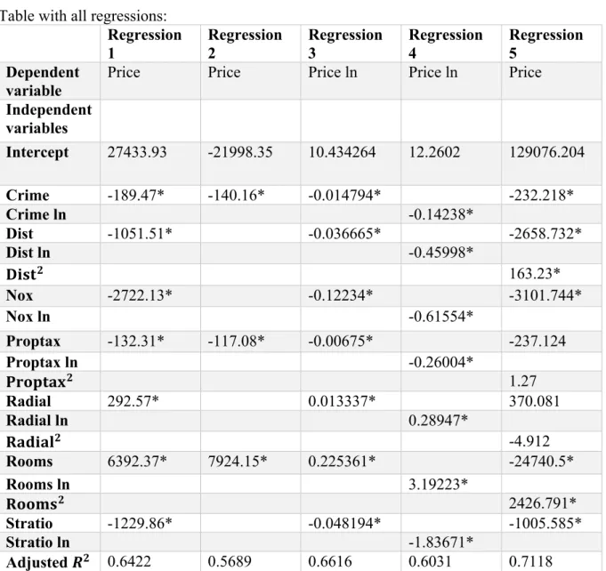
Table with all regressions:

Regression 1 Regression 2 Regression 3 Regression 4 Regression 5 Dependent variable

Price Price Price ln Price ln Price

Independent variables Intercept 27433.93 -21998.35 10.434264 12.2602 129076.204 Crime -189.47* -140.16* -0.014794* -232.218* Crime ln -0.14238* Dist -1051.51* -0.036665* -2658.732* Dist ln -0.45998* 𝐃𝐢𝐬𝐭𝟐 _163.23* Nox -2722.13* -0.12234* -3101.744* Nox ln -0.61554* Proptax -132.31* -117.08* -0.00675* -237.124 Proptax ln -0.26004* 𝐏𝐫𝐨𝐩𝐭𝐚𝐱𝟐 _1.27 Radial 292.57* 0.013337* 370.081 Radial ln 0.28947* 𝐑𝐚𝐝𝐢𝐚𝐥𝟐 _-4.912 Rooms 6392.37* 7924.15* 0.225361* -24740.5* Rooms ln 3.19223* 𝐑𝐨𝐨𝐦𝐬𝟐 _2426.791* Stratio -1229.86* -0.048194* -1005.585* Stratio ln -1.83671* Adjusted 𝑹𝟐_0.6422 _0.5689 _0.6616 _0.6031 _0.7118

All significant coefficients are market with (*).

Depending on the purpose of the study the number of independent variables can vary and sometimes including all the variables available is not the best choice. If they all are significant it is not necessary to exclude any variables from the regression.

As shown in the table above the adjusted 𝑅*_{increases with more variables included in the} regressions as Andersson, Jorner and Ågren (2007) explained regarding the 𝑅*_{. It is not} always the case with the adjusted 𝑅*_{, but it happened to occur in our regressions. Regression}

(30)

(5) has the highest adjusted 𝑅*_{and regression (2), with only three independent variables} showing the lowest adjusted 𝑅*_{. Only looking at the 𝑅}*_{get us to think that the regression (5)} is the best to select because it explain most of the variance of the dependent variable. This can be discussed since four of the independent variables where not significant. Therefore the highest 𝑅*_{is not always the most true or suitable regression.}

The interpretations for the variable nox can be made such as we can see that the variable always has a negative impact on the housing price even in logged form. As Rosen (1974) explained, the prices are determined both by internal and external factors. When looking at the variable nox we can see that the external factor environment has a negative impact on the price in all our equations. The variable nox shows that the environment has a big impact on the housing prices and that people care about where they are willing to live. To prove a strong connection between environment and housing price, as Wheeler (2012) and White (2010) talks about, would have been easier if we had access to more variables like accessibility to parks or lakes. Now we can only assume from looking at the variable nox that environment is important to people and there would probably been a strong relationship between similar variables explaining the environment and the housing price.

Looking at the variable radial shows that living near a highway increases the housing price, when the same variable is in log form it also has a positive effect on the price. When we look at the variable radial in squared form we can see that the total effect will still be positive when distance increases. This variable is not significant and cannot really be interpret but we made some comments on it since it is quite likely that this could be the case if it were significant. This depends most likely on the comfort of having a highway near by your house. Having too many highways does not increase the comfort instead you are living in a louder and noisier area. This is connecting to what Wheeler (2012) and White (2010) indicated in their research, that people feel better living near parks and green area. Consumers are not willing to pay as much for a house laying near several highways.

As Wheeler says, living near green area reduces stress and if your house is placed among several highways there is less space for parks and green area and maybe people would find it stressful to live in such a place. If we had more variables explaining the characteristics of living near a park or lake, we could compare this to highways and see what gives the highest

(31)

characteristics laying near a lake instead of a highway costs more money as Tyrväinen (1997) implies.

Going back to Lancaster’s (1966) example about the two cars in different colors it can be compared to the same house in two different neighborhoods, where crime is low in one of them and higher in the other one. The characteristics of the house are identical, the only difference is the location. It is shown in our regressions that crime always has a negative impact of the housing price and Sheppard (1997) has shown the connection how higher utility is leading to higher prices. By this it can be shown that it is the characteristics of the house that is yielding the utility, as Lancaster pointed out, otherwise the price would not have been reduced while crime is increasing.

The variable crime is what Rosen (1974) calls an external factor that influences the price. Referring back to the example, the two identical houses would yield different amounts of utility. Assuming consumers would want to maximize their utility, according to Pindyck and Rubinfeld (2013), they would choose the house where crime is lower since it is yielding more utility, at a given price. But for a consumer for whom the house with higher utility, comes with a higher housing price, they might maximize utility by ending up in the neighborhood where crime is decreasing housing prices.

According to Pindyck and Rubinfeld (2013) utility is based on preferences. The distance to employ centers is definitely something that varies in preference from a person to another. From the 5th_{regression, it appears like the distance has a negative effect on the housing price}

when increasing, until the distance reaches 8 miles. After 8 miles it seems like the increased distance instead becomes positive on the housing price. This might be the consumers who prefer to live on the countryside and therefore gain the most utility from living apart from any center.

As Samuelson (1955) explain a public good, such as the nature of the countryside, has the same possibility for anyone to consume it. But their preferences will determine if they will enjoy it and gain any utility by living close to it. The consumers who valuate living near their workplace are confirming what Tyrväinen (1997) implies about the hedonic pricing model. The housing prices are affected by aspects such as access to workplaces, this is also

(32)

confirmed by the regression. The short distance to the workplace brings comfort and yields utility to those who have certain preferences.

Sheppard (1997) explains how the price function is dependent of the characteristics of the house. Same goes for the utility. When the price of a house increases, the utility of owning a house will decrease. It is showed in a linear and a logarithmic regression that property tax always will have a negative effect on the housing price. For every additional $1000 increase, however, the total effect will still have a negative effect on the housing price. The variable proptax is not significant in regression (5) but we have made comments on the total effect. If the effect ever becomes positive it could depend on when property tax increases to a certain level, consumers with low income are already excluded from the market. The ones remaining on the market will be the medium/high income consumers for whom an increase in property tax may not affect the utility as much as for those with low income. This is a possible theory but since the variable is not significant we cannot make any interpretations about it.

Tyrväinen (1997) once again implies that housing prices are affected by the average number of rooms. In all linear regressions the variable rooms has a positive effect on the housing price, as predicted, because a higher price gives a greater housing area. When adding the variable rooms in quadratic form, the natural variable rooms become negative and the quadratic one becomes positive. The total effect from the two variables is negative until the average increases to 5 rooms, the 6th room will raise the housing price.

When adding the 6th _{room the house becomes more like a premium good and may be used for}

more purposes than just living in. For example, there is a room for a movie theatre, game room or other activities that may be considered as luxury.

Assuming the demand for the luxury houses is smaller compared to a regular house due to consumers preferences and mainly budget constraints. Even though the demand is smaller the price will be higher since all the characteristics are costly, also shown by the price function by Sheppard (1997). The characteristics bring a high status that may be considered worth paying for. The high status may be a reason for a consumer gaining utility from purchasing the house. Since we are on the subject status, it would have been interesting to have more variables to investigate it further. If buying a luxury house the expectations of the house are high and less

(33)

buying a cheaper house. Then you might have to select which of the internal or external factors are most preferable to still be able to buy a house within the budget constraint. Looking at the data that the regressions are based on, we find that the average number of rooms in the data collected is 9 rooms. This may be a reason why the 6th room is where the total effect becomes positive. The outcome might have been different if the data had been based on houses with up to 8 rooms. In the data there is a gap between 8 and 24 rooms. The data contains 132 observations that have 24 rooms in each house. On a total of 506

observations these 132 observations can give a mistaken idea about what the effect of each variable really is. The positive effect from the variable rooms might have been shown at a smaller number of rooms if we were to exclude the 132 observations. When excluding the 132 observations, the average number of rooms in the data falls to 4.44. By running a regression without the 132 observations might give a value of the effects that is closer to the truth. But because of time limitations, we chose not to do any more regressions.

The importance of environmental quality and how much extra money the consumers are willing to pay has been showed from Tyrväinen (1997). This is readable in the regression made. Since a worse school district will decrease the price, the importance of a good school is being displayed by the reduction in housing prices. Consumers with children may have this variable as a prioritized characteristic since most parents are concerned of the education for their children. A good school district may increase the demand for living in a certain area. A reason for this could be that the area becomes more popular to live in because the school is located nearby. Likewise if there were a worse school district the demand for living there would decrease which is readable from the regressions.

(34)

6. The result and conclusion

Here are the results and conclusion of the thesis presented

From analyzing all the regressions, we came to the conclusion that every characteristic has an effect on the price, this effect can either be positive or negative. Each characteristic provides a certain amount of utility to the consumer that is not gained by the house itself. Higher utility is causing higher housing prices. This confirms the idea behind the hedonic pricing model. The used data consists of mostly external variables, the effect of the internal variables has not been shown properly since we only had one internal variable available. It would have been interesting to see how the effect on the price from the internal variables differ from the external variables.

From the regressions made it is clear that the variables nox and rooms have the biggest effects on housing prices. From this we can come to the conclusion that environmental aspects are great influence on the housing price. The outcome of our study agrees that the two variables are a great influence, as previously demonstrated by studies used in this paper.

When buying a house one of the most important variables may be the number rooms. The impact of this variable in regression (5) was unexpected since the number of rooms had a negative effect until the fifth room then the effect became positive. Our expectations were that the price would increase for every additional room as it did in regression one to four. We believe that the result would have been different if we had more evenly distributed data. Every measured variable has an impact on the housing price but how big this impact is varies due to individual preferences which is decisive for the amount of utility gained. For example, being close to a highway may be highly valuated for some consumers while others prefer to live far away from highways and closer to different environmental aspects provided by the nature. Most of the effects from the variables matched our expectations while some of the variables are based on consumer´s preferences as explained above.

For future research in this field it would be beneficial to have more variables in the data set. Because it would allow us to get a greater understanding and make more profound analysis. In

(35)

our analysis we came across several theories that were not possible to test due to limited data, but would have been interesting to see the effects from.