Empirical analysis of unbalanced bidding on Swedish roads

(1)

Swedish National Road and Transport Research Institute www.vti.se

Empirical analysis of unbalanced bidding on Swedish roads

VTI Working Paper 2019:4

Johan Nyström

1,3

_{och Daniel Wikström}

2

1 _{Transport Economics, VTI, Swedish National Road and Transport Research Institute} 2_{Dalarna University}

Abstract

Based on anecdotal evidence, claims are made that unbalanced bidding is a major problem in the construction industry. This concept refers to a sealed price auction setting with asymmetric

information and unit prices, where information rents are extracted. Theoretical literature has shown that it is rational for an informed contractor to skew unit prices. However, empirical studies on the magnitude of the problem are lacking. As the first quantitative study based on European data, it is shown that unbalanced bidding exists, but in small magnitudes. The result is in line with earlier studies from the US.

Keywords

Unbalanced bidding, asymmetric information, information rent

JEL Codes

(2)

(3)

1

Empirical analysis of unbalanced bidding on Swedish roads

Johan Nyströma_{and Daniel Wikström}b

Abstract

Based on anecdotal evidence, claims are made that unbalanced bidding is a major problem in the construction industry. This concept refers to a sealed price auction setting with asymmetric information and unit prices, where information rents are extracted. Theoretical literature has shown that it is rational for an informed contractor to skew unit prices. However, empirical studies on the magnitude of the problem are lacking. As the first quantitative study based on European data, it is shown that unbalanced bidding exists, but in small magnitudes. The result is in line with earlier studies from the US.

Keywords: Unbalanced bidding, asymmetric information, information rent JEL codes: D22, D82, D86, H57, L47, L92

a_{Corresponding author. The Swedish National Road and Transport Research Institute, Department of}

Transport Economics, Box 55685, 102 15 Stockholm, Sweden (johan.nystrom@vti.se),

b _{Dalarna University Box 920 / 781 29 Borlänge (dwi@du.se)}

(4)

2

1.0 Introduction

Transport infrastructure is often defined as a public good and therefore provided by a public

entity. There are three ways for the government to undertake this responsibility. It can use

in-house personnel, public procurement to buy the service from the market or let private

contractors finance and take responsibility for providing infrastructure using a long-term

agreement (i.e. Public Private Partnerships, PPP). Which setting to use has been approached

theoretically by Hart et al. (1997) and Shleifer (1998), but the empirical answers are ambiguous

(see e.g. Jensen and Stonecash, 2005; Alonso et al., 2015; Hensher, 2015; Odolinski and Smith,

2016). This paper focuses on the public procurement setting (see e.g. Spagnolo, 2012; Tadelis,

2012), where a first-price sealed-bid auction is common when the government is providing

transport infrastructure (Gupta, 2001).

Incomplete contract theory (Grossman and Hart, 1986; Hart and Moore, 1989) has shown

that first-best contracts are hard to achieve. Asymmetric information enables informed bidders

to extract information rents through strategic pricing. Such strategies include predatory pricing

(Baumol, 2003), ex post renegotiations via the hold-up problem (Goldberg, 1976), quality

shading (Hart et al. 1997) and unbalanced bidding (Stark, 1974).

Unbalanced bidding is a potential pitfall when the public client uses unit price contracting

(UPC). If present, this is manifested by the client paying too much for the final product.

Unbalanced bidding comes from the contractor being better informed than the client (i.e.

asymmetric information), which the former uses to their advantage.

The concept is usually portrayed as a major problem of the construction industry. Experts often claim that “this is how it is done in the industry”. This perception is based on anecdotal evidence. Most of the academic papers are theoretical, showing that it is rational for an informed

contractor to use unbalanced bidding. However, there is a lack of empirical studies supporting

(5)

3

This paper sets out to empirically examine the problem of unbalanced bidding. A database

of 15 Swedish road projects with 2 772 unique item observations is used to approach the theory.

This is the first study, to our knowledge, to use a statistical approach on European data.

The paper starts by introducing the concept of unbalanced bidding, and follows this with a

description of research on the topic. Section 4 describes the data, after which the model is

introduced. The results are presented in section 6, followed by a robustness check of the

marginal cost proxy and the conclusions.

2.0 The concept of unbalanced bidding

The usual way for public clients to procure infrastructure is to use a unit price contact (UPC).

With such a contract, the client prepares and takes juridical responsible for the design.

Competitive bids from contractors are unit price vectors, related to a bill of quantities stipulated

by the client. The vector product of prices and quantities makes up the total price –often the

lowest price. Although this way of procuring is transparent and simple, it also permits strategic

behaviour that results in non-efficient equilibriums. Apart from the client setting the quantities

in a strategic manner (Mandell and Brunes, 2014), a more evident problem is the contractors

behaving strategically in the bidding process: i.e. unbalanced bidding.

There are two types of unbalanced bidding discussed in the literature; “front/back loading”

and error exploitation. A prerequisite for both types is the bidder being better informed than the

client. Front loading suggests that the contractors mark up unit prices on quantities that are

scheduled for early completion, trading off quantities for late completion (Arditi and

Chotibhongs, 2009; Skitmore and Cattell, 2011). Error exploitation involves the contractor

using misestimation in the client’s bill of quantities by raising unit prices on underestimated

(6)

4

bidding of the latter type. An example from road construction can be used to describe this type

of unbalanced bidding.

Assume that there are two inputs to building a road, provision of gravel and pavement. The

ex ante bill of quantities for the project estimates 100 m3 of gravel and 150 m2 of pavement. Assume that the contractors differ with regard to costs and information, where Contractor 2 has

a higher marginal cost on both inputs in comparison to Contractor 1. However, Contractor 2

also has private information, which Contractor 1 does not. Contractor 1 bids her marginal cost

at unit prices of 10. Contractor 2 can then use her superior information regarding the ex post

quantities and skew unit prices accordingly. As depicted in Table 1, Contractor 2 submits the

lower total bid and wins the contract.

Table 1 Ex ante bill of quantities and bids

Ex ante Bill of quantities Contractor 1’s bid (uninformed) Contractor 2’s bid (informed) Provision of gravel 100 m3 ₁₀ ₁₂ Pavement 150 m3 ₁₀ _8,5 Total bid 2 500 2475

The project starts and Contractor 2’s prediction – i.e. that the quantities of gravel will increase and pavement decrease – turns out to be correct. As seen in Table 2, Contractor 2’s

skewing of prices, based on her expectation of changing quantities, enables her to win the

contract and earn higher revenue.

Table 2 Contractor 2 submits the lower total bid and wins the contract

Ex post Actual quantities Contractor 1’s bid (uninformed) Contractor 2’s bid (informed) Provision of gravel 110 m3 ₁₀ ₁₂ Pavement 145 m3 ₁₀ _8,5

Final cost for the client 2 550 2553

Due to unbalanced bidding, the most efficient contractor does not win the contract and the

(7)

5

However, assuming that the contractor is risk neutral, the optimal way of skewing the bid

is to hand in zero-unit prices on the most overestimated quantity and maximise the unit prise

on the most underestimated quantity, as in Table 3.

Table 3 Contractor 2 being risk neutral

Ex ante Actual quantities Contractor 1’s bid (uninformed) Contractor 2’s bid (informed) Provision of gravel 110 m3 ₁₀ ₂₅ Pavement 145 m3 ₁₀ ₀

Final cost for the client 2 500 2 750

Such bidding behaviour would maximise the ex post profit.

3.0 Research on unbalanced bidding

The earliest papers on unbalanced bidding include Gates (1967) and Starks (1974), who

conceptualised the concept. Since then, two types of model regarding unbalanced bidding have

evolved. The first group of models aims at providing practical guidance for clients to detect

(Arditi and Chotibhongs 2009) and contractors to optimise (Cattell et al. 2010; Cattell et al.

2008; Yizhe and Youjie 1992) unbalanced bidding. These are practical models intended to help

practitioners.

The second type of model is directed at a theoretical audience and concerns market

efficiency. These are models typically found in economics, trying to predict bidding behaviour

and socio-economic efficiency. The two most prominent models were developed by Athey and

Levin (2001) and Ewerhart and Fieseler (2003). Both models are based on asymmetric

information between client and contractor and on risk-neutral contractors and result in corner

solutions. This refers to a situation in equilibrium where the contractors hand in zero-unit prices

for all quantities but the one that will increase the most, the most underestimated quantity (i.e.

the example shown in Table 3). Mandell and Nyström (2013) introduced risk aversion to this

(8)

6

Hence, there are rational arguments for an informed contractor to skew the bid. This is not

the same as the contractors actually doing it.

There are two empirical studies that look at evidence of unbalanced bidding. Both use data

from road construction in the US. Although not the focus of the paper, Bajari et al. (2014) show

that a 10 per cent quantity overrun will raise the corresponding unit price 0.5 per cent, which

they conclude is a modest amount. De Silva et al. (2015), using data from road construction in

Texas, US, do not find any correlation between deviations in quantities and prices.

The following sections will present an analysis looking at whether unbalanced bidding is

present in Sweden.

4.0 Data

The data for this study are gathered from the Swedish Transport Administration (Trafikverket).

It is based on 15 road construction projects procured by Trafikverket between 2006 and 2010.

All projects are road investments, geographically spread across Sweden. Each project is made

up of, on average, 186 ex ante specified quantities (items). These are estimated quantities by

the client of what it takes to build the specific road. Hence, data consists of 15 projects and 2

789 unique observations of quantities and unit prices.

Data has been collected in the form of so-called MSS files. These comprise a standardised

Excel sheet that all project leaders in Trafikverket use. The Excel sheet includes all quantities

used in a project, both estimated (ex ante) and final (ex post). Estimated quantities are defined

in different units; metres and square and cubic metres. The file also includes unit prices and

additional information such as project characteristics, additional orders and changes. There are

seven firms with winning bids in the data.

Following Bajari et al. (2014) and De Silva et al. (2015), the two main variables for

analysing unbalanced bidding is to relate changes in quantities to changes in prices. This is

(9)

7 100𝑝𝑖𝑘−𝑝̅𝑘

𝑝̅𝑘 , (1)

where pik is winning bidder i’s price for item k and 𝑝̅𝑘is the average winning bids across projects for item k. The average 𝑝̅𝑘, is an estimator of the ‘norm’ price of item k. Bajari et al. (2014) and De Silva et al. (2015) are using engineer estimates or Blue Book prices, but these are not

available in Sweden. Therefore, (1) is based on the winning bids in this data. This runs the risk

of producing a biased proxy of the marginal cost should all winning bidders skew their bids.

The engineer estimates and Blue Book prices are the same measure, but the risk of being biased

diminishes with more observations. A robustness check of the average price used are

undertaken in section 7.

Relative quantities are defined as the relative change between ex ante and ex

post quantities, expressed as:

100𝑞𝑖𝑘 𝑝

− 𝑞_𝑖𝑘𝑎 𝑞_𝑖𝑘𝑎 ,

(2)

where 𝑞_𝑖𝑘𝑎 is ex ante quantities and 𝑞_𝑖𝑘𝑝 ex post quantities.

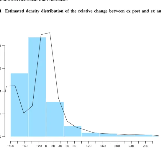
Table 4 presents summary statistics, showing that relative quantities can change quite

dramatically. The average change in quantities is 35.9 per cent but the most extreme increase

is over 12 000 per cent. Also note that some quantities specified in the UPCs were not used in

the production at all. Resulting in -100 per cent change. There are also large deviations in prices

(10)

8

Table 4 Summary statistics

N Mean St.

Dev. Min Max

Relative prices 2,788 -0 122.7 -100 3,363 Relative quantities 2,773 35.9 453.7 -100 12,307

Size of projects (1000 SEK) 15 42

384 43 039 1 528 132 663

Figure 1 gives a better picture of the whole distribution of relative quantities. For example,

more quantities decrease than increase.

Figure 1 Estimated density distribution of the relative change between ex post and ex ante quantities

Relative prices show a similar pattern, where some bids are much higher than the average

bid but the majority of bids are below the average bid (Figure 2).

−100 −60 −20 0 20 40 60 80 120 160 200 240 280 0.000 0.002 0.004 0.006 0.008 Realtive quantities (%) D e n s it y

(11)

9

Figure 2 Estimated density distribution of relative unit bids (prices)

The observed values of both variables show patterns that would be expected if bidders were

practising unbalanced bidding. Deviations of quantities in both directions enable profitable

skewing for an informed contractor. About 30 per cent of the quantities do not have any

deviation, while 28 per cent are over- and 42 per cent underestimated. Prices also show great

variation in both directions.

5.0 Empirical model

To examine the existence of unbalanced bidding in Sweden, this study follows Bajari et al.

(2014) and De Silva et al (2015). This is done by estimating the relationship between relative

unit bids with the difference in ex ante and ex post quantities. The following regression model

is used: 𝑌_𝑖𝑘 = 𝛼 + 𝛾𝑍_𝑖𝑘+ 𝜀_𝑖𝑘, (3) −100 −60 −20 0 20 40 60 80 120 160 200 240 280 0.000 0.002 0.004 0.006 0.008

Realtive unit bids (%)

D e n s it y

(12)

10

where 𝑌_𝑖𝑘 is the relative price for item k, given by the winning bidder i specified in eq. (1). The variable 𝑍𝑖𝑘is the relative quantities as defined by eq. (2).

The simple regression model in eq. (3) corresponds to the model used by Bajari et al. (2014)

and De Silva et al. (2015). Here, however, the dependent variable and the variable of interest

are expressed in percentage terms to simplify the interpretation. If the parameter 𝛾 is positive,

it indicates that bidders are skewing prices. Thus, quantity overrun implies overpricing and

underrun implies under-pricing. A more general specification is also used, where firm-specific

variables are included:

𝑌_𝑖𝑘 = 𝛼 + ∑ 𝛼_𝑔𝐷𝑔_𝑖 𝐺 𝑔=2 + 𝛾₁𝑍_𝑖𝑘+ ∑ 𝛾_𝑔𝐷𝑔_𝑖 × 𝑍_𝑖𝑘 𝐺 𝑔=2 + 𝜀_𝑖𝑘, (4)

Firm dummies, where 𝐷𝑔𝑖, equals one if g=i and zero otherwise, α is the intercept and εik is an error term. The effect of skewing for Firm 1, the reference firm, is γ1, for any other firm (g=2,…,G) the effect is γ1+γg. Hence, if γg>0, the firm g skews prices to a larger extent than the reference firm. If γ1=0, the reference-level firm does not skew prices.

As pointed out by both Bajari et al. (2014) and De Silva et al. (2015), the items of the same

project are very likely dependent, which also makes the errors dependent across project items.

Therefore, Bajari et al. (2014) and De Silva et al. (2015) make inferences based on

project-clustered standard errors. In their case this is rather straightforward, as the large number of

projects enables the asymptotic theory for standard errors. The issue becomes more complicated

with only 15 projects. Cameron et al. (2008) show that small-sample refinement can be achieved

through bootstrap-based methods, in particular the wild bootstrap method. When trying this

method with our data, it tends to break down. The few times it works, the same results as with

standard cluster inference with degrees of freedom correction for small samples are found, as

suggested by Cameron and Miller (2015). Therefore, the latter method is used throughout the

(13)

11

Bajari et al. (2014) and De Silva et al. (2015) also make estimations with item-code fixed

effects. De Silva et al. (2015) do not comment on the fixed effects and Bajari et al. (2014) justify this action only by allowing for “heteroskedasticity within an item code”. This paper has chosen not to include these fixed effects, as there is a potential problem of erasing any

between-item-code effects. If a firm expects a lower ex post quantity of one item and a higher ex post quantity

of a second item, then unit prices will be lowered and raised accordingly. If item fixed effects

are included, this between-item effect of skewing is erased. Nevertheless, versions both with

and without will be presented below, where the former will capture a potential between effect.

6.0 Results

In this section, the results from estimations of models in eq. (3) and eq. (4) are presented.

Estimations for the complete data material as well as for a subset consisting only of earthwork,

excavation and filling will be presented. Testing the subset of earthwork, excavation and filling

is based on anecdotal evidence that these parts of the contracts are especially exposed to

unbalanced bidding. The results for the complete data material are given in Table 6 and the

(14)

12

Table 5 Regression results

Dependent variable: r_p (1) (2) (3) r_q 0.0001 0.022*** _0.021*** (0.003) (0.003) (0.0002) Firm2 -0.309 (5.455) Firm3 27.470 (26.530) Firm4 3.405 (2.820) Firm5 -14.895*** (2.483) Firm6 -2.480 (17.380) Firm7 -30.317 (28.094) r_q:Firm2 -0.019*** _-0.021*** (0.006) (0.005) r_q:Firm3 0.177*** _0.159*** (0.008) (0.001) r_q:Firm4 -0.022*** _-0.022*** (0.004) (0.003) r_q:Firm5 0.003 0.007 (0.012) (0.005) r_q:Firm6 -0.025*** _-0.024*** (0.002) (0.002) r_q:Firm7 0.056 -0.017*** (0.070) (0.002) R2 0 0.007 0.013

(15)

13

Adjusted R2 0 0.003 0.007

Firm reference level: Firm 1

Observations 2,772 2,772 2,772

Note:

*_p<0.05,**_p<0.01,***_{p<0.001; standard errors in} parentheses

In line with Bajari et al. (2014) and De Silva et al. (2015), the R2 values are low when all

items are included, as seen in Table 5. The R2 values are higher for the subset regression (see

Table 6). This indicates that the firms pay extra attention to the subset codes. Table 5 does not

indicate unbalanced bidding to any larger extent, as seen in specification 1. However, allowing

for firm differences in skewing by including the interactions, then there are firms with

significant unbalanced bidding behaviour (specifications (2) and (3)).

Table 6 Regression results for excavation and filling

Dependent variable: r_p (1) (2) (3) Constant 0.129 20.251 12.841 (2.298) (12.292) (20.327) r_q -0.001 0.009 0.003 (0.003) (0.016) (0.015) Firm2 7.540 (16.823) Firm3 161.737*** (26.185) Firm4 -24.779* (11.620) Firm5 -50.793*** (14.821) Firm6 -22.871* (11.020) Firm7 -9.244

(16)

14 (21.440) r_q:Firm2 -0.012 -0.006 (0.038) (0.036) r_q:Firm3 0.690*** _1.114*** (0.165) (0.160) r_q:Firm4 -0.009 -0.002 (0.016) (0.016) r_q:Firm5 0.312* _0.073 (0.130) (0.149) r_q:Firm6 -0.012 -0.005 (0.016) (0.016) r_q:Firm7 0.041 -0.058 (0.061) (0.058)

Year dummies No Yes Yes

R2 0 0.096 0.217

Adjusted R2 -0.001 0.082 0.199

Observations 717 717 717

Note: *_p<0.05,**_p<0.01,***_{p<0.001; standard errors in parentheses}

Focusing on specification (3), Firm 1 (the reference level) skews quite moderately. When a

quantity changes ex post by 1 per cent then Firm 1, on average, increases prices by 0.021 per

cent according to the regression. For Firm 3, a 1 per cent ex post change gives about

(0.021+0.159=) 0.18 per cent increase in prices. Firm 5 is not significantly different from Firm

1, the reference firm. Firms 2, 4, 6 and 7 do not significantly skew at all. As an example, the

effect of relative quantities on prices is slightly negative for Firm 6, (0.021-0.024=-0.003), but

insignificant when the sum of the coefficients is tested. Reasons for why some firms are not

(17)

15

Furthermore, Firm 3 also stands out, with overall higher bids than other contractors – for

example, it has on average 66.7 per cent higher bids than Firm 1 according to regression (3) in

Table 6. Firm 7 has an even higher estimated value, but there is too much uncertainty attached

to this estimate – for example, the lower limit of the 95 per cent confidence interval is -83 per

cent. These large deviations in price may look unrealistically large, but, although all projects

are road projects, they may differ vastly in character. For example, building a tunnel is relatively

risky and should imply overall higher pricing compared to more standard projects.

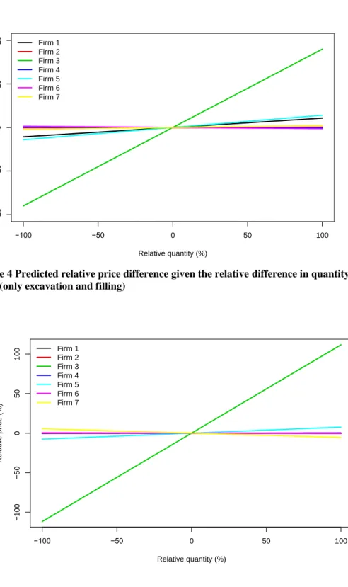
When looking at the results for the sub-sample of earthwork, excavation and filling, the

results change slightly. Firm 3 skews more, while there is no evidence that the other firms

unbalance at all on these activities. For Firm 3, if quantities increase by 1 per cent, prices are

on average 1.11 per cent higher.

Item-code fixed effects are also tested, resulting in lower R2-values decreases, indicating

that these effects are not relevant (see results in the Appendix).

The overall pricing on the subset of activities varies quite much across firms, as can be seen

in Table 6. For Firm 3, these quantities seem to be where information rents are made. On

average, they price these quantities 162 per cent higher than Firm 1. This may appear

unrealistically high but, as shown in Table 4, some quantities firms may be thousands of per

(18)

16

Figure 3 and 4 presents predicted relative difference in prices due to relative differences in

quantity. Figure 3 is for all items and Figure 4 for the sub-sample. Note that Firm 3 stands out

from the other firms.

Figure 3 Predicted relative price difference given the relative difference in quantity ex ante to ex post (per cent)

Figure 4 Predicted relative price difference given the relative difference in quantity ex ante to ex post (per cent) (only excavation and filling)

−100 −50 0 50 100 − 2 0 − 1 0 0 1 0 2 0 Relative quantity (%) R e la ti v e p ri c e ( % ) Firm 1 Firm 2 Firm 3 Firm 4 Firm 5 Firm 6 Firm 7 −100 −50 0 50 100 − 1 0 0 − 5 0 0 5 0 1 0 0 Relative quantity (%) R e la ti v e p ri c e ( % ) Firm 1 Firm 2 Firm 3 Firm 4 Firm 5 Firm 6 Firm 7

(19)

17

Firm 3 can also be used as an example of the information rent in a specific project by

applying the estimates. This gives an ex ante bid of 136 995 euro and the ex post cost of 145

915 euro, amounting to an information rent of 8 920 euro.

7.0 Robustness check

In order to check the potential problem of biased average unit prices, this section replaces the

average winning unit prices with prices from another database on reinvestments of highways in

Sweden (see Table 7). The only difference from the previous analysis is that relative prices are

calculated with different average prices. However, since not all items of the investment projects

existed for the reinvestments projects, the sample size decreases by about 50 per cent.

Table 7 Regression results

Dependent variable: r_p2 (1) (2) (3) r_q -0.001 0.027** _0.035*** (0.006) (0.009) (0.000) Firm2 -4.073 (6.641) Firm3 5.521 (19.848) Firm4 -12.334 (8.110) Firm5 46.156* (21.104) Firm6 42.640 (52.773) Firm7 -97.463*** (22.001) r_q:Firm2 -0.126*** _-0.140***

(20)

18 (0.038) (0.037) r_q:Firm3 0.478*** _0.398*** (0.032) (0.0004) r_q:Firm4 -0.028* _-0.032*** (0.012) (0.010) r_q:Firm5 0.151 0.123 (0.119) (0.112) r_q:Firm6 -0.031*** _-0.041*** (0.008) (0.008) r_q:Firm7 0.105* _0.038*** (0.053) (0.001) R2 0 0.012 0.018 Adjusted R2 -0.001 0.004 0.006

Note:

The results when applying different estimates of unit prices are similar to the main

specification (see eq.1). However, Firm 3 seems to unbalance even stronger (compared to Table

5). This is expected if the averages used in the original analysis are biased. As discussed earlier,

if all firms skew the same unit prices, there will a bias towards zero – that is, relative prices

look unbalanced. The interaction term for Firm 2 in Table 8 indicates a negative skew, which

has no logical bearing in theory. This is regarded as a peculiarity of the sample that remains

when applying prices from the projects.

Table 8 Regression results for excavation and filling

Dependent variable:

r_p2

(1) (2) (3)

(21)

19 (0.008) (0.982) (0.940) Firm2 -14.116 (54.384) Firm3 144.321* (71.709) Firm4 -65.942 (36.567) Firm5 -103.580* (41.483) Firm6 -85.941* (33.981) Firm7 -100.748 (64.155) r_q:Firm2 -0.165 -0.499 (0.985) (0.942) r_q:Firm3 2.869** _2.781** (1.041) (0.995) r_q:Firm4 -0.129 -0.463 (0.982) (0.940) r_q:Firm5 0.595 0.048 (1.065) (1.034) r_q:Firm6 -0.130 -0.461 (0.982) (0.940) r_q:Firm7 -0.065 -0.445 (0.991) (0.948)

R2 0 0.228 0.32

Adjusted R2 -0.003 0.202 0.285

Note:

(22)

20

The results for the subset of activities in Table 8 makes the original results even stronger.

No firm, apart from Firm 3, skews prices systematically. The biggest difference to the original

results is the magnitude of the skewing of Firm 3, which has doubled. This again is what might

be expected if the averages used in the original results are biased. Another explanation could

be that the sample of activities shrinks because not all activities in the original analysis existed

in the reinvestment projects. In this case the remaining activities would be a subsample that

Firm 3 exploits for skewing.

8.0 Conclusion

There is a consensus among experts in the construction industry that unbalanced bidding is a

huge problem. This is based on anecdotal evidence, with no solid empirical foundation. Apart

from the inefficiency perspective, there is often a moral argument against unbalanced bidding.

Contractors taking advantage of their superior information and substandard UPCs are portrayed

as immoral. But if a contractor were not to skew in a rational manner, they would be called to

account by the shareholders of the company for not maximising profit. Hence, the moral

argument is not valid.

However, there is little point in discussing the problem of unbalanced bidding unless one

knows the extent of the issue. This first quantitative study using European data confirms the

results of earlier American studies: unbalanced bidding is not a major issue.

This study shows that unbalanced bidding exists in the Swedish road construction market.

However, despite its portrayal in the debate it is not a widespread phenomenon. Although

several firms skew their bids, the magnitude of the skew is small.

One firm stands out from the rest. When making the analysis on all items, this firm increases

prices by on average 0.16 per cent when quantities are anticipated to increase by 1 per cent.

(23)

21

anticipated increase of quantities of 1 per cent entails a 1.11 per cent increase in unit prices.

(24)

22

References

Alonso, J. M., Clifton, J., & Díaz-Fuentes, D. (2015). Did new public management matter? An

empirical analysis of the outsourcing and decentralization effects on public sector size.

Public Management Review, 17, 643–660.

Arditi, D., & Chotibhongs, R. (2009). Detection and prevention of unbalanced bids.

Construction Management & Economics, 27, 721–732.

Athey, S., & Levin, J. (2001). Information and competition in U.S. Forest Service timber

auctions. Journal of Political Economy, 109, 375–417.

Bajari, P., Houghton, S., and Tadelis, S. (2014). Bidding for incomplete contracts: An empirical

analysis of adaptation costs. American Economic Review, 104, 1288–1319.

Baumol, W.J (2003). Principles relevant to predatory pricing. In Hope, E. (ed.), The Pros and

Cons of Low Prices (pp. 15–37), Stockholm: Konkurrensverket.

Cameron, C., Gelbach, B. & Miller, D. (2008). Bootstrap-based improvements for inference

with clustered errors. The Review of Economics and Statistics, 90 (3), 414–427.

Cameron, C. & Miller, D. (2015) A practitioner's guide to cluster-robust inference. Journal of

Human Resources, 50 (2), 317–373.

Cattell, D.W., Bowen, P.A., & Kaka, A.P. (2008). A simplified unbalanced bidding model.

Construction Management & Economics, 26, 1283–1290.

Cattell, D.W., Bowen, P.A. & Kaka, A.P. (2010). The risks of unbalanced bidding. Construction

Management & Economics, 28, 333–344.

De Silva, D., Dunne, T., Kosmopoulou, G. & Lamarche C. (2015). Project modifications and

bidding in highway procurement auctions. Federal Reserve Bank of Atlanta, Working Paper

2015-14. December.

Ewerhart, C., & Fieseler, K. (2003). Procurement auctions and unit-price contracts. Rand

(25)

23

Gates, M. (1967). Bidding strategies and probabilities. Journal of the Construction Division,

93, 75–107.

Goldberg, V.P. (1976). Regulation and administered contracts. The Bell Journal of Economics,

7, 426–448.

Grossman, S & Hart, O. (1986). The costs and benefits of ownership: A theory of vertical and

lateral Iitegration. Journal of Political Economy, 94, 691–719.

Gupta, S. (2001). The effect of bid-rigging on prices: A study of the highway construction

industry. Review of Industrial Organization, 19, 453–467.

Hart, O., Moore, J. (1990). Property rights and the nature of the firm. Journal of Political

Economy, 98, 1119–1158.

Hart, O., Shleifer, A., Vishny, R. (1997). The proper scope of government: Theory and an

application to prisons. Quarterly Journal of Economics, 112, 1127–1161.

Hensher, D. (2015). Cost efficiency under negotiated performance-based contracts and

benchmarking. Journal of Transport Economics and Policy, 49(1), 133–148.

Jensen, P., & Stonecash R (2005). Incentives and the efficiency of public sector-outsourcing

contracts. Journal of Economic Surveys, 19, 767–787.

Mandell, S. and Brunes, F. (2014) Quantity choice in unit price contract procurements. Journal

of Transport Economics and Policy, 48(3), 483–497

Mandell, S., Nyström, J. (2013). Too much balance in unbalanced bidding. Studies in

Microeconomics, 1, 23–35.

Odolinski,K., Smith. A (2016) Assessing the cost impact of competitive tendering in rail

infrastructure maintenance services: Evidence from the Swedish reforms (1999 to 2011),

Journal of Transport Economics and Policy, 50 (1), 93–112.

Shleifer, A (1998). State versus private ownership. Journal of Economic Perspectives, 12, 133–

(26)

24

Spagnolo, G (2012). Reputation, Competition and Entry in Procurement.” International Journal

of Industrial Organization, 30, 291–296

Stark, R. (1974). Unbalanced highway contract tendering. Operational Research Quarterly 25,

373–388.

Tadelis, S. (2012). “Public Procurement Design: Lessons from the Private Sector.”

International Journal of Industrial Organization, 30(3): 297-302.

Yizhe, T., Youjie, L. (1992). Unbalanced bidding on contracts with variation trends in client-

(27)

25

Appendix

Fixed effects estimations

Tabel 9 Fixed effects estimation on the complete data material

Dependent variable: r_p (1) (2) (3) r_q 0.0001 0.024*** _0.022*** (0.003) (0.004) (0.004) Firm2 -1.808 (11.991) Firm3 33.110 (40.495) Firm4 2.187 (7.554) Firm5 -18.394* (8.944) Firm6 -4.692 (17.649) Firm7 -43.732 (42.496) r_q:Firm2 -0.022** _-0.021* (0.007) (0.009) r_q:Firm3 0.180*** _0.153*** (0.016) (0.013) r_q:Firm4 -0.024*** _-0.023*** (0.005) (0.005) r_q:Firm5 0.005 0.014 (0.017) (0.013) r_q:Firm6 -0.027*** _-0.025*** (0.004) (0.005) r_q:Firm7 0.049 -0.017

(28)

26

(0.083) (0.021)

Item-code fixed effects Yes Yes Yes

R2 0 0.009 0.017

Adjusted R2 -0.128 -0.123 -0.117

Note:

Tabel 10 Fixed effects results when only codes that start with “CB” or ”CE” are included

Dependent variable: r_p (1) (2) (3) r_q -0.002* _0.010*** _0.001 (0.001) (0.001) (0.001) Firm2 7.795 (4.332) Firm3 163.261*** (8.253) Firm4 -35.833*** (5.958) Firm5 -58.274*** (6.161) Firm6 -31.783*** (5.400) Firm7 -14.670 (8.156) r_q:Firm2 -0.017* _-0.009 (0.007) (0.008) r_q:Firm3 0.733*** _1.142***

(29)

27 (0.163) (0.019) r_q:Firm4 -0.010*** _-0.0005 (0.001) (0.001) r_q:Firm5 0.482*** _0.268*** (0.045) (0.032) r_q:Firm6 -0.011*** _-0.003* (0.001) (0.001) r_q:Firm7 0.044*** _-0.043*** (0.011) (0.004)

Item-code fixed effects Yes Yes Yes

R2 0 0.117 0.245

Adjusted R2 -0.16 -0.041 0.102

Note: