Locally Induced Predictive Models
Ulf Johansson, Tuve Löfström, Cecilia Sönströd School of Business and Informatics
University of Borås Borås, Sweden
{ulf.johansson, tuve.lofstrom, cecilia.sonstrod}@hb.se
Abstract—Most predictive modeling techniques utilize all avail-able data to build global models. This is despite the well-known fact that for many problems, the targeted relationship varies greatly over the input space, thus suggesting that localized models may improve predictive performance. In this paper, we suggest and evaluate a technique inducing one predictive model for each test instance, using only neighboring instances. In the experimentation, several different variations of the suggested algorithm producing localized decision trees and neural network models are evaluated on 30 UCI data sets. The main result is that the suggested approach generally yields better predictive performance than global models built using all available training data. As a matter of fact, all techniques producing J48 trees obtained significantly higher accuracy and AUC, compared to the global J48 model. For RBF network models, with their inherent ability to use localized information, the suggested approach was only successful with regard to accuracy, while global RBF models had a better ranking ability, as seen by their generally higher AUCs.
Index Terms—Local learning, Predictive modeling, Decision trees, RBF networks
I. INTRODUCTION
Exploiting available data in order to extract useful and actionable information is the overall goal of the generic activity termed data mining. Some data mining techniques directly obtain the information by performing a descriptive partitioning of the data. More often, however, data mining techniques utilize stored data in order to build predictive models.
Predictive modeling combines techniques from several dis-ciplines. Many algorithms and techniques come from machine
learning, i.e., the sub-field of artificial intelligence focused on programs capable of learning. In the data mining context, learning most often consists of obtaining a (general) model from examples, i.e., data instances where the value of the target variable is known. Since the purpose of all predictive modeling is to apply the model on novel data (a test or production set), it is absolutely vital that the model generalizes well to unseen data. More precisely, for predictive classification, the number of incorrect classifications (the error rate) should be minimized - or the number of correct classifications (the accuracy) should be maximized.
As described above, predictive modeling normally consists of a two-step process: first an inductive step, where the model is constructed from the data, and then a second, deductive, step where the model is applied to the test instances. An alternative approach is, however, to omit the model building entirely and directly classify novel instances based on available training
instances. Such approaches are called lazy learners or instance
based learners. The most common lazy approach is nearest
neighbor classification, which classifies a test instance based on the majority class among the k closest (according to some distance measure) training instances. The value k is a parameter to the algorithm, and the entire technique is known as k-Nearest
Neighbor (kNN). kNN, consequently, does not, in contrast to techniques like neural networks and decision trees, use a global model covering the entire input space. Instead, classification is based on local information only.
Model building is clearly data-driven, making the validity of the process dependent on some basic, although most often not explicitly expressed, assumptions. Most importantly, the instances used for the actual training of the model must be good examples to learn from. Despite this, most techniques simply use all available instances for model training, thus prioritizing the global aspects of the model, while possibly ignoring important local relationships. In this paper, we apply the localized aspect of instance based learning to predictive modeling. More specifically, we evaluate different algorithms building localized decision tree and neural network models by using only a subset of the available training data. The main idea suggested here is to use neighboring instances to build one model for each test instance.
II. BACKGROUND
A predictive classification model is a function f mapping each instance x to one label in a predefined set of discrete classes {c1, c2, . . . , cn}. Normally, predictive models are
ob-tained by applying some supervised learning technique on historical (training) data. Most supervised learning techniques require that values for the target variable are available for all training instances, i.e., the training instances must be labeled. A training instance, thus, consists of an input vector x(i) with a corresponding target value y(i). The predictive model is an estimation of the function y= f (x; θ) able to predict a value y, given an input vector of measured values x and a set of estimated parameters θ for the model f . The process of finding the best θ values is the core of the learning technique.
The use of neighboring instances for the actual classi-fication makes it, in theory, possible for kNN to produce arbitrarily shaped decision boundaries, while decision trees and rule-based learners are constrained to rectilinear decision boundaries. Standard kNN is a straightforward classification technique that normally performs quite well, in spite of its
simplicity. Often, standard kNN is used as a first choice just to obtain a lower bound estimation of the accuracy that should be achieved by more powerful methods see e.g., [1]. Unfortunately, standard kNN is extremely dependent on the parameter value k. If k is too small, the algorithm becomes very susceptible to noise. If k is too large, the locality aspect becomes less important, typically leading to test instances being misclassified based on training instances quite different from the test instance.
A. Related work
Applying lazy techniques to prediction has been studied both for regression, such as in Quantitative Structure-Activity Relationship (QSAR) modeling in the medicinal chemistry domain [2], [3], and for classification [4], [5], [6], [7]. In the QSAR modeling, the motivation for the local approach is the assumption that similar compounds have similar biological activities, as studied in [8]. One of the first local approaches in QSAR modeling was suggested in [3], where a locally weighted linear regression was utilized in the analysis. In [2], the local regression approach is evaluated and contrasted to the global approach using random forests, support vector machines, and partial least squares models on both simulated and real world data. The results show that the local approach has a relatively high computational cost, high risk in defining locality and no reliable increase in predictive performance, indicating that the local approach might not be very successful for regression in general and for QSAR modeling in particular. For classification, a number of local approaches have been proposed. Friedman proposed the lazy decision tree algorithm, which builds a decision path for each test instance instead of a global decision tree [9]. The lazy decision tree algorithm has also been utilized in boosted ensembles [4]. A similar approach was employed to build bagged ensembles in [5], with the difference that the trees used were lazy option trees [10]. An option tree is a decision tree in which a given internal node in the tree is split in multiple ways (using multiple attribute-value tests, or “options”). The final probability estimate is the average of the estimates produced by each of these options. In [7], a local approach is used to build a global decision tree where lazy trees for each test instance are built in each leaf. The aim of this global lazy tree is to achieve good ranking capability. All these approaches build a model for each test instance using the complete training set.
A bagging approach for very weak classifiers, which utilizes a local approach similar to the one presented in this paper, can be found in [6]. The algorithm trains an ensemble of bagged very weak models, such as decision stumps, based on locally selected instances. The differences to our approach lies both in the kind of model being built and in how the selection of the nearest neighbors is performed.
III. METHOD
As described in the introduction, the overall purpose is to evaluate the effect of using neighboring instances to train one
model for each test instance. In particular, we compare the pre-dictive performance of this approach to the standard approach, i.e., using all available data to build one, global, model. For simplicity, and to allow easy replication of the experiments, the Weka workbench [11] is used for the experimentation. For the actual modeling, we elected to use one decision tree technique and one neural network technique. More specifically, the Weka implementation of C4.5 [12] called J48, and the radial basis function network (RBF) as implemented in Weka were used. During experimentation, all Weka parameter settings were left at the default values.
It must be noted that J48 trees and RBF networks have some fundamentally different properties which are of importance for this study. More specifically, the J48 technique does not, in any way, explicitly utilize any concepts related to proximity in the attribute space. An RBF network, on the other hand, when trained for classification, first uses the k-means clustering algorithm to provide the basis functions and then learns a logistic regression on top of that. So, simply put, even a standard RBF network trained using all available data is trained to utilize at least some of the locality aspect of the data set. With this in mind, it is quite interesting to compare the results for the two techniques, when used for producing locally trained models.
This study contains two experiments. In the first experiment, the suggested approach is tested by using different percentages of the available training data for model building. Altogether five different fractions are evaluated; 1%, 10%, 25%, 50%, and100%. So, as an example, when 10% is used for training J48 models, this means that for each test instance, one J48 tree is built using the 10% closest instances, to classify just that instance. For all distance calculations, the standard method used for lazy learners in Weka is applied.
In the second experiment, we test two algorithms aimed at automatically selecting, for each test instance, a suitable fraction of the training instances for the model building. This is, of course, similar to finding an appropriate value for the parameter k in kNN. The first algorithm uses standard internal cross-validation to select the percentage of instances to use. For this, the Weka meta technique CVParameter Selection, utiliz-ing ten internal folds was used. For simplicity, the fractions available to choose from were the same as in Experiment, i.e., 1%, 10%, 25%, 50%, and 100%. It must be noted that this selection is performed once per fold, not once per instance.
The second algorithm employs the machine learning tech-nique used to build the model (i.e. J48 or RBF) to find the appropriate k-value using both the evaluated test instance and the nearest neighbors used for training. A model is built using the k nearest neighbors from the training set for each
k-value between the number of classes +1 up to an upper limit. The upper limits tested were 10% and 25% of all instances available. To select which of the local models to use, a probability distribution over the classes is achieved by evaluating the model on the nearest neighbors and the test instance. The model achieving the most certain prediction on any class is selected as the model to use. The probabilities are
adjusted using Laplace to account for the greater uncertainty when estimating the probabilities on smaller samples, i.e. when
kis smaller. For simplicity, these two versions of the algorithm are referred to as A10 and A25.
For the evaluation, predictive performance is measured using both accuracy and area-under-the-ROC-curve (AUC). While accuracy is based only on the classifications, AUC measures the ability to rank instances according to how likely they are to belong to a certain class; see e.g., [13]. AUC can be interpreted as the probability of ranking a true positive instance ahead of a false positive; see [14]. Since 10x10-fold cross-validation was used, all reported performance measures are averaged over the 100 folds. The 30 data sets used are all publicly available from the UCI Repository [15].
IV. RESULTS
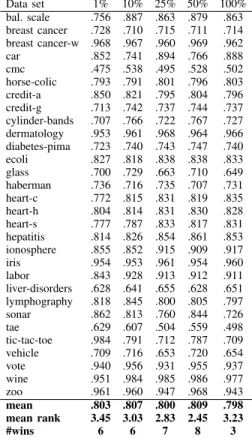
Table I below shows accuracy results for J48. One first, important, observation is that the results vary greatly between the data sets. A closer inspection shows that no specific training size is always superior to any other training size. As a matter of fact, all training fractions evaluated obtain the highest accuracy on at least two data sets. In addition, on most data sets, there is no clear trend; i.e., the pattern is neither the less data used the
higher accuracynor the more data used the higher accuracy.
TABLE I
EXP. 1: LOCALLY TRAINEDJ48MODELS. ACCURACY FOR DIFFERENT TRAINING SIZES
Data set 1% 10% 25% 50% 100% bal. scale .862 .695 .795 .793 .778 breast cancer .740 .717 .677 .681 .743 breast cancer-w .969 .961 .967 .967 .950 car .898 .924 .935 .933 .922 cmc .485 .509 .503 .501 .514 horse-colic .810 .837 .826 .836 .852 credit-a .856 .848 .847 .844 .856 credit-g .709 .713 .735 .733 .712 cylinder-bands .724 .694 .682 .704 .578 dermatology .964 .963 .964 .963 .941 diabetes-pima .716 .728 .753 .746 .745 ecoli .844 .824 .845 .838 .828 glass .700 .714 .746 .757 .676 haberman .735 .730 .664 .664 .722 heart-c .772 .801 .801 .791 .771 heart-h .804 .787 .804 .789 .802 heart-s .777 .787 .791 .784 .782 hepatitis .814 .807 .822 .821 .792 ionosphere .860 .858 .913 .925 .897 iris .954 .951 .935 .949 .947 labor .843 .894 .913 .884 .786 liver-disorders .626 .622 .646 .662 .658 lymphography .817 .831 .797 .815 .758 sonar .862 .772 .800 .803 .736 tae .629 .536 .517 .545 .574 tic-tac-toe .976 .957 .953 .931 .853 vehicle .706 .731 .747 .751 .723 vote .942 .966 .963 .962 .966 wine .951 .961 .979 .971 .932 zoo .961 .943 .935 .919 .926 mean .810 .802 .808 .809 .791 mean rank 2.90 3.10 2.50 2.83 3.67 #wins 10 2 11 4 3
On the other hand, when looking at overall mean accuracies
and ranks, it is obvious that the standard approach (using all available data to build one global model) is clearly the worst. Comparing the different training sizes, using the smallest training set (1%), i.e., for some data sets only a handful of instances, is remarkably often the best choice. Somewhat surprisingly, training using only1% actually obtained the high-est mean accuracy overall. Comparing mean ranks, however, both 25% and 50%, obtained slightly better results than 1%. To determine statistically significant differences, we compare mean ranks and use the statistical tests recommended by Demšar [16] for comparing several classifiers over a number of data sets, i.e., a Friedman test [17], followed by a Bonferroni-Dunn post-hoc test [18]. With five classifiers, 30 data sets and treating the standard approach (training one global model using all data) as the control, the critical distance (for α = 0.05) is 0.91. So based on these tests, training one model per test instance using the25% closest instances produced significantly more accurate models than the standard approach.
Table II below shows accuracy results for the RBF net-works.
TABLE II
EXP. 1: LOCALLY TRAINEDRBFMODELS. ACCURACY FOR DIFFERENT TRAINING SIZES
Data set 1% 10% 25% 50% 100% bal. scale .756 .887 .863 .879 .863 breast cancer .728 .710 .715 .711 .714 breast cancer-w .968 .967 .960 .969 .962 car .852 .741 .894 .766 .888 cmc .475 .538 .495 .528 .502 horse-colic .793 .791 .801 .796 .803 credit-a .850 .821 .795 .804 .796 credit-g .713 .742 .737 .744 .737 cylinder-bands .707 .766 .722 .767 .727 dermatology .953 .961 .968 .964 .966 diabetes-pima .723 .740 .743 .747 .740 ecoli .827 .818 .838 .838 .833 glass .700 .729 .663 .710 .649 haberman .736 .716 .735 .707 .731 heart-c .772 .815 .831 .819 .835 heart-h .804 .814 .831 .830 .828 heart-s .777 .787 .833 .817 .831 hepatitis .814 .826 .854 .861 .853 ionosphere .855 .852 .915 .909 .917 iris .954 .953 .961 .954 .960 labor .843 .928 .913 .912 .911 liver-disorders .628 .641 .655 .628 .651 lymphography .818 .845 .800 .805 .797 sonar .862 .813 .760 .844 .726 tae .629 .607 .504 .559 .498 tic-tac-toe .984 .791 .712 .787 .709 vehicle .709 .716 .653 .720 .654 vote .940 .956 .931 .955 .937 wine .951 .984 .985 .986 .977 zoo .961 .960 .947 .968 .943 mean .803 .807 .800 .809 .798 mean rank 3.45 3.03 2.83 2.45 3.23 #wins 6 6 7 8 3
Here, too, it is obvious that the standard approach most often results in weaker models than the locally trained models. Looking at the mean accuracy over all data sets, all options using locally trained models outperform the standard approach. All in all, however, considering the mean ranks and using the
statistical tests described above, the standard approach is not significantly worse than any of the locally trained versions.
Comparing these results to the J48 results, the main dif-ference is that here it seems better to use more data; i.e., the best results overall are obtained using50%, while using only 1% is the worst option. Still, the results vary considerably over the different data sets, even if the mean accuracies are quite similar. Specifically, the number of wins are very evenly distributed between the different training fractions.
The AUC results for J48 models are presented in Table III below. Regarding AUC, the picture is actually quite clear. Somewhat unexpectedly, all locally trained models clearly outperform the standard approach with regard to ranking ability, and it is most often better to use more data (25% or 50%), compared to using fewer training instances (1% or 10%). Looking at data set wins, using either 25% or 50% is the best option on a huge majority of all data sets. The statistical tests also indicate that all training sizes except10% obtained significantly higher AUC, compared to the standard approach. In addition, if the Friedman test is instead used to identify all statistically significant dfferences, a Nemenyi post-hoc test [19] indicates that the AUC obtained by the locally trained models using either25% or 50% was significantly higher than for all three other J48 setups.
TABLE III
EXP. 1: LOCALLY TRAINEDJ48MODELS. AUCFOR DIFFERENT TRAINING SIZES
Data set 1% 10% 25% 50% 100% bal. scale .966 .813 .959 .957 .845 breast cancer .657 .575 .635 .648 .606 breast cancer-w .978 .972 .988 .989 .957 car .985 .983 .994 .994 .981 cmc .657 .688 .702 .702 .691 horse-colic .836 .842 .875 .880 .843 credit-a .882 .894 .906 .905 .886 credit-g .655 .653 .727 .730 .647 cylinder-bands .735 .759 .798 .843 .500 dermatology 1.000 .994 1.000 1.000 .982 diabetes-pima .718 .742 .797 .793 .751 ecoli .980 .963 .981 .979 .963 glass .798 .823 .915 .916 .794 haberman .600 .647 .618 .613 .568 heart-c .832 .830 .877 .868 .769 heart-h .840 .847 .864 .858 .775 heart-s .835 .802 .866 .858 .786 hepatitis .678 .752 .845 .841 .668 ionosphere .895 .851 .958 .971 .891 iris 1.000 1.000 .993 1.000 .990 labor .844 .906 .976 .953 .726 liver-disorders .645 .597 .680 .713 .650 lymphography .839 .838 .789 .789 .785 sonar .859 .789 .895 .900 .753 tae .745 .760 .693 .738 .747 tic-tac-toe .996 .984 .990 .980 .901 vehicle .719 .761 .844 .852 .762 vote .966 .984 .990 .988 .979 wine .979 .977 1.000 .999 .968 zoo 1.000 1.000 1.000 1.000 1.000 mean .837 .834 .872 .875 .805 mean rank 3.27 3.52 1.92 1.98 4.32 #wins 6 3 14 13 1
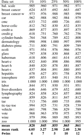
Looking at the AUC results for RBF models in Table IV
below, the overall situation is very different. For RBF models, comparing mean ranks, the best ranking ability is actually produced by using all available data when training the model. Based on statistical testing, using all data produced RBF networks with significantly higher AUC than RBF models trained using either1% or 10%.
TABLE IV
EXP. 1: LOCALLY TRAINEDRBFMODELS. AUCFOR DIFFERENT TRAINING SIZES
Data set 1% 10% 25% 50% 100% bal. scale .905 .960 .971 .982 .971 breast cancer .624 .635 .692 .663 .687 breast cancer-w .973 .976 .988 .985 .990 car .962 .988 .982 .984 .979 cmc .633 .732 .680 .726 .681 horse-colic .812 .782 .830 .832 .835 credit-a .869 .877 .855 .897 .875 credit-g .618 .751 .760 .762 .756 cylinder-bands .764 .768 .789 .822 .808 dermatology .998 .998 1.000 .997 .999 diabetes-pima .711 .800 .791 .809 .789 ecoli .971 .954 .976 .966 .976 glass .797 .838 .830 .868 .827 haberman .618 .606 .661 .614 .652 heart-c .832 .840 .898 .886 .900 heart-h .840 .820 .878 .881 .887 heart-s .837 .804 .891 .880 .895 hepatitis .678 .627 .851 .758 .878 ionosphere .895 .853 .940 .911 .954 iris 1.000 1.000 1.000 1.000 1.000 labor .844 .971 .930 .931 .951 liver-disorders .646 .646 .679 .652 .680 lymphography .824 .858 .824 .857 .868 sonar .859 .826 .811 .847 .812 tae .713 .756 .680 .735 .686 tic-tac-toe .994 .925 .731 .928 .739 vehicle .661 .798 .786 .829 .789 vote .968 .963 .970 .975 .978 wine .979 .996 .989 .985 .993 zoo 1.000 1.000 .994 1.000 .995 mean .828 .845 .855 .865 .861 mean rank 4.05 3.27 2.98 2.40 2.30 #wins 4 7 5 10 12
Summarizing the first experiment, the overall picture is that the suggested approach of training one model per instance using only local instances is almost always a better choice than building one global model using all available data. Especially when building J48 models, all smaller training sizes and local models are clearly better than the global model, both with regard to accuracy and AUC. As a matter of fact, specifically using 25% of the instances for the local training resulted in J48 models that had both significantly higher accuracy and AUC, compared to the global model. For RBF networks, the results are a bit more mixed, but using 50% to train a local model obtained clearly higher accuracy, and simlar AUC. Table V below shows the number of wins for the locally trained models, using different training sizes. The tabulated numbers are wins for locally trained models against the global model. In a pair-wise comparison over30 data sets, 20 wins are sufficient for statistical significance, using a standard sign test. Bold numbers indicate a significant number of wins for the
local technique while underlined numbers indicate a significant number of wins for the global technique.
TABLE V EXP. 1 - SUMMARY J48 RBF 1% 10% 25% 50% 1% 10% 25% 50% Accuracy 19 19 21 21 12 16 19 20 AUC 21.5 21 28.5 28.5 5 13 10 14
So, also when comparing the techniques head-to-head, all local techniques producing J48 trees obtained significantly higher AUC, compared to the global J48 model. In addition all four training sizes resulted in 19 − 21 wins with regard to accuracy; i.e., the difference in accuracy is either statis-tically significant, or quite clear. Looking at RBF models, the locally trained models using either 25% or 50% of the instances obtained19 and 20 accuracy wins against the global model, respecitively. Comparing AUCs, however, the global technique outperformed all locally trained variants. Against the techniques using either 1% or 25%, the number of wins was even enough for statistical significance.
Turning to experiment 2, Table VI below shows the accu-racy results.
TABLE VI EXP. 2 - ACCURACY
J48 RBF
Data set 100% A10 A25 CV 100% A10 A25 CV bal. scale .778 .794 .797 .862 .863 .880 .883 .885 breast cancer .743 .748 .747 .730 .714 .745 .748 .708 breast cancer-w .950 .969 .969 .967 .962 .968 .968 .968 car .922 .912 .926 .921 .888 .853 .814 .887 cmc .514 .490 .490 .511 .502 .491 .492 .531 horse-colic .852 .835 .835 .848 .803 .828 .827 .790 credit-a .856 .873 .873 .853 .796 .868 .868 .849 credit-g .712 .741 .742 .711 .737 .746 .746 .742 cylinder-bands .578 .704 .699 .717 .727 .714 .717 .761 dermatology .941 .964 .968 .978 .966 .968 .967 .965 diabetes-pima .745 .747 .745 .736 .740 .754 .750 .743 ecoli .828 .833 .843 .836 .833 .858 .851 .834 glass .676 .698 .703 .705 .649 .704 .713 .717 haberman .722 .720 .737 .719 .731 .705 .731 .714 heart-c .771 .824 .832 .793 .835 .826 .833 .827 heart-h .802 .812 .818 .791 .828 .827 .836 .819 heart-s .782 .809 .811 .775 .831 .805 .804 .828 hepatitis .792 .831 .831 .796 .853 .833 .838 .856 ionosphere .897 .860 .866 .884 .917 .857 .861 .915 iris .947 .947 .955 .943 .960 .957 .955 .949 labor .786 .899 .907 .861 .911 .927 .910 .890 liver-disorders .658 .651 .654 .641 .651 .656 .663 .646 lymphography .758 .842 .837 .810 .797 .837 .842 .817 sonar .736 .838 .845 .859 .726 .828 .832 .859 tae .574 .545 .559 .607 .498 .604 .598 .598 tic-tac-toe .853 .980 .979 .976 .709 .951 .945 .984 vehicle .723 .730 .729 .729 .654 .723 .724 .713 vote .966 .958 .959 .963 .937 .948 .950 .950 wine .932 .968 .973 .943 .977 .970 .970 .980 zoo .926 .960 .965 .939 .943 .959 .964 .956 mean .791 .816 .820 .813 .798 .820 .820 .823 mean rank 3.03 2.45 1.78 2.73 2.87 2.45 2.17 2.52 #wins 5 5 14 6 6 7 8 9
Looking at the mean ranks, the ordering is quite clear for J48 models; A25 is better than A10, which is better than using internal cross-validation. All three algorithms are, however, clearly better than the standard approach. From a Friedman test, the only statistically significant difference is that A25 obtained higher accuracy than the standard approach. For RBF models, the picture is again quite different. Here, the internal cross-validation is the most successful approach, even if the overall differences are very small.
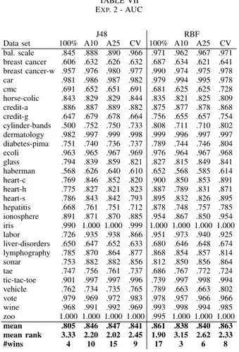
The AUC results for Experiment 2 are presented in Ta-ble VII below. Again, the results are very different for J48 and the RBF networks. When using J48 models, both A10 and A25 obtained significantly higher AUC, compared to the global model. For RBF models, however, the global model has the best ranking ability followed by using internal cross-validation, while A25 and A10 are clearly worse.
TABLE VII EXP. 2 - AUC
J48 RBF
Data set 100% A10 A25 CV 100% A10 A25 CV bal. scale .845 .888 .890 .966 .971 .962 .967 .971 breast cancer .606 .632 .626 .632 .687 .634 .621 .641 breast cancer-w .957 .976 .980 .977 .990 .974 .975 .978 car .981 .986 .987 .982 .979 .994 .995 .978 cmc .691 .652 .651 .691 .681 .625 .625 .728 horse-colic .843 .829 .829 .844 .835 .821 .825 .809 credit-a .886 .887 .889 .882 .875 .877 .878 .868 credit-g .647 .679 .678 .664 .756 .655 .657 .754 cylinder-bands .500 .752 .750 .733 .808 .711 .710 .802 dermatology .982 .997 .999 .998 .999 .996 .997 .997 diabetes-pima .751 .740 .736 .737 .789 .744 .746 .804 ecoli .963 .965 .967 .969 .976 .964 .967 .968 glass .794 .839 .859 .821 .827 .815 .849 .841 haberman .568 .626 .640 .610 .652 .568 .585 .614 heart-c .769 .846 .852 .820 .900 .850 .853 .891 heart-h .775 .827 .821 .823 .887 .789 .831 .871 heart-s .786 .843 .842 .793 .895 .832 .826 .895 hepatitis .668 .761 .751 .712 .878 .748 .757 .785 ionosphere .891 .871 .870 .885 .954 .867 .850 .954 iris .990 1.000 1.000 .999 1.000 1.000 1.000 1.000 labor .726 .935 .938 .866 .951 .973 .940 .925 liver-disorders .650 .647 .652 .633 .680 .646 .648 .674 lymphography .785 .870 .864 .877 .868 .854 .857 .814 sonar .753 .882 .882 .856 .812 .850 .856 .864 tae .747 .756 .761 .737 .686 .767 .772 .724 tic-tac-toe .901 .997 .997 .996 .739 .997 .998 .994 vehicle .762 .734 .735 .765 .789 .663 .663 .802 vote .979 .969 .972 .983 .978 .957 .966 .966 wine .968 .991 .992 .969 .993 .998 .994 .985 zoo 1.000 1.000 1.000 1.000 .995 1.000 1.000 1.000 mean .805 .846 .847 .841 .861 .838 .840 .863 mean rank 3.33 2.20 2.02 2.45 1.90 3.15 2.62 2.33 #wins 4 10 15 9 17 3 6 8
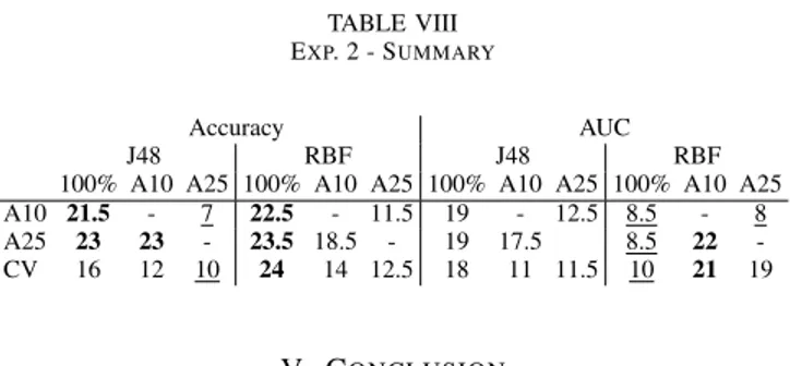
Summarizing Experiment 2 by comparing pair-wise wins in Table VIII below, the most important observation is probably that A10 and A25 obtained significantly higher accuracy than the global model, using either J48 trees or RBF networks. The internal cross-validation produced significantly more accurate RBF models, but was less successful for J48 models. Looking at AUCs, all three algorithms clearly outperformed the global model when using J48 models, but were actually significantly
worse than the global model when using RBF models.
TABLE VIII EXP. 2 - SUMMARY
Accuracy AUC
J48 RBF J48 RBF
100% A10 A25 100% A10 A25 100% A10 A25 100% A10 A25 A10 21.5 - 7 22.5 - 11.5 19 - 12.5 8.5 - 8 A25 23 23 - 23.5 18.5 - 19 17.5 8.5 22 -CV 16 12 10 24 14 12.5 18 11 11.5 10 21 19
V. CONCLUSION
In this study, different schemes for utilizing locality when inducing predictive models, in the form of standard decision trees and RBF neural networks, have been proposed and evaluated. The main idea consists of building models specific to each test instance, using only a proportion of the available training instances, selected based on locality to the test instance at hand. In Experiment 1, different proportions (ranging from 1% to 75%) of the training data were used to build the model for each test instance. The overall result from this experiment is that schemes using only a proportion of training data for model building generally yields better predictive performance than using all available training data and building a global model. There are, however, big variations between data sets and no setup consistently performs better than all the other. There is also a marked difference between the two techniques used, with the difference being more pronounced for J48 decision trees, than for RBF neural networks. Specifically, for decision trees, most local techniques producing J48 trees obtained significantly higher accuracy and AUC, compared to the global J48 model. For RBF networks, only local models using 50% of the training data obtained significantly higher accuracy than the global RBF model, and when measuring predictive performance as AUC, the global model actually outperformed all local models. This difference is especially interesting since J48 decision trees do not employ any infor-mation about locality when inducing models, whereas RBF networks utilize k-means clustering as a preprocessing step for its logistic regression. In Experiment 2, two different ways of finding a suitable proportion of instances to use for model building are evaluated. Using internal cross-validation on each fold to find a suitable proportion produced significantly more accurate RBF models, but was less successful for J48 trees. When using an iterative, but greedy, search procedure to determine the best proportion, models significantly more accurate than the global model were obtained both for J48 trees and RBF networks. The AUC results were again different for the two techniques, with J48 models found by the greedy local search being clearly better than the global model, while the global RBF model significantly outperformed all models found from the greedy search. To conclude, the experiments show that the proposed method of inducing local models improves predictive performance for both decision trees, and to a slightly lesser degree, RBF networks over a large number of data sets.
It should also be noted that the proposed method could be utilized with any type of predictive model.
VI. DISCUSSION
Building one model for each test instance is of course quite computationally expensive. At the same time, it must be noted that this process is very parallelizable. From the results it is obvious that predictive performance can be improved by using locally trained models for each instance, but it remains to investigate for which inductive techniques this applies. Finally, the fact that very different training sizes were successful for different data sets, more sophisticated schemes to find an optimal number of neighboring training instances should be developed and evaluated.
REFERENCES
[1] C. M. Bishop, Neural Networks for Pattern Recognition. Oxford University Press, November 1995.
[2] E. A. Helgee, L. Carlsson, S. Boyer, and U. Norinder, “Evaluation of quantitative structure-activity relationship modeling strategies: local and global models.” Journal of chemical information and modeling, vol. 50, no. 4, pp. 677–89, Apr. 2010.
[3] S. Zhang, A. Golbraikh, S. Oloff, H. Kohn, and A. Tropsha, “A Novel Automated Lazy Learning QSAR (ALL-QSAR) Approach: Method De-velopment, Applications, and Virtual Screening of Chemical Databases Using Validated ALL-QSAR Models,” Journal of chemical information
and modeling, vol. 46, pp. 1984–1995, 2006.
[4] X. Fern and C. Brodley, “Boosting lazy decision trees,” in Proceedings
of the Twentieth International Conference on Machine Learning, vol. 20, no. 1, 2003, pp. 178–185.
[5] D. Margineantu and T. Dietterich, “Improved class probability estimates from decision tree models,” Lecture Notes in Statistics - Nonlinear
Estiamtion and Classification, vol. 171, pp. 173–188, 2003.
[6] X. Zhu, “Bagging very weak learners with lazy local learning,” 2008
19th International Conference on Pattern Recognition, pp. 1–4, 2008. [7] Y. Yan and H. Liang, “Lazy learner on decision tree for ranking,”
International Journal on Artificial Intelligence Tools, vol. 17, no. 1, pp. 139–158, 2008.
[8] Y. C. Martin, J. L. Kofron, and L. M. Traphagen, “Do structurally similar molecules have similar biological activity?” Journal of medicinal
chemistry, vol. 45, no. 19, pp. 4350–4358, 2002.
[9] J. H. Friedman, R. Kohavi, and Y. Yun, “Lazy decision trees,” in National
Conference on Artificial Intelligence, 1996, pp. 717–724.
[10] R. Kohavi and C. Kunz, “Option decision trees with majority votes,” in
In Proc. 14th International Conference on Machine Learning, 1997, pp. 161–169.
[11] I. H. Witten and E. Frank, Data Mining: Practical Machine Learning
Tools and Techniques, Second Edition (Morgan Kaufmann Series in Data Management Systems). Morgan Kaufmann, 2005.
[12] J. R. Quinlan, C4.5: programs for machine learning. Morgan Kaufmann Publishers Inc., 1993.
[13] T. Fawcett, “An introduction to roc analysis,” Pattern Recognition
Letters, vol. 27, no. 8, pp. 861–874, 2006.
[14] A. P. Bradley, “The use of the area under the roc curve in the evaluation of machine learning algorithms,” Pattern Recognition, vol. 30, no. 7, pp. 1145–1159, 1997.
[15] A. Asuncion and D. J. Newman, “UCI machine learning repository,” 2007.
[16] J. Demšar, “Statistical comparisons of classifiers over multiple data sets,”
J. Mach. Learn. Res., vol. 7, pp. 1–30, 2006.
[17] M. Friedman, “The use of ranks to avoid the assumption of normality implicit in the analysis of variance,” Journal of American Statistical
Association, vol. 32, pp. 675–701, 1937.
[18] O. J. Dunn, “Multiple Comparisons Among Means,” Journal of the
American Statistical Association, vol. 56, no. 293, pp. 52–64, 1961. [19] P. B. Nemenyi, Distribution-free multiple comparisons. PhD-thesis.