Screening Web Breaks in a Pressroom by Soft Computing

(1)

Technical report, IDE0804, January 2008

Screening Web Breaks in a

Pressroom by Soft Computing

Master’s Thesis in Computer Systems Engineering

Ahmad Alzghoul

School of Information Science, Computer and Electrical Engineering Halmstad University

(2)

Pressroom by Soft Computing

School of Information Science, Computer and Electrical Engineering Halmstad University

Box 823, S-301 18 Halmstad, Sweden

(3)

Preface

This thesis is submitted for the degree of Master in Computer Systems En-gineering at the University of Halmstad. I would like to express my sincere thanks to my supervisor Professor A.Verikas for his guidance and help. And I am greatly indebted to my parents for their love, support and inspiration. Finally I would like to thank everyone who contributed to this project.

(4)

(5)

Abstract

Web breaks are considered as one of the most significant runnability problems in a pressroom. This work concerns the analysis of relation between various parameters (variables) characterizing the paper, printing press, the printing process and the web break occurrence. A large number of variables, 61 in total, obtained off-line as well as measured online during the printing process are used in the investigation. Each paper reel is characterized by a vector x of 61 components.

Two main approaches are explored. The first one treats the problem as a data classification task into ”break” and ”non break” classes. The procedures of classifier training, the selection of relevant input variables and the selection of hyper-parameters of the classifier are aggregated into one process based on genetic search. The second approach combines procedures of genetic search based variable selection and data mapping into a low dimensional space. The genetic search process results into a variable set providing the best mapping according to some quality function.

The empirical study was performed using data collected at a pressroom in Sweden. The total number of data points available for the experiments was equal to 309. Amongst those, only 37 data points represent the web break cases. The results of the investigations have shown that the linear relations between the independent variables and the web break frequency are not strong.

Three important groups of variables were identified, namely Lab data (variables characterizing paper properties and measured off-line in a paper mill lab), Ink registry (variables characterizing operator actions aimed to adjust ink registry) and Web tension. We found that the most important variables are: Ink registry Y LS MD (adjustments of yellow ink registry in machine direction on the lower paper side), Air permeability (character-izes paper porosity), Paper grammage, Elongation MD, and four variables characterizing web tension: Moment mean, Min sliding Mean, Web tension

variance, and Web tension mean.

(6)

the occurrence of web breaks and can also be used for solving other industrial problems.

(7)

List of Tables

2.1 The list of the Off-line data . . . 9 2.2 The list of the Online data . . . 11 5.1 The coefficient of correlation between the independent

vari-ables and the web break frequency along with the p−values lower than 0.05. . . 26 5.2 The variables included into the linear model along with values

of the model parameters, the standard errors of the parame-ters, and the z−score values. . . 26 5.3 The CCR (%) of the break and non break cases obtained for

the training and test data sets using the fitness function given by Eq. 5.1. . . 27 5.4 The CCR (%) of the break and non break cases obtained for

the training and test data sets using the fitness function given by Eq. 5.4. . . 29 5.7 The CCR (%) obtained from the k-NN classifier for the break

and non break cases along with the overall performance . . . . 30 5.8 The CCR (%) of the break and non break cases obtained for

the training and test data sets using the fitness function given by Eq. 5.5. . . 31 5.9 The CCR (%) obtained from the k-NN classifier for the break

and non break cases along with the overall performance. . . . 32 5.10 The CCR (%) of the break and non break cases obtained from

the CCA based approach for the training and test data sets using the fitness function given by Eq. 5.3. . . 33

(10)

(11)

List of Figures

1.1 The variations of load and strength plotted as probability

den-sity functions. . . 2

1.2 Web break statistics observed in heatset offset presses. . . 4

2.1 A schematic description of the sampling system. . . 12

3.1 The flowchart of the genetic search based procedure for finding the most important process variables. . . 14

4.1 The main steps of GA. . . 19

4.2 Illustration of the crossover operation. . . 20

4.3 Illustration of the mutation operation. . . 20

4.4 The optimal hyperplane (decision boundary) found by training a SVM. The hyperplane is defined by the support vectors. . . 21

5.1 Left: The first two principal components of the original data. Right: The first two principal components of the 8-dimensional data. . . 31

5.2 Left: The original data mapped onto the first two CCA com-ponents. Right: The 8-dimensional data mapped onto the first two CCA components. . . 33

(12)

(13)

Chapter 1 Introduction

1.1 Background

The steadily increasing competition forces both printers and paper makers to increase the efficiency and effectiveness of their equipment. In the print-ing industry, runnability is considered as beprint-ing one of the most important factors affecting printing process productivity. Runnability is defined as a printing process without any faults, interruptions, and stops. Web breaks, web instability, register errors and wrinkling are examples for runnability problems which affect productivity and also the quality of the products, and cause huge losses [1].

Web breaks are considered as the most significant cause of runnability problems. Web breaks occur when the total applied load on the web exceeds the strength of the web. There are two main factors affecting the occurrence of web breaks: the applied load and the web strength. Both factors vary randomly around a mean value from time to time. There are different sources causing the variation in the applied load and the web strength. Out of roundness of a paper roll, unwind rolls, and unwind stands are examples of load variation sources. While variation of grammage, formation and furnish are examples of web strength variation sources [2].

The variation of load values depends on tension set points, while the strength value variation depends on the material manufacturing process. These variations can be plotted as probability density functions, as shown in Fig. 1.1. It was shown that as the data sample size increases, the curves become more skewed and shifted towards each other. The region pounded by the overlapped curves implies the possibility of the web break occurrence. However, neither the strength nor the load can be used alone to assess the runnability. On the other hand, having low variability, high runnability can

(14)

be achieved even at low strength, while a high average strength and high variance of the strength may lead to low runnability [2].

20 40 60 80 100 0 0.01 0.02 0.03 0.04 0.05 0.06 Load Strength Probability Applied load Web strength

Figure 1.1: The variations of load and strength plotted as probability density functions.

Web breaks entail huge financial losses caused by a production stop, rang-ing between 10 and 20 minutes. This may result in the disruption of the pro-duction process due to the necessity of removing the ruined paper, rethreads, and restarting the machine. This results in financial losses in the form of costs of the corrupted web, downtime costs, and possible machinery damage [2]. Furthermore, this may result in an unsatisfied customer and, in some cases, extra penalties due to not delivering on time.

The huge losses and the need to increase the productivity without any runnabilty problems stimulate a search for the reasons behind web breaks as well as ways for solving the problem. A substantial body of research has been done in this field: see for example [1, 3], where the authors aimed to find the factors affecting runnability and attempted to control them to prevent web breaks. Actually, web breaks is a difficult problem to solve due to the rare occurrence of the breaks. It was found that the break rate can be approximated by the Poisson distribution [4]. Hence, the end points of an approximate two-sided 100(1 − α)% large sample interval for the web breaks frequency p = Nb/N are: p + z 2 1−α/2 2N ± z1−α/2_√ N q p + z2 1−α/2/(4N) (1.1)

where Nb is number of breaks, N is the total number of observations, and z1−α is the 100(1 − α) percentile of the standard normal distribution.

(15)

Introduction To highlight the problem, let us assume that N = 100 and p = 0.01. Then, from Eq. (1.1), the end points of the 95% confidence interval are 0.0018 and 0.057. This means that only web break frequencies differing more than 31.6 times can be considered as significantly different. Therefore, we need a huge number of paper rolls for a reasonable statistical analysis. An addi-tional difficulty stems from the large number of factors, which may trigger a web break such as too large variations of the paper thickness, formation, moisture, speed of the printing press, web tension, paper defects, and various parameters of the printing process. In addition, it is sometimes difficult to recognize what causes web breaks, since web breaks occasionally happen due to human faults [3].

1.2 Related work

Different methods and techniques have been used aiming to explain the rea-sons behind paper web breaks [1, 3, 5, 6]. Most of these methods focus on finding parameters which have a high correlation with web break occurrences. There are many parameters which may be responsible for runnability prob-lems. Some of these parameters are difficult to measure or even inaccessible. Therefore, some researchers use modeling and simulation to analyze the pa-per structure, the printing process, and the papa-per-press interaction, see for example, Provatas and Uesaka [3]. The authors model the paper structure and paper-press interaction analytically. The model solves the problem of inaccessible parameters, predicting values of the process parameters in each printing process step and observing the interaction between them.

Since statistical analysis gives an indication that there is a relation be-tween the machine direction (MD) tensile strength and the occurrence of the web breaks, Hristopulso and Uesaka [5] used basic physical laws to model the web dynamics. The authors concentrate their work on MD tension vari-ation in a paper web under the assumption of a constant web speed. This model aims to explore the relation between the out-of-roundness degree and web breaks, and to investigate the relation between the tension variation and web breaks. It was found that the starting-up and shutting down operations and the extreme roll deformation have a direct effect on the web tension which causes web breaks.

On the other hand, other researchers based their analysis solely on data collected during the production process. For example, Parola et al [1] gath-ered a large amount of data from a printing press and a paper mill and used data mining techniques to analyze the printing press runnability. The goal of this work was to identify the causes responsible for the runnability

(16)

prob-lems in a pressroom. Principal Component Analysis (PCA), Multiple Linear Regression, and Correlation Analysis are the methods used for data mining. Data mining increases the ability to monitor the printing process by knowing the factors affecting the process.

Miyaishi and Shimada [6] developed an artificial neural network (a multi-layer perceptron) to tackle the web breaks problem on a commercial newsprint paper machine. The network was trained to predict the occurrence of a web break. The magnitude of the network weights in the input layer has been used to reduce the number of the input variables by keeping those related to the largest input weights. Out of 41 available variables, five variables con-tributing to paper web breaks were selected. Based on the variables found, a variety of countermeasures were taken that resulted into the reduced number of web breaks and reduced fiber losses.

Printing press related factors, unknown factors, paper related factors, and other factors are the main groups of factors. Fig. 1.2 presents the distribution of paper web break factors observed in heatset offset presses [7]. As can be seen from Fig. 1.2, press related factors compose the largest group of factors trigging paper web breaks. Thus, the optimization of the press operator actions could be one of the most important measures to reduce the number of paper web breaks.

0 10 20 30 40 50 1 2 3 4 5 6

Percentage of all breaks

Reason 1 Press related 2 Unknown 3 Wrinkling 4 Mill splice 5 Winder cracks 6 Other known

Figure 1.2: Web break statistics observed in heatset offset presses. There is a huge variety of parameters which may influence the printing press and paper related factors trigging a paper web break. Previous studies have shown that the most important parameters influencing paper web break factors are: web tension, web strength, slack area in the paper, the out of

(17)

Introduction properties related to web breaks are: MD tensile strength, strain-to-failure, and the regularity of tensile strength. It is claimed that tensile strength is the most important factor affecting the web breaks and can be used to predict breaks, while the tear strength has less effect [8, 10]. However, these parameters are not so easy to control because the web tension varies from time to time, especially when a paper roll is changed. Moreover, the web strength is not constant across the whole web and sometimes the web contains holes or weaknesses and the paper properties depend on how long the paper has been stored and the environment around it. Also, different paper mills produce paper of different quality and standards.

1.3 The aim and novelty of the project

Parameters affecting the printing press related factors causing paper web breaks may be quite pressroom specific, depending on the printing press and paper interaction. However, supported by the results available from other studies, some general conclusions may also be drawn from such pressroom specific studies. Pressrooms experiencing frequent paper web breaks are valu-able information sources for such studies. This work is done using data from such a pressroom.

The project aims at finding the most important parameters causing web breaks by using soft computing techniques. Two novel approaches to pa-per web break data analysis are explored. The first one treats the problem as a task of data classification into “break ” and “non break ” classes. The procedures of classifier design and the selection of relevant input variables (features) are integrated into one process based on genetic search [11]. The search process results into a set of input variables providing the best clas-sification performance. The second approach, also based on genetic search, combines procedures of input variable selection and data mapping into a low dimensional space. The curvilinear component analysis [12] as well as the principal component analysis are employed for implementing the mapping. The genetic search process results in a variable set providing the best map-ping according to some fitness function. The fitness function used is such that the disparity between the breaks and non-breaks data is emphasized. The integration of processes of classification and variable selection or mapping and variable selection allows finding the most important variables according to the fitness functions used to assess the classification or mapping results.

(18)

(19)

Chapter 2 The pressroom and data

2.1 The press room

Today offset printing is the most common printing technology. Offset print-ing is an indirect lithographic printprint-ing technology where ink is transferred from an ink tray onto a printing plate and then onto the printing surface via a flexible blanket. Four primary colours: cyan, magenta, yellow, and black are usually used to create colour printed pictures. There is a separate printing plate four each colour. The printing and non printing areas are on the same plane of the printing plates. To distinguish between printing and non-printing areas, the printing areas are made to be ink-accepting, while the non printing areas are ink-repellent. There are two main technologies to achieve ink-repellent areas [13]:

Conventional offset printing technology When using this technology, a dampening solution is applied to the printing plate by dampen-ing rollers. The non-printdampen-ing areas are hydrophilic (water-receptive). Therefore, the ink is not transferred to these areas, since the damping solution prevents that. The printing areas are oleophilic, thus unrecep-tive to water.

Water-less offset printing technology A layer of silicon is used to make the printing plate ink-repellent. For ink-receptive areas a planed inter-ruption to the silicon area is used.

Regarding paper feed into a printing press, offset printing can be divided into two categories [13]:

Sheet-fed offset printing The printing machine is supplied with distinct pages of paper. This type of printing is used for small and medium size jobs. The printing process can run at up to 4m/s speed.

(20)

Web offset printing In web offset mode the printing press is supplied with large rolls of paper. The web width can vary to some extent. This type of printing is used for larger jobs. The printing process can run at up to 15m/s speed.

There are two types of web offset, the so called [13]:

• Coldset web, where the ink is drying due to absorption and

evap-oration. Coldset is usually used in newspaper printing.

• Heatset web, where hot air dryers are used to dry the ink.

Heat-set is often used in commercial printing, since the paper used in commercial printing is often less absorbent.

In this project, a four colour (cyan, magenta, yellow, and black) heatset web offset printing press has been used to collect the data. The press can run at up to 10m/s speed. The paper roll width can vary between 44 and 96

cm.

2.2 The data

There are two types of data, data obtained before running the printing press,

Off-line data, and data collected during the printing process, On-line data.

The off-line variables are categorized into several groups. Lab data, moisture content, defects, roll machine data, time from service, speed, tambor position, washing, and others are the groups of off-line variables. Table 2.1 presents the complete list of the off-line variables: MD stands for machine direction and CD stands for cross-direction. Below we give a short description of the variables, as their names are not self-explanatory.

Lab data are obtained at a paper mil lab and reflect various paper prop-erties. DIP content means the percentage of recycled fibers in the pulp, SBK content evaluates the percentage of the sulphate type pulp. Formation index assesses the tendency of fibers to make clusters. Paper roughness is estimated for the lower side (LS) and upper side (US) using two different air pressure rates. The defects registered in the paper are black scribbles, holes, attenua-tion, dark and light spots and others. The direction variable in the Tambor position group takes the value of 1 if it is the edge roll and 0 otherwise. The variables from the roll machine group characterize the winding hardness and speed.

Web break frequency, web width, ink registry, main registry, web tension, and moisture content are the categories of the on-line variables. Table 2.2 presents the complete list of the on-line variables. Mostly, the maximum

(21)

The pressroom and data Table 2.1: The list of the Off-line data

Group Feature name Unit Index Lab data Tensile Index, MD Nm/g 85

Tensile Index, CD Nm/g 86 DIP Content % 87 SBK Content % 88 Starch Content Kg/ton 89 Formation – 90 Ash Content % 91 Tear strength, CD mN 92 Roughness 1kg LS ml/min 93 Roughness 1kg US ml/min 94 Roughness 5kg LS ml/min 95 Roughness 5kg US ml/min 96 Air permeability Ml/min 97 Anisotropy – 98 Elongation, MD % 99 Pinhole Area PPM 100 Moisture content 101 Grammage g/m2 ₁₀₂

Printing speed # Changes Count 108 Dominating speed Revs/hour 109 Defects # Of defects found Count 110 Roll machine Hardness, mean 115 Hardness, variance 116 Speed, mean 117 Speed, variance 118 Others Time from service Hours 120 Runtime from service Hours 121 Roll age Days 122 Tambor position Direction 0/1 123 Distance from centre, CD m 124 frequency of the web break is two, since the roll will be changed after that. In the Ink registry group of variables, Y refers to the registry values for the yellow colour, and US and LS refer to the upper and lower paper side, respectively. The parameter k describes the slope of the line fitted to the ink registry adjustment data, separately for the MD and CD adjustments. The same explanation applies to the Main registry group of variables. The number

(22)

of adjustments is counted during the entire printing duration for a given paper roll. The variables in the Web tension axis 1 group are obtained from the web tension measurements made before the printing nip. The other group of web tension variables are obtained from the web tension measurements made after the printing nip. The last two variables in the Web tension axis 2 group are calculated in a sliding window.

The Moisture content group of variables characterize the adjustments made of the left- and the right-hand of the paper web to compensate for moisture deviation from the predetermined level. The adjustments are made in discrete moisture units.

Fig. 2.1 presents a schematic description of the sampling system used to collect the online data. The UNISET 2 illustrates the printing press used. The bar code reader connected to the sampling system through RS485 via TCP/IP reads the paper reel ID code. The ID code allows linking the online data with the off-line data obtained from a paper mill. The linked data are stored in a database. The press control system is connected to both the control unit and the sampling system via ARCNET. The registry data are obtained via this connection. Finally, the Damp unit is connected to both the Spray bars through RS485 and the control unit through RS422. The moisture content data are obtained via this connection. Although not shown in the scheme, the web break frequency and the web tension data are also logged in the database.

There are 61 independent variables in total and the total number of data points available for the experiments were 309. Amongst those, only 37 data points represent the web break cases. Thus, there are very few data points representing the break class. Moreover, not all the 61 variables were available for all the 307 paper reels investigated. All the 61 variables were available only for 87 reels containing 11 break cases. Therefore single groups and several groups of variables have been used in different experiments. For example, by removing the web width group of variables, we increased the size of the data matrix X from 87 × 61 to 148 × 57. Therefore, this data matrix was the main data set used in the experiments. There were 18 break cases in this set of data. Thus, the data set used contains all the groups of variables presented in Table 2.1 and Table 2.2, except the Web width group of variables. Note that if we end with variables which belong to less number of groups, then we do the experiment again using only these variables. Due to that the number of data points may be increased, for example by using the variables from the Lab data, Ink registry, and Web tension groups, the number of data points increased to 213 with 28 break cases.

(23)

The pressroom and data

Table 2.2: The list of the Online data

Group Feature name Unit Index Web break frequency Frequency Count 1 Web width Width, mean mm 2 Width, variance mm 3 Position, mean mm 4 Position, variance mm 5 Ink registry Y, US MD, (k) 6 MD, # adjustments Count 7 CD, (k) 8 CD, # adjustments Count 9 Ink registry Y, LS MD, (k) 10 MD, # adjustments Count 11 CD, (k) 12 CD, # adjustments Count 13 Main registry MD, (k) 14 MD, # adjustments Count 15 CD, (k) 16 CD, # adjustments Count 17 Web tension, axis 1 Web tension, mean N 18 Web tension, variance N 19 Moment, mean N 20 Moment, variance N 21 Web tension, axis 2 Web tension, mean N 22 Web tension, variance N 23 Moment, mean N 24 Moment, variance N 25 Min sliding Mean N 26 Max sliding Mean N 27 Moisture content Sum left, mean 103

Sum right, mean 104 Sum all, mean 105 Difference l-r, mean 106 # adjustments Count 107

(24)

(25)

Chapter 3 The approach

We start our work by exploring linear relations between the independent and the dependent variables. All the variables discussed in the previous chapter are independent, except one—web break occurrence—which is the dependent variable. The existence of strong linear relations indicates a possibility of finding an appropriate solution based on a simple linear model.

Next, two genetic search based approaches are applied. In the first one, the task is considered as a two-class (break, non-break ) classification problem. In the second approach, relations between various process parameters and the web break occurrence are explored through mapping the multi-variable process data into a low dimensional space.

3.1 Exploring linear relations

Correlation analysis and the multivariate linear regression are the two tech-niques used to examine the linear relations. We use the Person’s correlation coefficient to assess the strength and direction of the linear relationships. To estimate the parameters of the linear model, the least squares technique is applied.

3.2 Genetic search based approach

As it has already been discussed, the project aims at finding the most im-portant variables affecting the occurrence of web breaks. Genetic algorithms (GA) are known as being capable of finding an optimal solution in various optimization problems. Therefore, we utilize GA in both the classification and mapping based techniques in order to explore relations between var-ious process parameters and web breaks occurrence. Given a long enough

(26)

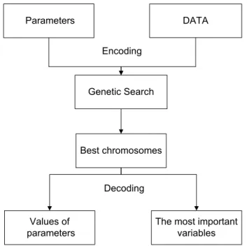
search time, not only the optimal variable subset, but also the optimal hyper-parameters of the techniques can be found during the genetic search. Fig. 3.1 presents the flowchart of the genetic search based procedure used to find the most important process variables.

Best chromosomes

The most important variables Decoding Encoding DATA Parameters Values of parameters Genetic Search

Figure 3.1: The flowchart of the genetic search based procedure for finding the most important process variables.

Process variables as well as hyper-parameters governing the behaviour of the classifier or the mapping technique are encoded into the so-called chromosomes and are presented together with the process data to the genetic search procedure. The genetic search results into a set of best chromosomes containing information on the most important variables and the values of the hyper-parameters. As mentioned above, the genetic search is based either on classification or mapping into a low-dimensional space and aims at finding the optimal set of variables according to some quality (fitness) function. A more thorough description of the genetic search process will be given in the next chapter.

3.2.1 Classification based genetic search

In this case, the problem is treated as a task of data classification into break and non break classes. During the genetic search a classifier is designed using

(27)

The approach

N labelled samples. Since both hyper-parameters of a classifier and input

variables are encoded in a chromosome, the procedures of classifier design and the selection of relevant input variables (features) are integrated into one process, based on genetic search. Since the correct classification rate of the test set data constitutes the fitness function used during the search, the search process results into a set of input variables providing the best classification performance.

In general, classifiers can be categorized into three main groups: based on similarity, probabilistic approach, and classifiers constructing decision bound-aries. The first approach is straightforward. An example of this approach is template matching. The second approach relies on Bayes decision rule [14]. The k-nearest neighbor (k-NN) and the Parzen window classifier are exam-ples for this approach [14]. The third approach makes decision boundaries depend on the minimization of some error criterion. A multilayer perceptron (MLP) and a support vector machine (SVM) are two popular examples for this approach [15]. A classifier of this type is well-suited for integration into the genetic search process.

SVM is one of the most successful and popular classifiers. SVM separates two different classes by constructing a hyper-plane maximizing the margin, i.e. the distance between the closest data points of opposite classes. The advantages of SVM are the following: the ability to find the global maxi-mum of the objective function, no assumptions made about the data, the complexity of SVM depends on the number of support vectors, but not on the dimensionality of the transformed space [14, 16, 15]. Therefore, we have chosen SVM as a base classifier in this work. A short description of the SVM classifier is given in the next chapter. Several other authors have also used GA for SVM design [17] and SVM designed integrated with variable selection [18].

3.2.2 Mapping based genetic search

In this approach, relations between various process variables and the web break occurrence are explored through mapping the multi-variable process data into a two-dimensional space. We expect that the web break and non break cases will be mapped into more or less distinctive areas of the space. The process of the emergence of separate clusters of break and non break cases is promoted in the genetic search based mapping process through the optimization of a specifically designed fitness function. Again the processes of discovering the mapping and variable selection are combined based on a genetic search. The search aims at finding the optimal feature subset according to the fitness function. The fitness function applied to assess the

(28)

mapping quality is the correct classification rate (CCR) of the test set data represented by the two space components. Two classifiers, SVM and kNN, are used to make the classification.

Mapping techniques can be categorized as being linear or nonlinear. Lin-ear methods suppose that the data set takes the shape of a linLin-ear manifold, while nonlinear methods assume that the manifold is nonlinear. There are many methods of both types. Principal Component Analysis (PCA) and Lin-ear Discriminant Analysis (LDA) are examples of linLin-ear techniques. Multi-Dimensional Scaling (MDS), Self-Organizing Map (SOM) [19], Curvilinear Component Analysis (CCA), Locally Linear Coordination (LLC), Locally Linear Embedding (LLE), and Stochastic Neighborhood Embedding (SNE) are the most prominent examples of nonlinear techniques [20].

PCA is the most popular linear mapping technique and often outperforms other linear methods. For example, Martinez [21] demonstrated that PCA outperforms LDA when training data sets are small. We have also used this linear mapping technique.

Previous studies have shown that CCA outperforms other nonlinear tech-niques, such as MDS, performing similar tasks. CCA functions as a ”self-organized neural network performing two tasks: vector quantization of the sub-manifold in the data set (input space) and nonlinear projection of these quantizing vectors towards an output space” [12]. If we compare CCA and SOM, which is a famous mapping technique, we find that SOM does not preserve the original form of the sub-manifold, while CCA preserves both the local topology and the global shape of the sub-manifold. Comparing CCA with Sheppard’s nonlinear MDS, we will find that MDS requires a lot of computation time because of its complex cost function. In addition, the cost function is highly sensitive to noise and can not escape from local min-ima [12]. Since previous studies have shown that CCA has many advantages over other nonlinear methods performing similar tasks, we have chosen CCA as a nonlinear mapping technique.

Other researchers have also attempted to combine mapping techniques with GA in order to improve the overall performance of mapping techniques. For example, Polani and Uthmann [22] used GA to find the appropriate topology of SOM, while Tanaka et al. [23] applied GA to optimize the SOM weights.

(29)

Chapter 4 Methods and techniques

4.1 Exploring linear relations

4.1.1 Correlation

Correlation analysis is a statistical technique used to measure the strength and the tendency of a linear relationship between two variables x and y. The correlation coefficient r ranges between −1 and +1 [24]

r = P_N i=1(xi− ¯x)(yi− ¯y) qP_N i=1(xi− ¯x)2 qP_N i=1(yi− ¯y)2 i = 1, 2, ..., N (4.1)

where N is the number of data points and ¯x, ¯y are the mean of x and y

respectively.

As the variables are more related, the absolute value of r increases. A positive r value indicates a directly proportionality of the variables, while a negative value indicates an inverse proportionality.

In this project, in order to determine the statistical significance of com-puted correlation coefficient values, the p − values have been used. The

p − value expresses the probability of obtaining the computed value of the

correlation coefficient by chance.

4.1.2 Linear regression model

We use the linear regression model to predict the output y, usually called de-pendent variable, using a vector x = (x1, x2, ..., xn) of independent variables.

(30)

The linear regression model can be written as [25]: y = β0+ n X j=1 xnβn (4.2)

where βi are parameters of the model. The optimal values of the parameters

found by the least square technique are given by [25]:

β = (XTX)−1XTy (4.3)

where X is a N × n matrix of input data and y is the N-vector output. To test the statistical significance of a particular parameter βj, we use

the standardized coefficient (z − score) [25]

zj = βj σpdj

(4.4) where dj is the j diagonal element of the matrix (XTX)−1 and σ is the

standard deviation of the noise. If we assume that σ is known, then zj has a

standard normal distribution and a 1 − 2α confidence interval for βj is

(βj − z(1−α)σ

p

dj, βj+ z(1−α)σ

p

dj) (4.5)

where z(1−α) _{is the 1 − α percentile of the normal distribution, for example} z(1−0.025) _{= 1.96. Thus, the approximate 95% confidence interval is given by} βj± 2σ

p

dj.

4.2 Genetic search

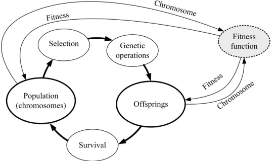
The idea of GA was first suggested by Holland and his associates in the 1960s [11]. GA is a search technique for solving optimization problems. En-coding, initialization, evaluation, selection and genetic operations represent the main steps of GA. The most important issues to consider when solving a problem by GA are encoding and evaluation, where the genetic represen-tation of the problem and the fitness function for evaluating the suggested solution are defined [26, 27]. Fig. 4.1 illustrates the main steps of GA.

Once the encoding and evaluation parts are defined, GA starts a random generating process of the population of the probable solutions in the form of chromosomes. Each chromosome consists of a string of random numbers, usually binary numbers, representing genes.

In this work, the chromosome is divided into three parts. One part is related to data (encodes the presents/absence of the input variables) and the

(31)

Methods and techniques

Figure 4.1: The main steps of GA.

other two parts are related to hyper-parameters (in the case of SVM, one encodes the value of the regularization constant C and the other encodes a kernel parameter, for example the kernel width σ when using Gaussian ker-nels). A binary encoding scheme has been used in this work. To generate the initial population, the values of the SVM parameters are selected ran-domly from predefined intervals, while a random mask string is created in order to select the input variables.

A predefined fitness function is used to make an evaluation for the generated chromosomes. We used the CCR of the test set data as a fit-ness function. Observe that in the mapping based genetic search, the CCR is evaluated using the mapped two-dimensional data. Based on the fitness values, the chromosomes are selected, usually the selection of a chromo-some probability is proportional to its fitness value. The genetic operations crossover and mutation are applied to the selected chromosomes, resulting in a new generation or population.

In crossover, pairs of parents are combined to create new chromosomes called offspring, as shown in Fig. 4.2. By applying crossover to the generated offsprings iteratively, it is expected that a generation of good chromosomes leading to good better solution will be created.

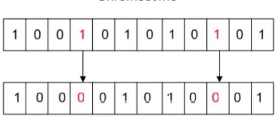
In mutation, random changes on the genes are introduced. The rate of mutation changes is proportional to the length of the chromosome. Fig. 4.3 illustrates the mutation operation on a chromosome, where the genes shown

(32)

Figure 4.2: Illustration of the crossover operation.

in red have been changed. By doing crossover iteratively a good solution can be found, while a mutation operation can be used to escape from local optima [28]. The genetic operations are applied to chromosomes with the probability of crossover pc and mutation pm. Chromosomes are included into

a new population with the probability of reproduction pr. These probabilities

governed the genetic search process.

Figure 4.3: Illustration of the mutation operation.

4.3 Support vector machine

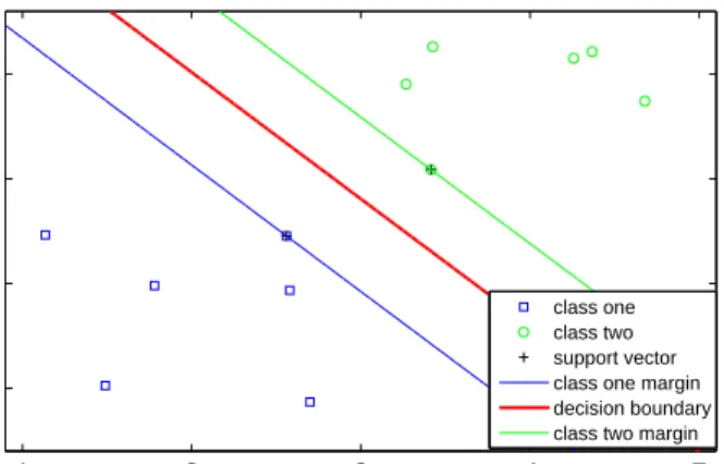
Typically, a support vector machine relies on representing the data in a new high dimension space more than in the original. By mapping the data into the new space SVM aims at finding a hyper-plane, which classifies the data into two categories. The support vectors are the closest to the hyperplane patterns from the two classes in the transformed training data set. The support vectors are responsible for defining the hyper-plane [14]. Fig. 4.4 illustrates the hyperplane (decision boundary) found by training a SVM,

(33)

Methods and techniques where the crosses (+) indicate the support vectors. One needs to find the nonlinear mapping function appropriate for the problem at hand. Polynomial and Gaussian are examples of nonlinear kernel functions used to implement the non-linear data mapping.

1 2 3 4 5 1 2 3 4 X1 X2 class one class two support vector class one margin decision boundary class two margin

Figure 4.4: The optimal hyperplane (decision boundary) found by training a SVM. The hyperplane is defined by the support vectors.

Depending on the definition of the optimization problem, several forms of SVM can be distinguished, for example, 1-norm or 2-norm SVM. Since there are examples demonstrating that the 1-norm SVM outperforms the 2-norm, especially if there are redundant noise features [29], the 1-norm SVM is used in this work. Assuming that Φ(x) is the non-linear mapping of the data point x into the new space, the 1-norm soft margin SVM can be constructed by solving the following minimization problem [30]:

min w,b,γ,ξ−γ + C N X i=1 ξi (4.6) Subject to yi(hw, Φ(xi)i + b) ≥ γ − ξi, ξi ≥ 0, k w k2= 1, i = 1, ..., N (4.7)

where w is the weight vector, yi = ±1 is the desired output (non break −1

and break +1), N is the number of training data points, hi stands for the inner product, γ is the margin, ξi are the slack variables, b is the threshold,

and C is the regularization constant controlling the trade-off between the margin and the slack variables.

(34)

The discriminant function for a new data point x is given by [30]: f (x) = H[ N X i=1 α∗ iyjk(x, xi)+b], (4.8)

where k(x, xi) stands for the kernel, and the Heaviside function H[y(x)] = −1, if y(x) ≤ 0 and H[y(x)] = 1 otherwise. In this work, the Gaussian

kernels have been used. The optimal values of the parameters α∗

i and b are

found by maximizing the following function [30].

W (α) = − N X i,j=1 αiαjyiyjk(xi, xj) (4.9) subject to N X i=1 αiyi = 0, N X i=1 αi = 1, 0 ≤ αi ≤ C, i = 1, ..., N (4.10)

4.4 k-nearest neighbor classifier

The k-NN classifier is considered as one of the simplest classification tech-niques. The popularity of this method comes from the fact that the error of the k-NN is bounded by twice the Bayes error [14]. Therefore, if there is a sample of an infinite size, the k-NN error will be less than twice the Bayes error rate. The k-NN classifies data points based on the plurality of its k closest neighbours of the training set. To measure the distance between the test data point and the training samples the Euclidian distance is generally used. Usually the value of k is chosen to be odd, to prevent the occurrence of tie salutations, especially if the problem has two classes [31].

In this project, the k-NN classifier has been used in the mapping-based genetic search, to assess the correct classification rate of the mapped two-dimensional data. The suitable value of k has been found experimentally and the Euclidian distance measure has been used to measure the distance between two data points.

4.5 Principal component analysis

PCA is an unsupervised linear dimensionality reduction technique. PCA projects the data onto the orthogonal directions of maximal variance. The

(35)

Methods and techniques projection accounting for most of the data variance is called the first principal component [32, 33].

Let X be the data matrix of size N × n, where N is the number of data points and n stands for data dimensionality. Then by applying PCA one can obtain an optimal linear mapping, in the least square sense, of the n-dimensional data on q ≤ n dimensions. The mapping result is the data matrix Z [32]:

Z = XVq (4.11)

where Vq is the n × q matrix of the first q eigenvectors of the correlation

matrix SX = _{N −1}1 XTX corresponding to the q largest eigenvalues λi, i =

1, ..., q. Then, the correlation matrix of the transformed data [32]: SZ = 1 N − 1Z T_{Z = diag{λ} 1, . . . , λq} (4.12) is a diagonal matrix.

The diagonal elements λi can be used to calculate the minimum

mean-square error (MMSE) owing to mapping the data into the q-dimensional space [32]: MMSE = n X i=q+1 λi (4.13)

4.6 Curvilinear Component Analysis

Curvilinear Component Analysis is a nonlinear dimensionality reduction strat-egy, in which the data are mapped from a high n-dimensional space to a low dimensional space with q dimensions, where q ≤ n. CCA aims to map the data in such a way that local topology is preserved. The mapping is im-plemented by minimizing a cost function based on matching the inter-point distances in the input and output spaces [12, 34].

Let the Euclidean distances between a pair of data points (i, j) be denoted as χij = d(xi, xj) and ζij = d(yi, yj) in the input and the output space,

respectively. Then, the cost function minimized to obtain the mapping is given by [12]: E = 1 2 X i X j6=i (χij − ζij)2F (ζij, λy) = 1 2 X i X j6=i Eij (4.14)

(36)

where the weighting function F (ζij, λy) is used to favor local topology

preser-vation. F (ζij, λy) should be a bounded and decreasing function. For example,

a sigmoid, unit step function, decreasing exponential or Lorentz function [12]. To minimize the cost function, Eq.(4.14), a new method is used. Given a randomly chosen data point i, the adaptation rule for the jth data point yj

in the output space is as follows [12]:

∆yj(i) = α(t)∇iEij = −α(t)∇jEij (4.15)

where α(t) decreases with time, for example α(t) = α0/(1 + t) [12].

Consid-ering a quantized weighting function (∂F /∂ζij = 0) a simple adaptation rule

is obtained [12]:

∆yj = α(t)F (ζij, λy)(χij − ζij)

yj − yi ζij

∀j 6= i (4.16)

It was found that the new procedure of minimizing the cost function saves a terrific amount of calculation time. Secondly, the procedure could escape from the local minima, and finally the final cost was lower than the cost achieved using ordinary gradient based techniques [12].

(37)

Chapter 5 Experimental investigations

In all the tests, we repeat the experiments 10 times using different random partitions of the data set into training 70% and test 30% sets. The results presented are the average values calculated from these 10 runs. In the genetic search based approaches, the predefined search intervals have been used to limit the search space of the appropriate parameter values, for example the kernel width σ and the regularization constant C. The Gaussian kernels have been used in this work. The following values of crossover, mutation and reproduction probabilities have been used: pc= 0.1, pm= 0.1, and pr = 0.01

in the genetic search process.

We start our experimental tests by exploring linear relations between the independent and dependent variables. After that, two genetic search based approaches are investigated.

5.1 Exploring linear relations

We measure the linear correlation between the independent variables and the web break frequency. Table 5.1 presents the correlation coefficients and the p−values for the variables exhibiting the p−values lower than 0.05. The

p−value expresses the probability of obtaining such a correlation by chance.

As can be seen from Table 5.1, the variables come from the three main groups of variables: printing speed, ink registry, and web tension. Moreover, most of the variables (about 73%) belong to the web tension group, indicating the importance of this type of online variables. However, the correlation coefficient values for all the variables presented in the table are relatively low, meaning that the linear relations between the independent variables and the web break frequency are not strong.

(38)

inde-Table 5.1: The coefficient of correlation between the independent variables and the web break frequency along with the p−values lower than 0.05.

Variable r p-value 108 0.31 10×10−5 6 -0.27 7.5×10−4 10 -0.30 2.5×10−4 18 -0.35 1.2×10−5 19 0.40 6.7×10−7 21 -0.21 0.0109 22 -0.18 0.0266 23 0.35 1.2×10−5 25 0.24 0.0029 26 -0.28 6×10−4 27 0.24 0.0028

pendent variables. The significance of the variables to be included into the model has been tested by calculating the z−score (Eq.4.4) for the estimated components of the parameter vector β. To select the appropriate model size, we used the stepwise elimination of model parameters. Only the variables significant at the 95% confidence level (z−score> 1.96) were included into the model. By applying this approach we ended up with 5 variables: 10, 18, 19, 21 and 124. Table 5.2 presents the selected variables, the estimated val-ues of the components of the parameter vector β of the model, the standard errors of the components, and the z−score values.

Table 5.2: The variables included into the linear model along with values of the model parameters, the standard errors of the parameters, and the

z−score values.

Variable β Standard error of β z−score

124 -0.0495 0.0235 -2.1068 10 -0.0896 0.0237 -3.7839 18 0.1797 0.0779 2.3055 19 0.2830 0.0758 3.7351 21 -0.0517 0.0253 -2.0447 As can be seen from Table 5.2, the final model contains 5 variables repre-senting the tambor position (124), ink registry (10), and the web tension axis

(39)

Experimental investigations were found by the correlation analysis. The root mean squared error (RMSE) for this model is 0.2824. This RMSE can be compared with RMSE = 0.3280 obtained for the model containing all the available variables. The mean of the absolute value of the prediction error of the model is 0.1779, while this error for the predictions always using the mean value of the dependent vari-able (the basic error rate) is 0.2137. Thus, the linear model reduces the basic error rate by only 16.73%. Based on these tests we conclude that the linear model is not appropriate for solving the problem.

5.2 Classification based genetic search

In the classification based genetic search approach, the problem is treated as a task of data classification into break and non break classes. The SVM has been used as a classifier. We started the experiments by using the following fitness function (FF):

FF = #CCBC + #CCNBC

#Test data (5.1) where #CCBC and #CCNBC is the number of correctly classified break and non-break cases, respectively, from the test data set, and #Test data is the number of data points in the test data set.

On average, the search ended with 5 variables: 10, 26, 97, 101 and 102. These variables represent the Lab (97, 101, 102), Ink registry (10) and Web

tension axis 2 (26) groups of variables. The average CCR of 90.77% was

obtained using 54 support vectors. Table 5.3 provides the CCR for both break and non-break cases coming from the training and test data sets. Table 5.3: The CCR (%) of the break and non break cases obtained for the training and test data sets using the fitness function given by Eq. 5.1.

Case Train Test Break 80.53 46.67 Non break 99.46 97.85 Total 97.03 90.77

As can be seen from Table 5.3, the CCR obtained for the break cases is much lower than the CCR obtained for the non-break ones. This can be explained by the much lower number of break cases available. There were 56 non-break and 9 break cases in the test data set. Approximately the same

(40)

proportion of the break and non-break cases (1:6) has also been observed in training data sets. Therefore, in the experiment, the importance of the break cases was increased. The following fitness function has been applied:

FF = 6 × #CCBC + #CCNBC (5.2) Four variables: 10, 26, 97 and 99 were found using this fitness function. As before, these variables represent the Lab, Ink registry and Web tension groups of variables. Table 5.4 summarizes the CCR obtained using the selected variables.

Table 5.4: The CCR (%) of the break and non break cases obtained for the training and test data sets using the fitness function given by Eq. 5.2.

Case Train Test Break 81.05 51.11 Non break 100 96.43 Total 97.57 90.15

As can be seen from Table 5.3 and Table 5.4, the CCR for the break cases increased by 4.44%, while the CCR for the non break cases decreased by 1.5%. Since we aim at increasing the percentage of correctly classified break cases, we based the FF solely on CCBC in the next experiment:

FF = #CCBC (5.3)

When using this fitness function, four variables: 10, 20, 22 and 97 have been found during the genetic search. Again, these variables represent the Lab,

Ink registry, and Web tension groups of variables. Table 5.5 summarizes the

CCR obtained from the SVM trained using this set of variables.

As can be seen from Table 5.5, the increase of the correct classification rate of the break cases if compared to case of using the fitness function given by Eq. 5.2, the overall CCR decreased significantly. Approximately the same

(41)

Experimental investigations number of support vectors have been used in the experiments using the three aforementioned fitness functions.

A large number of support vectors found usually leads to complicated, highly non-linear decision boundaries. By contrast, we aim at finding a set of variables leading to simple and compact regions of the variable space separately enclosing break and non-break cases. To find such simple compact regions of the variable space, we constrain the number of support vectors used to define the decision boundaries. We implement the constraint by adding the additional term to the fitness function given by Eq. 5.3

FF = #CCBC + ν

#SV (5.4)

where #SV is the number of support vectors and the value of the parameter

ν is found experimentally (ν = 3).

When using this fitness function, we started the search process from the best model found so far (variables 10, 26, 97, and 99). The search process ended with the same variables and a slightly lower number of support vec-tors used to define the decision boundaries. The average number of support vectors was equal to 49.5. The values of the hyper-parameters characterizing the SVM classifier were also different. Table 5.6 presents the average CCR obtained from the classifier. As can be seen, there is a big difference between the correct classification rate obtained for the training and test break cases. This fact has been observed in all the tests and can be explained by a very small number of break cases available.

Summarizing the results of the tests we can state that the most often se-lected variables are: Air permeability (97), Elongation MD (99), Ink registry

Y, LS (10), and Min sliding mean (26). These variables represent the Lab, Ink registry, and Web tension groups of variables. The variables 97 and 10

(42)

5.3 Mapping based genetic search

Two mapping approaches were explored, a linear PCA based mapping and a non-linear one based on CCA.

5.3.1 PCA based genetic search

In the first test, a k−NN has been used as a classifier for categorizing the break and non-break cases represented by the first two principal components. The value of k was found experimentally by testing k = 1, 3, 5, and 7. The fitness function given by Eq. 5.3 has been used in this experiment. Table 5.7 presents the results obtained for the different k values.

Table 5.7: The CCR (%) obtained from the k-NN classifier for the break and non break cases along with the overall performance

Model Break case Non break case Overall performance 1-NN 33.33 83.93 76.92

3-NN 33.33 89.29 81.54 5-NN 66.67 98.21 93.85 7-NN 22.22 92.86 83.08

As can be seen, the model with k = 5 achieves the highest performance. By using this model k = 5, 6 out of 9 break cases, and 55 out of 56 non break cases were classified correctly. Eight variables have been selected when using this model: 6, 13, 16, 19, 20, 25, 99 and 101. As before, these variables rep-resent the Lab, Ink registry, and Web tension groups of variables. However, only two variables, 20 and 99 have also been selected by the classification based genetic search approach.

In the second test, the SVM has been used to classify the mapped data along with the following fitness function utilized in the genetic search

FF = 6 × #CCBC + #CCNBC + ν

#SV (5.5)

where the value of the parameter ν was found experimentally and was equal to ν = 8. The search process ended with 8 variables: 90, 102, 8, 10, 12, 16, 23 and 27, representing the Lab, Ink registry, and Web tension groups of variables. Table 5.8 presents the CCR obtained from the model. As it can be seen, the CCR of the break cases obtained in the transformed space is significantly lower than that achieved in the classification based approach, see for example Table 5.6. Therefore, one can expect that there are no clear

(43)

Experimental investigations distinct regions of break and non break cases in the transformed space. The plots of the data onto the space spanned by the first two eigenvectors of the data covariance matrix substantiate this fact.

Fig. 5.1 presents two plots of the data onto the first two eigenvectors of the data covariance matrix. The left-hand side plot was obtained using all the original variables to calculate PC(s), while Fig. 5.1 (right) presents the mapping, where only the selected variables 8, 10, 12, 16, 23, 27, 90 and 102, were used to calculate the principal components. In the right-hand side plot in red the decision boundaries of the classes are shown along with the class margins. −2 0 2 −5 0 5 10 1st Principal Component 2nd Principal Component Break class Non Break class

−2 0 2 −3 −2 −1 0 1 2 3 1st Principal Component 2nd Principal Component

Figure 5.1: Left: The first two principal components of the original data. Right: The first two principal components of the 8-dimensional data.

As we can see from Fig. 5.1, there are no clear regions of break and non break cases. While some clustering tendency appears when using data of the reduced dimensionality, the degree of overlap is still high, as it is obvious from the obtained 48.89% classification accuracy of the break cases.

The application of the two classifiers, k−NN and SVM, in the PCA based genetic search approach resulted into two different variable subsets with only

(44)

one common variable (16). This fact indicates that for a given data set, there are no variables with strong relations with the web break frequency. There is weak contribution from several variables. On the other hand, in most of the cases, the selected variables come from the three groups of variables mentioned above, namely, Lab data, Ink registry, and Web tension. Compar-ing the variables selected in the classification based and PCA based genetic search approaches we find 5 common variables, namely 10, 20, 99, 101 and 102.

5.3.2 CCA based genetic search

As in the PCA based genetic search approach, two classifiers, k−NN and SVM, have been used. The fitness function given by Eq. 5.3 has been uti-lized in the search process when using the k−NN classifier to categorize the mapped data. Since, depending on initial conditions, CCA produces different results for different runs, the results were averaged over 5 runs. As before, the value of k was found experimentally. Table 5.7 presents the results obtained for the different k values.

Table 5.9: The CCR (%) obtained from the k-NN classifier for the break and non break cases along with the overall performance.

Model Break case Non break case Overall performance 1-NN 48.89 76.79 72.92

3-NN 67.78 71.43 70.92 5-NN 83.33 75.89 76.92 7-NN 72.22 92.86 90.00

As can be seen from Table 5.9, the 7-NN classifier achieved the highest overall performance. This model also selected five variables: 10, 26, 88, 100 and 102, on average, correctly classified 6.5 out of 9 break cases and 52 out of 56 non break cases. On the other hand, the highest CCR (83%) for the break cases was achieved by the 5-NN classifier. This model selected five variables: 10, 20, 93, 97 and 99. Thus, there is only one common variable (10) selected using the 5-NN and 7-NN classifiers.

In the next test, a SVM was used as a classifier. Several fitness functions presented in the previous sections were explored. The fitness function given by Eq. 5.3 provided the highest CCR. Eight variables: 9, 10, 20, 22, 86, 88, 97 and 102 were selected. Table. 5.10 summarizes the results obtained from this model.

(45)

Experimental investigations Table 5.10: The CCR (%) of the break and non break cases obtained from the CCA based approach for the training and test data sets using the fitness function given by Eq. 5.3.

On average, the model classifies correctly 5.3 out of 9 break cases and 53.1 out of 56 non break cases and uses 44.4 support vectors. The CCR obtained for the test break cases is higher than that achieved for the break cases in any other experiment involving a SVM. Fig. 5.2 presents the nonlinear mapping of the data obtained by the CCA technique. In the left-hand side plot all the original variables are used to create the 2D mapping, while only the selected variables 9, 10, 20, 22, 86, 88, 97 and 102 are used to create the right-hand side plot. The lines shown in the right-hand side plot illustrate the decision boundary and the class margins found by the SVM.

−20 −10 0 10 20 −20 −10 0 10 20 1st CCA Component 2nd CCA Component Break class Non Break class

−5 0 5 −2 0 2 4 6 1st CCA Component 2nd CCA Component

Figure 5.2: Left: The original data mapped onto the first two CCA com-ponents. Right: The 8-dimensional data mapped onto the first two CCA components.

As we can see from Fig. 5.2, the mapping created using only the selected variables exhibits a clearer clustering tendency of the break and non break cases than that exploiting all the original variables. However, the clustering tendency revealed in the 2D space is not strong enough for drawing clear conclusions. Comparing the results obtained from the k-NN and SVM clas-sifiers, we find that there are 5 common variables: 10, 20, 88, 97 and 102.

(46)

However, when considering all the three classifiers, 5-NN, 7-NN and SVM separately, only one common variable (10) is obtained. Table 5.11 presents the variables selected by the different techniques.

Table 5.11: The variables selected by the different techniques. Method Variables

Linear relations Correlation anal. 6 10 18 19 21 22 23 25 26 27 108 Linear model 10 18 19 21 124

SVM based GA

FF of Eq. 5.1 10 26 97 101 102 FF of Eq. 5.2 10 26 97 99 FF of Eq. 5.3 10 20 22 97

PCA based GA 5-NN classifier_{SVM classifier} 6 13 16 19 20 25 99 101_{8 10 12 16 23 27 90 102} CCA based GA

5-NN classifier 10 20 93 97 99 7-NN classifier 10 26 88 100 102

SVM classifier 9 10 20 22 86 88 97 102

As can be seen from Table. 5.11, the variable selection results are quite diverse. To get a clearer picture, we build a variable selection frequency histogram, shown in Fig. 5.3. Only variables with the selection frequency larger than two were used to build the histogram.

97 99 102 10 19 20 22 26 0 2 4 6 8 10 Variables Frequency

Figure 5.3: The variable selection frequency.

As Fig. 5.3 shows, the variable 10 from the Ink registry group is the vari-able most often. The varivari-able characterizes operator actions in adjusting the yellow colour register in machine direction on the lower paper side. This

(47)

Experimental investigations variable gives an indication of deviation in the paper properties or the print-ing press. The variable (97) selected second-most often comes from the Lab

data group of variables and expresses Air permeability. The variable reflects

the paper porosity. There two more variables from the same group, namely

Grammage (102) and Elongation MD (99). The Web tension group of

vari-ables is represented by four varivari-ables: Web tension variance, axis 1 (19),

Mean value of web tension moment, axis 1 (20), Mean web tension, axis 2

(22), and Minimum value of sliding web tension mean, axis 2 (26). Four variables selected from the Web tension group of variables substantiate the importance of web tension control on web break occurrence.

(48)

(49)

Chapter 6 Conclusions

Several techniques for identifying the main variables influencing the web break occurrence in a pressroom were developed and investigated. The total number of variables, obtained off-line in a paper mill as well as measured online in a pressroom, was equal to 61. First, the linear relations between the independent variables and the web break frequency were investigated. Then two main approaches were explored. The first one, classification based genetic search, treats the problem as a data classification task into ”break” and ”non break” classes. The second approach, also based on genetic search, combines the procedures of variable selection and data mapping into a low dimensional space. The integration of the variable selection and classifier design or mapping processes allows us to find the most important variables, according to some quality function, affecting the classification or mapping results.

The results of experimental investigations performed using data collected at a Swedish paper mill have shown that the linear relations between the independent variables and the web break frequency are not strong and the linear model was unsuitable for solving the problem. In addition, we have found that the Web tension group of variables has the highest linear relation with the web break frequency, especially the Web tension variance, axis 1 variable, where it was found that if the web tension variance, axis 1 exceeds 500, the probability of having a web break is equal to 0.44.

The non-linear relations were revealed using a classification and mapping based genetic search. Up to 93% of the test set data was classified correctly using the selected variables. The relatively high correct classification rate indicates the importance of the selected variables. It was found that the variable Ink registry Y LS MD, coming from the online group of variables, is the most important one. The variable describes the operator actions taken in adjusting the yellow ink register in machine direction on the lower paper side.

(50)

The next most important variable is Air permeability. This variable describes the porosity of paper and gives us an indication about the liquid penetration during the printing operation. In accordance with the results obtained in previous studies, we found that the web tension group of variables has a relatively high influence on the web break occurrence. We identified four variables from this group, namely Web tension variance, axis 1, Mean value

of web tension moment, axis 1, Mean web tension, axis 2, and Minimum value of sliding web tension mean, axis 2.

Other important variables identified are Elongation and Grammage. The elongation determines the distance the web increases under a tensile strength before breaking (strain to failure). While the Grammage reflects the pa-per density. Both variables are very important since they are considered as a web strength variation sources. Thus, we identified three groups of im-portant variables: Lab data, Ink registry, and Web tension data. Previous studies have indicated that operator actions may be an important source of web breaks. Our findings related to the Ink registry group of variables substantiate these observations.

One important shortcoming of the study is the relatively small set of data. For large data sets, the ranking of the variables can be different. However, the techniques are valid.

(51)

Bibliography

[1] M. Parola, T. Kaljunen, N. Beletski, J. Paukku, Analysing printing press runnability by data mining, in: Prceedings of the TAGA Conference, Montreal, Canada, 2003, pp. 435–451.

[2] R. Roisum, Runnability of paper. Part 1: Predicting runnability, TAPPI Journal 73 (1) (1990) 97–101.

[3] N. Provatas, T. Uesaka, Modelling paper structure and paper-press in-teractions, Journal of Pulp and Paper Science 29 (10) (2003) 332–340. [4] D. H. Page, R. S. Seth, The problem of pressroom runnability, TAPPI

Journal 65 (8) (1982) 92–98.

[5] D. T. Hristopulos, T. Uesaka, A model of machine-direction tension variations in paper webs with runnability applications, Journal of Pulp and Paper Science 28 (12) (2002) 389–394.

[6] T. Miyaishi, H. Shimada, Using neural networks to diagnose web breaks on a newsprint paper machine, TAPPI Journal 81 (9) (1998) 163–170. [7] X. Deng, M. Ferahi, T. Uesaka, Pressroom runnability, a comprehensive

analysis of pressroom and mill databases, in: Proceedings of 2005 PAP-TAC Annual Meeting, Vol. C, Montreal, Canada, 2005, pp. 217–228. [8] T. Uesaka, Principal factors controlling web breaks in press rooms

-quantitative evaluation, APPITA Journal 58 (6) (2005) 425–432. [9] P. Moilanen, U. Lindqvist, Web defect inspection in the printing press

- research under the finnish technology program, TAPPI Journal 79 (9) (1996) 88–94.

[10] M. Parola, E. Ohls, Variation of the web tension profile in the ro-togravure press, Gravure 16 (1) (2002) 62–68.

Screening Web Breaks in a Pressroom by Soft Computing

Technical report, IDE0804, January 2008