A Study of the Effects of Operational Time Variability in Assembly Lines with Linear Walking Workers

A Study of

the Effects of Operational Time Variability

in Assembly Lines with Linear Walking

Workers

Afshin Amini Malaki

af_amini@yahoo.com

THESIS WORK 2012

Production Systems-specialization in Production

Development and Management

This thesis work has been carried out at the School of Engineering in Jönköping University within the subject area of Production Systems. The work is part of two years Master of Science program.

The author takes full responsibility for opinions, conclusions and findings presented.

Examiner:

Glenn Johansson Supervisors:

Amos Ng: Virtual Systems Research Centre, University of Skövde

Leif Pehrsson: Volvo Car Cooperation

Scope: 30 credits (second cycle) Date: 2012.02.27

I would like to gratefully acknowledge the support of the University of Skövde Virtual Systems Research Centre, especially Professor Leo de Vin who gave me the opportunity of working with the team. I’m thankful for my supervisor Dr. Amos H.C. Ng and his endless support, guidance, ideas, and persistence during this study. I appreciate my software assistant, Jacob Bernedixen, who gave me a working knowledge of the simulation software and graciously supported me during the model implementation and my company contact, Leif Pehrsson, for providing the case study, technical support and making the opportunity to visit a real system within the company.

I am pleased to give my great gratitude to my friend, Valerie Callister, for her great patience in editing my report. In addition, I would like to thank my examiner, Dr. Glenn Johansson who helped me overcome obstacles and supported me throughout the thesis work.

This thesis would not have been possible without moral support from my beloved parents and I am grateful for their encouragement in every aspect of my life.

Abstract

In the present fierce global competition, poor responsiveness, low flexibility to meet the uncertainty of demand, and the low efficiency of traditional assembly lines are adequate motives to persuade manufacturers to adopt highly flexible production tools such as cross-trained workers who move along the assembly line while carrying out their planned jobs at different stations [1]. Cross-trained workers can be applied in various models in assembly lines. A novel model which taken into consideration in many industries nowadays is called the linear walking worker assembly line and employs workers who travel along the line and fully assemble the product from beginning to end [2]. However, these flexible assembly lines consistently endure imbalance in their stations which causes a significant loss in the efficiency of the lines. The operational time variability is one of the main sources of this imbalance [3] and is the focus of this study which investigated the possibility of decreasing the mentioned loss by arranging workers with different variability in a special order in walking worker assembly lines. The problem motivation comes from the literature of unbalanced lines which is focused on bowl phenomenon. Hillier and Boling [4] indicated that unbalancing a line in a bowl shape could reach the optimal production rate and called it bowl phenomenon.

This study chose a conceptual design proposed by a local automotive company as a case study and a discrete event simulation study as the research method to inspect the questions and hypotheses of this research.

The results showed an improvement of about 2.4% in the throughput due to arranging workers in a specific order, which is significant compared to the fixed line one which had 1 to 2 percent improvement. In addition, analysis of the results concluded that having the most improvement requires grouping all low skill workers together. However, the pattern of imbalance is significantly effective in this improvement concerning validity and magnitude.

Keywords:

assembly system, discrete event simulation, cross training workers, walking worker assembly line, bowl phenomenon, operational time variability, coefficient of variation imbalance, arrangement of workers

Contents

1

Introduction ... 6

1.1 BACKGROUND ... 6

1.2 PURPOSE AND RESEARCH PROBLEM ... 8

1.2.1 Research questions... 8

1.2.2 Research hypotheses ... 8

1.3 DELIMITATIONS... 9

2

Literature Review ... 10

2.1 ASSEMBLY LINE SYSTEM ... 10

2.2 ASSEMBLY LINE PROBLEMS AND CLASSIFICATION ... 11

2.2.1 Problems ... 11

2.2.2 Classification ... 12

2.2.3 Line balancing problem ... 15

2.3 VARIABILITY IN ASSEMBLY LINES ... 17

2.3.1 Introduction to Variability ... 17

2.3.2 Variability in Task Process Time ... 19

2.4 WORKER DIFFERENCES... 23

2.5 WALKING WORKER ASSEMBLY LINE ... 25

3

Methodology ... 29

3.1 THE RESEARCH APPROACH... 29

3.2 THE RESEARCH PROCESS ... 30

3.3 SIMULATION STUDY ... 31

3.3.1 Why Simulation study? ... 31

3.3.2 Processes of simulation study ... 33

3.3.3 Steady state and replication analysis ... 35

3.3.4 Statistical analysis of the output ... 36

4

Modeling and Experiments design ... 37

4.1 MODELING ... 37

4.1.1 The case study (model conceptualization) ... 37

4.1.2 Model translation ... 38

4.2 EXPERIMENTS DESIGN ... 41

4.2.1 Steady state analysis ... 42

4.2.2 Replication analysis ... 44

4.2.3 The number of workers ... 44

5

Results and Analyses ... 46

5.1 WORKER ARRANGEMENT & DEGREE OF IMBALANCE ... 46

5.1.1 Comparison of different arrangements ... 46

5.1.2 Degree of Imbalance ... 50

5.2 MODIFICATION OF WORKER NUMBERS ... 52

5.3 UNBALANCED VS.BALANCED LINE ... 55

6

Discussion and conclusions ... 57

6.1 DISCUSSION OF FINDINGS ... 57

6.1.1 Does the arrangement of workers in any pattern cause a significant improvement in the throughput of the line? If so, which pattern would yield the highest throughput? ... 57

6.1.2 Does the variability level (variation in CV size and range) affect the validity/magnitude of the previous problem? ... 58

6.1.3 How does variation in the number of walking workers influence the throughput of the line? ……….60

6.1.4 Can unbalancing a line, in terms of CV, cause any significant improvement in the throughput over the balanced line? ... 60

7

References ... 63

8

Appendices ... 68

8.1 APPENDIX 1 ... 68

8.2 APPENDIX 2 ... 69

List of Figures

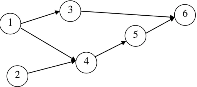
FIGURE ‎2.1PRECEDENCE GRAPH ... 10

FIGURE ‎2.2IMBALANCE FOR ONE STATION, VARIABLE TASK DURATIONS DUE TO VARIANT [16] ... 11

FIGURE ‎2.3 ASSEMBLY LINE MODELS [21] ... 13

FIGURE ‎2.4 A SIMPLE U-SHAPE ASSEMBLY LINE [22] ... 13

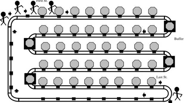
FIGURE ‎2.5LINEAR WALKING WORKER ASSEMBLY LINE [7] ... 26

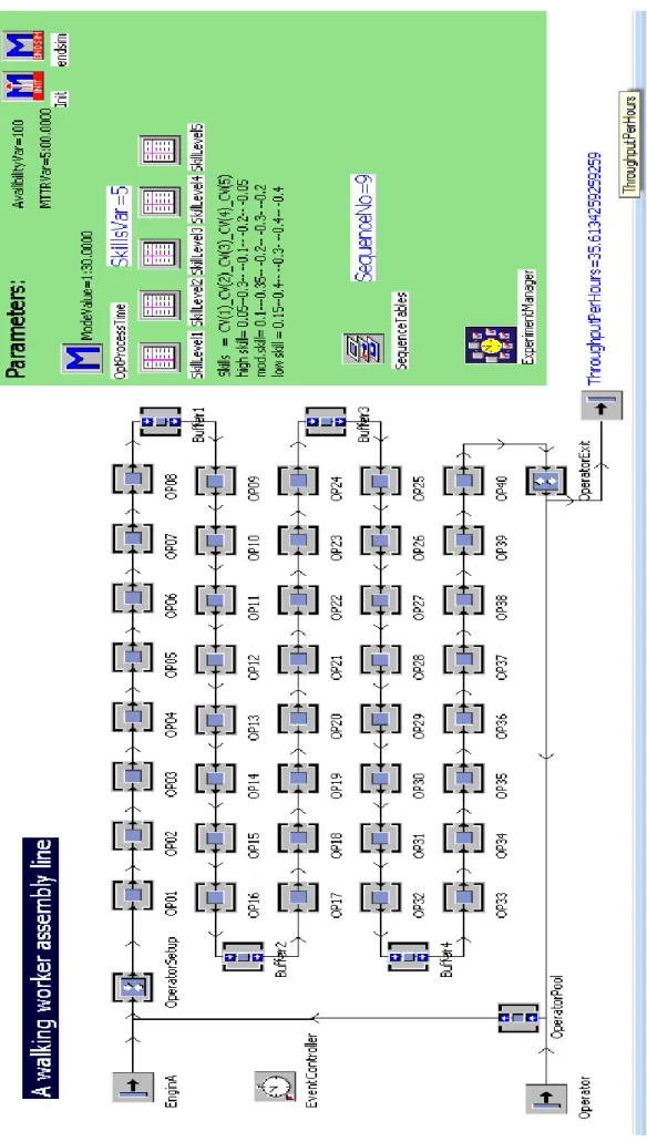
FIGURE ‎4.1 THE WALKING WORKER ASSEMBLY LINE CASE STUDY SCHEME ... 37

FIGURE ‎4.2SIMULATION OF THE MAIN MODEL USING THE PLANT SIMULATION SOFTWARE ... 40

FIGURE ‎4.3TEN REPLICATION AVERAGE FOR THROUGHPUT PER HOUR ... 43

FIGURE ‎4.4MOVING AVERAGE FOR TEN REPLICATIONS FOR THROUGHPUT PER HOUR AND WARM UP PERIOD ... 43

FIGURE ‎5.1THE RESULT FOR CV(5)(MEAN AND CONFIDENCE INTERVAL) ... 46

FIGURE ‎5.2SCHEME OF PATTERN P10, REPETITION OF THE PATTERN WITH RETURNING WORKERS TO THE BEGINNING OF THE LINE. ... 49

FIGURE ‎5.3THE COMPARISON OF WEIBULL AND TRIANGULAR DISTRIBUTIONS AT THE SAME CV LEVEL. ... 52

FIGURE ‎5.4LOW SKILL WORKER REDUCTION COMPARED WITH P2. ... 54

List of Tables

TABLE ‎2.1VERSIONS OF SALBP[25] ... 16

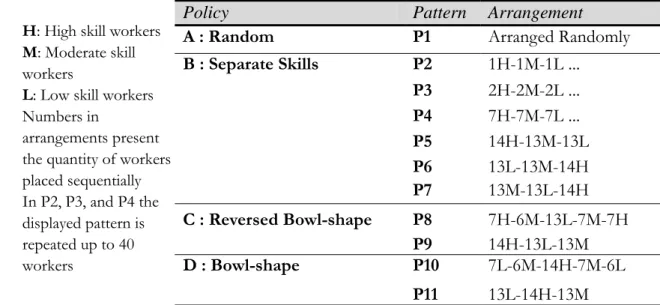
TABLE ‎4.1CONSIDERED ARRANGEMENT OF WORKERS ... 41

TABLE ‎4.2CV(1) TO CV(5): TRIANGULAR DISTRIBUTION AND CV(6) TO CV(8):WEIBULL DISTRIBUTION ... 42

TABLE ‎4.3 CALCULATION OF STANDARD ERROR IN REPLICATION ANALYSIS ... 44

TABLE ‎4.4SIMULATION RESULTS CONSIDERING DIFFERENT NUMBERS OF HIGH AND LOW SKILL WORKERS WITH AND WITHOUT A BUFFER ... 45

TABLE ‎5.1THE RESULTS OF EXPERIMENTMANAGER FOR 11 PATTERNS AND CV(5) ... 46

TABLE ‎5.2SIMULATION RESULT OF CV(5) IN DESCENDING ORDER.(H.SKILL:0.05,M.SKILL:0.2,L.SKILL:0.4). ... 47

TABLE ‎5.3THE PAIRED-T CONFIDENCE INTERVALS FOR DIFFERENCES BETWEEN RANDOM PATTERNS AND TEN OTHER PATTERNS WITH AN OVERALL CONFIDENCE LEVEL OF 0.95 AND AN INDIVIDUAL CONFIDENCE LEVEL OF (1-0.005). 48 TABLE ‎5.4THE PAIRED-T CONFIDENCE INTERVALS FOR COMPARISONS BETWEEN PATTERN P8 AND PATTERNS P5,P6,P7, P9,P10, AND P11 WITH AN OVERALL CONFIDENCE LEVEL OF (1-0.05) AND AN INDIVIDUAL CONFIDENCE LEVEL OF (1-0.0083). ... 49

TABLE ‎5.5THE COMPARISON OF DIFFERENT CV LEVELS; THE NUMBERS BELOW EACH CV RESPECTIVELY DISPLAY THE VALUE OF THE COEFFICIENT OF VARIATION OF HIGH, MODERATE, AND LOW SKILL WORKERS. ... 51

TABLE ‎5.6THE AVERAGE THROUGHPUT RESULT OF ... 52

TABLE ‎5.7THE RESULTS OF REDUCTION OF WORKERS ON THE THROUGHPUT. ... 53

TABLE ‎5.8UNBALANCED LINE PATTERNS ... 55

1 Introduction

This chapter aims at introducing the motivation behind the current study through presenting a brief theoretical background of the subject followed by industrial/practical incentive. Having a clear sense of the problem, objectives have been presented in the form of research questions. Moreover, the scope of the studied problem has been elaborated and the report structure has been elucidated in the end of the chapter.

1.1 Background

The original motivation to build the assembly lines was cost efficient mass-production of standardized products. However, product requirements and thus the requirements of production systems have intensely changed since the times of Henry Ford. Therefore, new technology and production systems have been developed to make assembly lines available to low volume assembly-to-order and mass-customization systems, which are required by increasing variety of customer needs and demand fluctuation in today’s market. This guarantees a high practical application of assembly line systems in the near future [5]. Moreover, the assembly process of product takes a considerable proportion of the manufacturing processes. The study [6] indicated that approximately 40% of product cost is in the assembly phase.

In response to the rapidly varying conditions of the global market and fierce competition, manufacturing companies have applied highly flexible production tools with the use of automated flexible machinery and cross-trained workers. However, several companies, which invested in highly advanced automation, found that automation solution is not sufficiently flexible due to reducing lot size and increasing product variants, thus they reduced their level of automation again [7]. The investigation [1] illustrated that cross-trained workers with performing multiple or all required jobs can significantly improve output over traditional fixed workers. On the other hand, poor responsiveness, little flexibility in system reconfiguration to meet uncertainty of demand, and low efficiency of traditional assembly lines induced manufacturers to apply cross-trained workers who move along the assembly line and carry out their planned jobs in different stations.

The assembly lines, which applied multi-functional workers, are designed in several forms. However, a novel model that is concerned in this study is called the linear walking workers assembly line and is applied with workers who travel along the line, follow the movement of the products and stop in each workstation to carry out assembly jobs of the products. Each cross-trained worker has to fully assemble the product from beginning to end and this feature differentiates this model from other variants of moving workers. A series of studies from University of Bath in UK (e.g. [2], [8], and [9]) has undertaken the research of this type of assembly line and compared it with the traditional fixed-worker assembly line. The investigations results showed significantly high performance of the linear walking worker assembly line over the fixed-worker assembly line, and pointed out some advantages of using this type of assembly lines such as ease of line balancing, high

tolerance of operation time variation, and adjustability of number of operators to respond demand changes, and so forth.

In practice, significant difference in individual capabilities is observable. While with training and appropriate selection the magnitude of differences can be reduced, it has not been proven that they can be omitted [10]. In addition to the deviation of mean operation times, workers differ in the variability of their operation times [3]. In general, individuals cannot perform a series of task repeatedly in the same rate and the result of this is variation in the task times. This variability is usually showed by coefficient of variation (CV) and can be considerably significant [11]. Studies showed that due to variability on operation times which cause blocking and starving in the stations, balanced lines do not result in the optimum performance, but rather particular arrangements of imbalanced stations are suggested to improve line utilization [12]. Hillier and Boling [4] indicated that with unbalancing a line in a bowl shape, i.e. lower mean processing time in the middle stations, could reach optimal production rate. They called this finding the bowl phenomenon. Afterwards, an enormous amount of research has been undertaken to investigate the unbalanced line in different conditions and with different sources of imbalance. El- Rayah [13] examined the effect of different arrangements of stations on the output rate considering unequal CVs and concluded that best output can be obtained when the lower variability stations are gathered in the middle and the higher at the end of the line (bowl shape arrangement). In addition, he showed that the bowl-shaped unbalanced line, in terms of only CV imbalance, yields a maximum output rate significantly higher than the balanced line. Series of other studies also reached similar results, which are implied in the literature review section, although some could not show improvement over the balanced line when the line length increased. Even though the improvement of bowl phenomenon is only about 1% or 2%, it is still

significant and causes large savings for the company since it can be gained with almost no investment and simply through arranging workers with different skills in a specified pattern [14].

In these series of walking-workers assembly lines studies, the difference between workers’ performance has been considered by assigning diverse mean times and coefficient of variation to operation times [15], [9], and [8]. However, to our best knowledge, no published study in the linear walking-worker field has investigated the effect of different arrangement of workers. Thus, for the sake of this research gap, current work has undertaken the investigation of the effect of different arrangement patterns of workers with varied skill levels on the throughput of the walking worker assembly line.

The original motivation of this work arose due to a suggested study on the conceptual design of a walking-worker assembly line by a local company in the automotive industry. The company has successfully applied the walking-worker assembly systems for several years and intends to develop additional line for new product with a similar system. The observed problem in the existing lines is efficiency loss due to variability of workers’ operation times, caused mainly by their diversity in skills and some minor disruptions. The company’s interest is therefore to investigate the effect of workers’ operation variability on the line output of the respective conceptual model. It is expected that using the conceptual

model, the production managers/engineers can gain insight or knowledge to improve the real assembly lines.

Therefore, this industrial problem has been chosen as an industrial case study to examine the research questions of this investigation.

1.2 Purpose and Research Problem

This study, according to an accomplished literature review, contributes to fill a research gap in the field of linear walking worker and unbalanced assembly lines.

Investigation aims at illustrating the influence of workers’ variability and different patterns of imbalances in output, exploring the possibility of improvement without any investment only by arranging workers with different variability in a specified pattern, and examining the existence of bowl phenomenon in this special type of assembly system. The result of this study will partially fulfill the objectives of the company in the industrial case study.

In the following, the research problem has been broken down into the specific research questions and the research hypotheses.

1.2.1 Research questions

To achieve these goals, the problems have been formulated in the following research questions:

In a linear walking worker assembly line in which workers have different variability:

1. Does the arrangement of workers in any pattern cause a significant improvement in the throughput of the line?

If so, which pattern would yield the highest throughput?

2. Does the variability level (variation in CV size and range) affect the validity/magnitude of the previous problem?

3. How does variation in the number of walking workers influence the throughput of the line?

4. Can unbalancing a line, in terms of CV, cause any significant improvement in the throughput over the balanced line?

1.2.2 Research hypotheses

In order to clarify what we are trying to find in this study and create testable statements, the research hypotheses derived from the above-mentioned research questions as follows:

I. Changing the arrangement of the workers with different operational time variability, e.g. due to different skill levels, will significantly affect the throughput of an assembly line with linear walking workers. II. Related to hypothesis I, it is believed that the effect of different variability levels will be more pronounced with the increasing degree of imbalance.

III. A bowl-shaped unbalancing of a linear walking worker line, in terms of CV, can improve the throughput when compared with a perfectly balanced line.

1.3 Delimitations

Unlike the majority of studies in the field of walking worker assembly line, this study do not compare performance of the liner walking worker assembly line with the fixed worker assembly line.

The studies showed that for improvement of unpaced lines’ performance, three issues should be considered. The position of workers with different operation times, different coefficient of variations, and position and size of buffers along the line [11]. This study only investigates the variation of operation times (CVs) and two other factors considered constant in the model. Furthermore, the availability of operators, stations facilities and machines are considered 100% in the model. However, minor disruptions have been taken into account in the coefficient of variations.

1

Figure 2.1 Precedence Graph

2 Literature Review

In this section, a comprehensive literature review of related work in the area of system analysis of assembly lines is presented. This includes:

2.1 Assembly line system

Assembly work has been applied by human beings since a long time ago. Our ancestors knew how to create useful objects comprised of several parts. However, it was the automotive industry which applied present-day assembly lines for the first time. Henry Ford invented the assembly lines that caused a revolution in the way cars are produced and how much they cost. He was a pioneer in developing a moving belt in the factory. This concept enables workers to build cars one piece at a time instead of one car at a time. Based on the so-called division of labor principle, the production process is broken down into a sequence of stages and workers are allocated to specific stages. This gives workers the opportunity to be specialized in one specific job rather than being responsible for a number of tasks [16].

In this part, the basic concepts of assembly lines are described according to [16]. These terms are used widely throughout the literature review part and the rest of report.

Assembly: The practice of fitting different parts together to create the final

product is called the assembly process. Parts by themselves can be comprised of various components and consequently sub-assemblies.

Work in process (WIP): The unfinished units of a product are called work in

process, abbreviated as WIP.

Assembly Line (AL): Flow line production system which consists of number of

stations (n) which are set up along a conveyor system.

Task: The individual part of the total work in an assembly process which

cannot be split into minor work elements without necessary additional work. Task

process time is an essential time that a task needs to be performed.

Precedence Constraints: Technological restrictions, which determine the

order of tasks performance. For illustrating the relationship between tasks, a

precedence graph is a useful tool. The nodes represent tasks and the arrows present

precedence connection. Figure 2.1 shows an example of a six task-assembly process.

Cycle Time (C): Time interval between the exits of two consecutive products

from the line. It represents the maximum amount of work performed by each station. Two types of cycle times can be considered: predetermined cycle time,

desired C, which is required usually by the planning department, on the other hand, effective C or actual C that is based on line performance.

Capacity Supply (CS): The total time available to assemble every product is

defined as CS= nC. The CS can be equal to or greater than the sum of all task process times.

Work Content (WC): The sum of all task process times (Ti). (WC= ∑ Ti)

Station Time: The work content of a station is called station load and total

process time as Station Time.

Imbalance: The measured difference between the Cycle Time and the Station

Time is called Imbalance and when ALs is multi-product, this difference is measured for a given variant on each station (Figure 2.2).

Line Efficiency (E): Measures the capacity utilization of the line and is calculated by E=WC/CS.

Station Idle Time: The difference between the cycle time and the station time

when it is positive is called idle time.

Balance delay: The sum of all station idle times is called delay time or balance

delay and calculated by I=CS-WC.

Throughput Time: Represents the average time between the start of the first

work-piece process and the end of the last finished product process, in other words it is the average process time of a final product in the line.

2.2 Assembly line problems and classification

2.2.1 Problems

With the development of industrial engineering, some multidisciplinary analysis techniques such as time and motion study and analysis of human performance have been introduced to the industry. On the other hand, with increasing complexity in production, line efficiency turns into a significant problem so that increasing efficiency becomes the main purpose of assembly systems. In order to reach high efficiency, developed analysis techniques with a structural approach should be applied in the designing stage of assembly lines [17].

Variant Imbalance for one variant Cycle Time

Figure 2.2 Imbalance for one station, variable task

Assembly line design entails the design of products, processes and plant layout before the construction of the line. Based on classical design for assembly rules and considering precedence constraints between tasks, considerations related to product take into account in line designing. Assembly techniques and modes (manual, automatic) for each task are determined by operating modes and the technique module and assigning tasks to the stations and location of stations and resources in the factory are decided by the line layout module [16].

The line layout problem is comprised of the logical and physical layout. The

logical layout involves assigning tasks to the stations along the line, whereas the physical layout determines the placement of stations, conveyer, buffers, resources,

etc. on the shop floor. In turn, logical line layout consists of assembly line balancing and resource planning problems [16].

Line balancing problem is allocating tasks to an ordered sequence of stations in such a way that precedence relations are pleased and one or some performance criteria are optimized (such as minimizing the number of stations or balance delay) [18]. Baybars [19] defines this typical problem: “The assembly line is said to be balanced if total slack (i.e., the sum of the idle times of all the stations along the line) is as low as possible.” In section 2.2.3 the line balancing problem is discussed in greater detail.

Operations in assembly lines (usually small-sized products) can be performed either manually or automatically. These kinds of assembly lines are called hybrid

assembly lines. In such systems, the design problem decides which resources

(required equipment to complete the operations) to choose and which tasks to allocate to each resource such that production requirements are satisfied and cost minimized.

2.2.2 Classification

In the literature, different classifications for assembly line problems are suggested. This section presents the main categories.

 Assembly line Models

In companies, based on demand of different products, the appropriate plan of production is developed. Thus, assembly lines according to production plan follow three approaches: single model assembly line, mixed model assembly line, multi-model (batch production) assembly line [16], [20], and [18].

Single product assembly line: It is used for producing only one type of product. If

we do not consider the dynamic character of the system, the workload of all stations is constant over time (Figure 2.2.2.1). It is better to use this type of assembly line when the demand of a product is constant, the product must be delivered quickly, or has a different structure from other products and the setup time is considerably long [16]. When the setup times and variations in operating times are not significant, the line which assembles more than one type of product can be treated as single model [20].

Mixed-production assembly line: In these types of assembly lines, the variety of

product is more than one. It is typically a family of products, which is a set of distinguished products (variants) usually with a similar function, and different product attributes (customizable attributes which are referred as options). A family of cars with diverse options (sunroof, ABS, etc.) is a typical example

(Figure 2.2.2.2). In this model, setup times between variants should be reduced significantly enough to be ignored [16]. Balancing the mixed-model assembly line is usually converted to the single- model case through the use of a joint precedence graph. This method with calculating the average process times of different variants in regard to their occurrence forms a unique precedence graph [20].

Multi-model or batch production lines: This model is used when multiple different

products or a family of products with significant differences in production processes are to be assembled in the same line. Thus, for declining extra costs and set up times, products are assembled in batches (Figure 2.3). This requires solving lot-sizing and scheduling problems in addition to the balancing problem [16], [20].

Figure 2.3 assembly line models [21]

 Line configuration:

In design of assembly lines, several configurations of stations are possible. Initial product analysis and form of plant site are the main factors that are taken into account in line layout decision.

Serial lines: in this configuration, the single stations are settled in a straight line

along flow of line [16].

U-shaped lines: recently because of applying just-in-time (JIT) principles in

production, U-shaped layout is preferred to traditional serial line. In this type of line, operators are located in the center of U and in case of hybrid lines; a multi-function worker is responsible to multiple machines and operates on each of them once in one cycle time. Figure 2.4 shows a simple U-shape line in which tasks are assigned to stations, but one irregular station is observable in this line which is different in task grouping from other stations (station 1) [22]. These types of stations which are called crossover stations include tasks located on different parts of the production line and operators travel crossover and return distance to

move between tasks. Station 1 consists of task 1 in beginning of the line and task 11 at the end [23]. U-lines have several important advantages over straight lines, which include: better visibility and communications because of the close vicinity of workers to each other, workers multi-tasking, better flexibility for output rate changes, less stations requirement since there are more possibilities for grouping tasks into stations [22].

Multi-U lines : Miltenburg in his work [23] introduced Multi-U lines as a

developed form of U-lines. This line is combined of n-U shape lines in which adjacent U-lines share an identical station. These stations which are called multiline

stations include tasks from two neighbor U-lines. Balancing methodologies for

these types of assembly lines are disscussed in [22] and [23].

Parallel stations: when the task times in stations exceed cycle time, a common

solution is to build stations with parallel posts where performance of an identical set of tasks is assigned to two or more workers. In this way the average task times reduce proporptionally to the number of workers in the station [16].

Parallel lines: when the demand is high enough, compensation is possible due to

duplication of the entire line. The advantage of these lines is shortening the assembly line and also, in case of failure in one station, other lines continue to run [16].

 Variability of tasks process times

The execution times of tasks can vary in time. The variance can be small in simple tasks or large due to the complexity and unreliability of tasks. This phenomenon is considered in assembly line literature as below:

Deterministic or static time: In reality only advanced machines and robots can work

permanently at a constant speed which makes zero process time variance possible. In the case of manual assembly lines, this might be possible with highly motivated and skilled workers.

Stochastic time: generally, tasks process times have variance and follow a known

distribution function (which might be unknown). Significant variations are usually observable in manual tasks. Non-qualified operators, lack of motivation and training of employees can be the main source of high variance in task times. However, automated lines are also subject to variability, and its source might be a machine breakdown or even defaults of machinery [16], [5]. This subject is discussed more in section 2.3.

Dynamic time: when process times have dynamic variation it should be

considered in balancing problems [20]. This variation can be a systematic reduction due to the learning effects of operators or sequential improvements of the production process [16], [5].

 Line control

Paced lines: in this assembly line system, the given cycle time restricts task

process times of all stations. The pace of line is controlled by: 1) continuously advancing material handling devices such as conveyor belts, which compel workers to finish their tasks before work piece leaves the perspective station. 2) so called intermittent transport systems where the workpiece stops in each station according to a given time. In the continuous system, line balance determines the station length. Once the length of the station (multiplied by the movement rate of the line) goes beyond the cycle time, the extra time emerges which might be used

as compensation for task time deviation in either mixed-model production or the stochastic model.

Unpaced asynchronous line: unlike the paced line in which workpieces have to

spend given times at stations; in unpaced lines, parts are transferred whenever the tasks processes are accomplished. The passing workpieces, after being processed to the following station, distinguish two types of unpaced lines; synchronous when parts transfer simultaneously and asynchronous when each station decides to transfer individually. In the asynchronous mode, workpieces move to other stations (if not blocked by another workpiece) as soon as all required operations have been completed. Then new workpieces enter the stations unless the preceding station cannot deliver. In order to minimize waiting time, a WIP buffer is established between stations. Thus, in unpaced asynchronous systems, there are three interdependent problem which are (1) determining a line balance (2) allocating buffer storage, (3) estimating throughput (depending on the known distribution function of realized task times).

Unpaced synchronous line: all stations wait for the slowest station to finish its

operations and then wokpieces are transferred simultaneously. In the case of deterministic task times, synchronous lines will be the same as paced lines with intermittent transport and cycle times will be equal to the slowest station. These kinds of lines have advantages to paced lines when tasks times have variations. When variation causes fast completion of operations, workpieces can transfer to other stations without waiting any fixed time; therefore synchronous lines can promise higher output than pace lines [20].

2.2.3 Line balancing problem

On account of the high practical significance, a large proportion of the literature is assigned to assembly line balancing (ALB). In general, the line balancing problem consists of academic works focused on the core problem of the configuration, which is the assignment of tasks to stations, since the first mathematical modeling of ALB by Salveson [24]. Due to the several simplifying assumptions which form the foundation of this basic problem, this field of research is labeled as simple assembly line balancing (SALB) in most literatures [5]. The majority of researchers in the ALB field have devoted their work to simple assembly line balancing problem (SALBP) modeling and solving [25]. According to [5] limiting or simplifying assumptions of classical SALB problem are:

“(1) Mass-production of one homogeneous product

(2) All tasks are processed in a predetermined mode (no processing alternatives exist)

(3) Paced line with a fixed common cycle time according to a desired output quantity

(4) The line is considered to be serial with no feeder lines or parallel elements (5) The processing sequence of tasks is subject to precedence restrictions (6) Deterministic (and integral) task times

(7) No assignment restrictions of tasks besides precedence constraints (8) A task cannot be split among two or more stations

Any form of ALB problem intends to find a feasible line balance (allocation of each task to a station in a way that precedence restrictions and other constraints are satisfied) [20]. Nevertheless, different

versions of the SALB problem can be distinguished by varying the objectives (Table 2.1). SALBP-F is a feasibility problem, which looks for the existence of feasible line balance for a given combination of n (number of stations) and c (cycle time). SALBP-1, for a given fixed cycle time c, minimizes the sum of station idle times or equivalently minimizes the number of opened stations. On the other hand, SALBP-2 minimizes the cycle time c (or maximizes the production rate) when the number of stations (n) is given, which results in minimum idle times. SALBP-E is the most common version among these problems. When both the number of stations and the cycle time are changeable, efficiency of line is used to define the quality of a balance. Therefore, the problem consists of maximizing the line efficiency thereby simultaneously minimizing c and n by considering their interrelationship [5], [25]. In addition, a secondary objective for complementing the versions of SALBP is mentioned in the Becker and Scholl study [20], which consists of smoothing station loads, i.e., equalizing the station times. For instance, minimizing the smoothness index SX = √ ∑(C-STi)2 for i=1 to n (No. stations) may be one,

if the combination (n, c) is optimal with respect to line efficiency.

In this part, a simple line balancing method has been described. It is based on the two constraints, precedence requirement and cycle time. The fixed cycle time restriction (paced line) refers to the maximum allowed time that a product can spend at each workstation to meet the required production rate. The method follows below in concise steps (term definitions are described in section 2.1):

1. Prepare precedence diagram 2. Calculate desired cycle time (Cd):

Cd= available production time/desired output

3. Compute the theoretical minimum number of workstation (N): N= ∑all task times (Ti)/ Cd

4. Group tasks into stations with considering cycle time and precedence constraints

5. Compute the actual cycle time (Ca) and real number of stations (n) for arranged group; and then the efficiency of the line (E):

E= ∑ all task times (Ti)/ nCa

6. Determine whether acceptable efficiency level or theoretical minimum number of workstations has been reached. If not, go back to step four [23]. The balancing of real-world assembly lines requires modification in assumptions of SALBP [21]. The line can be mixed or multi-product; can have parallel stations or parallel subassembly lines; can have stochastic task times; and many other characteristics that are not seen in the SALBP. Baybars [19] explains these extended problems as following:

“Whether the goal is to minimize total slack or to minimize the number of the stations along the line, these problems (which created by relaxing one or any

Table 2.1Versions of SALBP [25]

No. of station (n) Cycle time (c)

Given Minimize Given SALBP-F SALBP-2 Minimize SALBP-1 SALBP-E

combination of the SALBP assumptions) will be referred to as the general assembly line balancing problem (GALBP). Thus, GALBP is a generalization of SALBP-1 and SALBP-2.”

A summarized classification scheme is presented in [20], which illustrates the work of Boysen et al. [5]. It has briefly characterized a specific assembly system with all possible relevant extensions by a tuple. This scheme, which is provided in appendix 1, and respective studies [5] and [20] are valuable references either to find an appropriate accomplished study, which can be applied to solve real-world problems or to show research gaps in the field of assembly line systems. Plenty of exact and approximated methods are developed for solving SALBP and GALBP, which their discussion is not in the scope of this work. A recent survey of Scholl and Becker [25] presents a respectable review of developed exact and heuristic methods for SALBPs; on the other hand, the studies [20], [21], and [5] are appreciated references for GALBPs.

Once the size of our problem is significant enough, the balancing of line by hand is a cumbersome job. Therefore, software packages have been developed to balance these kinds of problems quickly. For instance, we can use IBM’s COMSOAL (Computer Method for Sequencing Operations for Assembly Lines) and GE’s ASYBL (Assembly Line Configuration Program). These commercial programs use different heuristics algorithms to balance the line to reach acceptable levels of efficiency. They cannot guarantee optimal solutions [23].

2.3 Variability in assembly lines

2.3.1 Introduction to Variability

In [26] variability has been formally defined as “the quality of nonuniformity of a class of entities.” In manufacturing systems, this nonuniformity emerges in the form of various attributes such as physical dimension, process time, machine failure/repair time, material hardness, setup time, and so on. Variation has been classified into controllable variation and random variation. Controllable variation is the outcome of decisions. For instance, when variant products are produced, the variability will be in the product attributes like their manufacturing time or their dimension. On the other hand, random variation is derived from some events which are not under our immediate control. For example, the time between customers’ demands are not under our control, therefore we should expect to have fluctuation in workstation loads. Similarly, the time that a machine might fail is not known and consequently cannot be predicted or controlled, thus, any kind of outage increases the variability of effective process times in a random manner. In this research, random variation is under study.

There are two basic views about the nature of randomness that are interesting to state here. Hopp and Spearman [26] named apparent and true randomness. In apparent randomness, the only reason that systems appear to act randomly is lack of (or imperfect) information. The premise of this view is that in the case of knowing all the laws of physics and having a complete description of the universe, then in theory, all the details of its evolution are predictable with certainty. Therefore, increasing our information about the process will decrease randomness, and thereby variability. In contrast true randomness, while rejecting

1_{These two premises, as two schools of thought in physics, were among highest striking subjects in early}

20th century. Einstein was defender of first view (incomplete knowledge) and Bohr and others support second view (random universe). Proponents of first view, especially philosophers, criticize the opposite interpretation due to apparent violation of cause-and-effect principle. In return, the followers of the second view point to more fundamental quantities (that are not influenced by randomness: quantum

numbers) as a description to the criticized violation.

the previous premise, believes that processes are truly random. In this notion, the universe actually behaves randomly therefore having a complete description of the universe and the laws of physics would not be enough to foretell the future.1

Regardless of types of randomness, the influences are similar. Many aspects of life are inherently unpredictable and manufacturing management is one of them. However, this does not mean that we should abandon managing and controlling processes, instead we only need to find robust policies. A robust policy provides a work that is well most of the time. It is not optimal but usually relatively good. On the other hand, the optimal policy is the best policy for a specific set of circumstances. It may work extremely well for the designed situation but lead to poor results in many others. However, companies tend to spend a huge amount of money for advanced tools to optimize processes that are inherently random. It would not be an astonishment to get a frequently bad result from these tools since the real inputs are random [26].

Hopp and Spearman [26] believe in a stronger tool for managing which is called

probabilistic intuition. This beside the appropriate robust policy will improve the

performance of enterprises despite the existence of variability. Intuition plays an important role in our everyday life. For example in driving, we slow down our speeds in turns without knowing about complicated automobile physics and it is based on our developed intuition after some time driving. In most cases where what we judge is based on the mean of the random variables, our intuition works well. For instance, when we speed up the bottleneck station, we expect to have better performance. This intuition responds well as long as the variation in the mean quantity is large comparative to the randomness involved.

When the consideration is quantities involving the variance of random variables, our intuition seems to be less practical. For instance, when there is an option to choose between short, frequent machine failure and long, infrequent ones (less disruptive ones). These kinds of situations where variability is involved require much more subtle intuition than when we make decisions based on the mean changes (throughput improvement by raising bottleneck speed) [26].

The above assertions mark the fact that variability studies can support decision maker more than similar studies that consider mean time. This fact emphasizes the importance of this study, which considers the effects of variability (not mean variation) on the assembly line throughput.

To study variability we need to quantify it. This is possible with standard measures from statistics, such as variance and standard deviation. However, these two measures do not appropriately indicate the level of variability when a comparison is supposed to be drawn. Thus, we use a reasonable relative measure of the variability of a random variable, which is called the coefficient of variation (CV), and it results from the division of the standard deviation by the mean. In the book Factory Physics [26], three classes of variability based on the coefficient of variation are considered: low variability when the CV is less than 0.75, moderate variability when the CV is between 0.75 and 1.33, and high variability when the

CV is greater than 1.33. In manufacturing, high variability can occur when we consider the available outages in process times.

The most common sources of variability in production systems are: natural variability, random outages, setups, operator availability, and rework. In the following, some of these causes are described:

Natural variability: it is the variability inherent in natural process time and

consists of minor fluctuations caused by differences in operators, machines, and materials. It does not include random downtimes, setups or any other external effects. Due to the involvement of operators in a majority of these unidentified sources of variability, more natural variability exists in manual lines than in automated ones. In most systems, the variability in the natural process times is low. In other words, the CV is less than 0.75.

In practice, several detractors influence workstations, which can include machine downtimes, setups, operator unavailabilityand so forth. These detractors inflate both the mean and the standard deviation of process times, which provide a way to quantify their effects [26].

Outages: outages can be considered in two groups, Preemptive and Nonpreemptive outages. Preemptive outages, which mainly refer to breakdowns, occur whether we

want them or not for example in the middle of job. The other probable examples for this group can be power outages, emergency calling away of operators, and running out of consumables e.g. oil for machines. Since these detractors have a similar influence on the behavior of production systems, they can be combined together and treated as machine breakdowns. This allows one to compute unique measurements for analyzing this type of variability. The measurements that are privileged in a machine reliability analysis are MTTF, MTTR, and Availability. MTTF is mean time to failure and determines the frequency of downtimes, MTTR or mean time to repair indicates average time of repair (or getting back to uptime), and Availability is the long-term fraction of time that a machine is not down for repair. The relation between availability (A) and the two previous measurements is according to the following equation:

A = MTTF / (MTTF+MTTR)

Nonpreemptive outages include downtimes that take place unavoidably, but during the occurrence are regularly under control. For instance, when a tool starts to become dull and needs to be replaced. In similar situations, we can stop production after finishing the current piece or job. Another common example from this group is process changeover or setup that is more under control, since we can decide how many to make before changing. Nonpreemptive outages could cover preventive maintenance, breaks, operator meetings, and such events. These outages need different treatment than preemptive outages and since the most common nonpreemptive outage is setup, we can combine all other downtimes from this group and cover them under this term [26].

2.3.2 Variability in Task Process Time

As we mentioned in section 2.2, one of the SALBP variants is formed by considering stochastic task process times. The variability discussion in the previous section by describing different sources of variability in manufacturing systems illustrated that assuming deterministic task time is far from reality.

Therefore, considerable amount of research focuses on assembly lines with stochastic task times and the problem of assigning these task times in workstations.

Moodie and Young [27]were among the first people who considered the stochastic task times in detail and presented a procedure for assigning tasks to stations [28]. In this regard, there is great amount of literature which investigates different methods to distribute stochastic tasks among stations to reach ideal situations. Paced assembly lines, since they are not associated with this research, will not be discussed further in this report and the survey [21] is recommended instead as good reference with the outlined accomplished studies.

In deterministic systems, it is apparent that the ideal line is one with a perfect balance in which workloads of stations are equal and idle time is zero. However, this is not true for stochastic cases. It is difficult to define what a proper task assignment is when there is variability in process times [28]. For instance, Kottas and Lau [28], considering incompletion cost (in paced lines), presented a desirable pattern which instead of equal load of work (balanced line), the workload of stations tends to increase as one moves toward the end of the line (more idle time in early stations).

Due to the prevalence of unpaced assembly/production lines in today’s industry, huge amounts of investigation focus on improving the efficiency of these lines. [29] takes into account two issues which are effective for the efficiency of production lines, the assigning of tasks to the workstations and the allocation of buffer storage space between workstations. Accordingly, the latest investigation [11] by McNamara et al. has considered stated influencers based on worker approach (discussed in section 2.4). First, the differences in average operation times of operators make the allocation of operators along the line a significant consideration. Further, since in general individuals cannot perform a series of tasks repeatedly at the same rate, variation in the task times operated by workers can be considerably significant; thus, the positioning of operators with a different CV is another consideration. Other factors are the buffer size and placement. Theoretically even allocation of intersection buffers yields to the best result. Nevertheless, due to some technical restrictions this is not possible always, therefore buffer allocation turns into an influencer. Finally, the line length and total buffer space of line are mentioned as the last influencers on the performance of production lines.

Researchers have investigated the effect of these factors individually and as a combination of them on the efficiency of lines. In this research, since only variation in the CV of process times is considered, the buffer size and allocation are not included in the following literature review and just a brief time is taken for presenting mean imbalance.

Similar to paced lines with stochastic task times, the fact that unpaced production or assembly lines are perfectly balanced does not guarantee maximum output rate of the line. This is due to variability on operation times and limitation of interstage storage capacities, which cause blocking and starving in the stations [12]. Blocking and starving situations have been explained in [3]: “when a station temporarily performs its task faster than a succeeding station it will fill its output buffer and thus be blocked and when a station temporarily performance its task faster than a preceding station, it will deplete its input buffer and thus be starved.”

Both starving and blocking cause delays in the production and consequently deterioration in output rate. Evidently, the probability of occurrence of these two increase with the growing operation time’s variability.

According to the assumption that perfectly balanced lines always produce higher output than other unbalanced equivalents, the majority of studies had considered only perfectly balanced lines. However, a number of researchers tried to test this assumption and suggested different arrangements as the optimal design. Makino [30] tests unequal service rates in the three-station queuing system with exponential distribution and no interstage buffer and found that assigning a lower process time to the middle of the queue improves the efficiency of systems. A number of other authors also suggested different patterns for improving line utilization. However, extended work was accomplished by Hillier and Boling [4]. They investigated and verified Makino’s work. They found that with assigning a lower mean service time to the middle station of a three-station production line (exponential distribution) could obtain the optimal production rate [12]. They called this finding bowl phenomenon, because the pattern of this optimal workload assigned to each station (adjustment in mean times achieved by loading works in stations) should be less in the interior stations than that closer to the beginning and end, and this is similar to the bowl shape [29].

The study [31] explicates the reason behind the bowl phenomenon as: “the effects of blocking and starving of a station are greatest on those stations closest to it. The beginning and end stations of a line affect stations in only one direction, while the middle stations affect stations in both directions. Therefore, assigning les work to the middle stations has a more beneficial effect, since it helps to mitigate the blocking and starving due to service time variability in both directions.”

Since the design of the line to be perfectly balanced is often technically impossible, this finding allows designers deliberately unbalancing a production line in a specific way, to not just prevent drop of output rate rather easily achieve an optimal output higher than the balanced one. This improvement in output rate, though small, gets significant when it can be collected through the whole life of the production line [12].

According to earlier notes, the variability in the process times as a source of imbalance in stations is the main reason of starving and blocking and consequently existence of bowl phenomenon. Nearly all lines have some degree of imbalance, and operation time means and the coefficient of variation (CV) are considered as the main source of this imbalance [3]. Since the Hillier and Boling study [29], a huge number of researchers has tried to test and extend this phenomenon taking into account the effect of either mean or the CV imbalance of operation time on the production rate. In addition, a limited number has also undertaken the combined effect of these two imbalances.

A number of works which took into account the mean imbalance, are as following: Hiller and Boling’s extension work [32]; the El-Rayah study [12] which applied simulation as a method; Hillier and So [14] that extended the 1979-study [32] with increasing line length (up to 9 stations); and their later study [33] on the robustness of bowl phenomenon which showed the superiority of bowl phenomenon over its balanced counterpart in spite of misestimation of the CV or the existence of deviation from bowl allocation.

The effect of unbalancing lines in terms of their CV has been investigated since Anderson’s work [34], which found a possibility to get better results in a 4-station line than a balanced line by arranging stations in a way that begins from a steady station and ends at a variable station. Other initial studies considered an incremental pattern with a high CV towards the end and found a slight increase in output [35]. Discovery of bowl phenomenon encouraged researchers to test the effect of a bowl shaped variability imbalance on the efficiency of a line. Carnall and Wild [36] investigated the efficiency variations of a line induced by different arrangements consisting of constant (automatic machines) and variable stations. They concluded: “Our results support the hypothesis of the existence of a bowl-shaped phenomenon and extend it to the case of changing stage variance rather than mean output rate. It is clear from the results that coefficient of variation and buffer capacity affect the magnitude of the bowl phenomenon.” The achievable improvement with a CV of 0.5 was equal to 4% which is a significant effect whereas, Hillier and Boling [4] got only 1% improvement with mean time unbalancing.

El- Rayah [13] explored two problems: a) the effect of different arrangements of stations on the output rate considering unequal CVs. b) whether unbalancing only the coefficient of variance can enhance output of a balanced line. He considered 3-, 4- and 12-station lines and two levels of variability (CV: 0.15 and 0.3) for the first challenge and three levels for the second problem (CVs: 2, 2.25, and 2.5 under the condition that total variability for all considered arrangements is equal). The results of the experiments supported the bowl phenomenon so that the best result for the first problem came from the arrangement in which the lower variability stations gathered in the middle of line and higher at the end. Having the second problem, the same bowl-shape arrangement yielded to the maximum output rate, significantly higher than balanced line one.

De la Wayhe and Wild [37] could increase the idle time by placing stable stations in the middle of three and four station lines, but they could not reach the same result for a twelve-station line. They consider normal distribution with three levels of variance (relatively stable CV: 0.1; moderately variable CV: 0.2, relatively variable CV: 0.3) and compare a number of arrangements patterns (including bowl shape) with balanced line. However, they could just make the conclusion that using the strategy of separating relatively variable stations with steadier stations might get relatively close results to the balanced line results in any line length. Recently accomplished work [35] also could prove the superiority of the bowl-shaped pattern over balanced line only for short line.

There are several studies in this area which have applied other approaches than simulation such as heuristic approximation or optimization methods, or predictive formula. In [35] a number of these approaches such as [38], [39], and [40] have been listed.

In an investigation of the effects of imbalances on production rate, some literature takes the influence of mean and the CV imbalance into account simultaneously. Rao [41] maintains that the two following patterns are possible optimum arrangements:

a) “Load from the interior stages should be transferred to the exterior ones (bowl phenomenon).” (pattern for mean time imbalance)

b) “Load from the more variable stages should be transferred to less variable ones (variability imbalances).” (pattern for CV imbalance)

He suggested that a) is more significant when the differences in CVs of stations are generally less than 0.5 while b) becomes superior when they go above 0.5.

The [3] investigation demonstrated that the best pattern for decreasing ideal times of line in light of combined imbalance is not similar to when just individual imbalance is considered. The best configuration is resulted when a reverse bowl pattern for mean imbalance and a bowl shaped pattern for CV imbalance are considered.

In addition to the experiments mentioned previously, it is interesting to state a remarkable measurement, which has been conducted by El Rayah [12]. He measured the maximum degree of imbalance, which a considered unbalanced line can bear without decreasing the output rate from the level of its balanced counterpart. This specification of line would intensely support designers in developing efficient production or assembly lines.

2.4 Worker differences

Study [42] states three approaches for modeling variability in task process times. The task approach that considers inherent variability of tasks as a major source of variability, the workload approach which assumes the environment (such as temperature, noise, tooling) as a main source of variability and the last,

worker approach which postulates the workers operating the task as the most

significant source of variability. The authors propose the worker approach because the two earlier approaches ignore the influence of the workers on task process times (or they assume that the same person always performs a job). The task approach models variability by allocating a distribution to each task (mostly assumed normal distribution) and workload approach by setting a distribution (mainly exponential distribution) to the set of tasks in each station. However, the proposed approach models variability in task process times as a function of who performs the task.

Task approach mostly has been used in the studies of stochastic assembly line balancing problems such as [28] and workload approach in the studies of the optimal allocation of imbalances such as [4], [43], and [38] and buffers like [44] and [45] on asynchronous lines.

In this investigation, since operators are a significant source of variability and tasks are performed by different people, the selected viewpoint is worker-based approach.

In planning and designing production systems, usually all workers are assumed equal in their ability to do tasks. Even in stochastic systems when the line is balanced, the task time distributions usually consider the same. Nevertheless, in practice, significant difference in individual capabilities is observable. While, with training and appropriate selection the magnitude of differences can be reduced, it is not proven that they can be omitted [10]. Three categories of slow, medium, and fast, based on workers performance rate, can be considered. Stations with the slowest operators address as bottlenecks and cause delays for other stations and major balancing loss for the line. Besides deviation in mean operation times,

workers differ in the variability of their operation times, which is usually presented by CV [3].

These differences can originate from various sources. The most apparent difference between individuals is in their level of ability. Some people simply perform a task better than others do. This can be due to variances in experience levels, manual dexterity, or just pure discipline. The other easily observed source of distinction is the attitude people have towards their job. Some people prefer responsibility, variety and challenge in their job whereas others want predictability, stability, and a kind of job that lets them leave it behind at the end of the day. In addition to the mentioned observations on workers differences, a distinctive perspective towards life and work can be another source. It causes difference in responses to various forms of motivation. Financial incentives motivate people in different levels and beside that, based on researchers’ findings, different social aspects of work play significant roles in motivating workers [26].

Regardless of the causes of individual differences, the effects of them should be considered in operation management strategies. In a number of literatures, this variance has attracted the researchers’ attention in forms of the labor turnover problem. The numerous costs that are imposed upon high labor turnover rates are the main motivation of this field of studies. Labor turnover cost is logically considered in three types of separation, replacement, and training costs (input cost). However, the significant output cost is neglected here, which addresses the loss of production. It is obvious that this loss results from the difference between production rate of experienced and trained workers and inexperienced and untrained workers [31]. Under the existence of labor turnover, leaving experienced workers are replaced by new or inexperienced workers. Due to the new workers’ learning process, the given task time is longer and more variable than experienced operators’ task times [46]. Influence of increased variability in production rate of one new worker is magnified when the throughput of the entire line is considered (due to starving and blocking of other stations) [31]. Hutchinson et al.’s investigation [31] illustrated not only the effects of this personnel variability, but rather an approach to mitigate the negative effects on the throughput of the assembly lines. They concluded that in a perfectly balanced line, a moderate turnover rate of 6% per month decreased the average annual throughput by at least 12.6% and in higher turnover case (12%), a 16.3% reduction resulted. The approach, which taken by authors to compensate part of this loss, consists of a replacement policy for new workers and unbalancing of workstations’ mean time. The best result, in medium to high turnover rate, obtained by fast-medium-slow replacement policy integrated with a high-medium-low method of imbalance, which improved throughput by 1 to 4%. The higher result right after the best result, which also improved the throughput, is made up of bowl arrangement for replacement policy and interval bowl allocation for the imbalance method.

In the line with the investigation of [31], which searched for a solution to ameliorate the effect of variability introduced by labor turnover, Munoz and Villalobos [46] investigated alternative production methods that under corresponding variability can be better than traditional methods. In fact, the considered approach in this research, to handle variable processing times, was applying dynamic work allocation. In this type of allocation, tasks are not assigned to a specific workstation or operator and the restriction of workers to perform a