Space-time modeling of agricultural landscape variability using AgSimGIS
12
0
0
Full text
(2) Space-Time Modeling of Agricultural Landscape Variability Using AgSimGIS. need to predict hydrologic processes at spatially variable small-scale resolutions. Most agricultural water quality models are based on lumped parameterizations of hillslope to watershed processes, and are thus incapable of providing realistic estimates of spatially variable flow and transport characteristics. Therefore, the estimates of agricultural water quality processes, derived from dominant flow mechanisms, are often inappropriate for making agricultural management and land use planning decisions. This dictates the need for simulating interaction between land areas for environmental hydrologic fluxes, and for a geographically-based system to manage the increased information. In order to address the above problems, the AgSimGIS water quality tool was developed to predict strategic planning scenarios in spatially variable environments across defined agricultural land units. The tool was developed under the Microsoft Visual Studio .NET 2003 environment using the Visual C++ language, and embeds GIS functionality and customization based on programming calls to required ArcGISTM 8.3 ArcObject classes. Specifically, AgSimGIS consists of a multi-functional system that manages and interprets geo-referenced spatial data, and couples a GIS framework to a modified (i.e., quasi-distributed parameter) Root Zone Water Quality Model (RZWQM, Ahuja et al., 2000) for prediction of water quality over a wide range of agricultural management practices and surface processes. The objectives of this paper are to: 1) present a general overview of the RZWQM; and 2) provide a description of AgSimGIS development history, including an overview of the major GIS and modified RZWQM simulation components.. 2. RZWQM DESCRIPTION The RZWQM is a one-dimensional (vertical), process-based agricultural systems model developed in response to increasing needs of scientific support for water quality management. Many of its components have been evaluated, such as water transport (Ahuja et al., 1995), pesticide movement (Ahuja et al., 1995, 1996; Ma et al., 1995, 1996; Azevedo et al., 1997), evapotranspiration (Farahani and Bausch, 1995), subsurface drainage (Johnsen et al., 1995; Singh and Kanwar, 1995; Singh et al., 1996), organic matter/nitrogen cycling (Hansen et al., 1995; Shaffer et al., 2000), and plant growth (Ma et al., 2002). Selected processes are described below and more information is available in the RZWQM Technical Documentation (Ahuja et al., 2000) and the RZWQM User’s Manual (Rojas et al., 2000). 2.1 Water and Chemical Movement Water and chemical transport has been described and tested by Ahuja et al. (1995). A modified Brooks-Corey equation is used to describe hydraulic properties of the soil. Saturated hydraulic conductivity (Ks, cm/h) is calculated from effective porosity φe (Ahuja et al., 1989). Maximum water infiltration rate during rainfall or irrigation events is calculated with a modified Green-Ampt equation (Ahuja et al., 1995). The soil water content is updated at each time interval depending on infiltration rate and water deficiency. Between rainfall or irrigation events, soil moisture is redistributed according to 11.
(3) Ascough et al.. the Richard’s equation. Root water uptake is evaluated using the approach of Nimah and Hanks (1973). For the purpose of solute transport, nitrate (NO3) is assumed to be conservative and has an adsorption constant (Kd) value of zero. To account for physical nonequilibrium, the soil solution is divided into mobile (water in the mesopores of the model) and immobile fractions (water in the micropores). At the end of an infiltration event, water and NO3 in the meso- and micro-pores are allowed to equilibrate and NO3 is transported with water from layer to layer. 2.2 Organic Matter/Nitrogen Cycling (OMNI) In RZWQM, residues (crop stover, manure, and other organics) are partitioned into two pools (fast and slow) based on their C:N ratios. The fraction of residue materials to the fast residue pool (S) is calculated from:. ⎛ 1 1 ⎜⎜ − C (new) C NS S=⎝ n ⎛ 1 1 ⎞ ⎟⎟ ⎜⎜ − ⎝ C NF C NS ⎠. ⎞ ⎟⎟ ⎠. (1). where CN(new) is the C:N ratio of new added materials to the soil, and CNS and CNF are the C:N ratios of slow and fast residue pools, respectively. The fast residue pool has a C:N ratio of 80, and the slow one has a C:N ratio of 8 (modified to account for manure). There are three soil organic matter (OM) or humus pools with C:N ratios of 8 (fast pool), 10 (medium pool), and 12 (slow pool), respectively. The above five pools are dynamically linked together. In addition, there are three living microorganism pools for aerobic heterotrophs (microbial pool 1), autotrophs (microbial pool 2), and facultative heterotrophs (microbial pool 3). Residue and OM pools are subject to a first-order decay with respect to its carbon concentration: r (i ) = kd (i )C (i ). 1< i < 5. (2). where r(i) is the decay rate of pool i (mg-C g-1 d-1), and C(i) is carbon concentration (mg-C g-1 soil). kd(i) is a first-order decay rate coefficient (d-1) and is affected by soil water oxygen concentration, soil pH, ion strength, heterotrophic microbial population, soil temperature, and degree of soil water saturation (Hansen et al., 1995; Shaffer et al., 2000). Minimum microbial populations set in RZWQM are 500, 5000, and 50000 organisms/g soil for microbial pools 1, 2, and 3, respectively. There is no further microbial death if populations are less than their respective minimum populations. The growth of heterotrophs (heterotrophic decomposers and facultative anaerobes) is calculated from OM decay by assuming a fraction of decayed OM components being transferred to microbial biomass. Decayed OM-C has three possible fates: 1) transfer to another OM pool; 2) microbial biomass; and 3) CO2. Autotroph (nitrifier) growth is proportional to nitrification rate. Denitrifier (facultative anaerobes) can also grow under anaerobic conditions and decompose soil residue and soil OM. Death rates for 12.
(4) Space-Time Modeling of Agricultural Landscape Variability Using AgSimGIS. the three microbial populations are calculated as first-order equations with respect to their biomass and the rate coefficients are functions of soil temperature, soil pH, ion strength, soil O2 concentration, total soil C, NO3 concentration, and degree of water saturation. Ammonia volatilization is estimated from the partial pressure gradient of NH3 in the soil and air with due consideration of wind speed and soil depth. 2.3 Evapotranspiration. The RZWQM evapotranspiration (ET) subroutine has been described in detail and evaluated by Farahani and Bausch (1995). Total potential ET is calculated from Shuttleworth and Wallace (1985) and partitioned between evaporation and transpiration based on energy received by the canopy and soil. Evaporation is further divided between bare soil and surface residues. Actual transpiration is conditional on water availability and plant root activity. Actual residue evaporation is equal to potential residue evaporation if the amount of water in the residue surface is equal to or greater than the demand. Actual soil evaporation is equal to potential soil evaporation if the soil conductivity is sufficient to produce the demand at the surface; otherwise it is equal to the maximum amount of water allowed by the soil water flux. If the soil is dry and cannot use the energy to produce evaporative demand, the model assumes 60% of the unused energy is available first to the residue, and then to the plant canopy. If the residue is not able to produce its evaporative demand, 60% of the unused energy is available for the plant canopy. 2.4 Generic Plant Growth Model. This submodel of RZWQM is a generic crop-production model capable of predicting relative plant growth responses to environmental variance and management practices (Ma et al., 2002; Hanson, 2000). It divides a plant into seven phenological growth stages: 1) dormant stage; 2) germinating stage; 3) emergence stage; 4) four-leaf stage; 5) vegetative growth stage; 6) reproductive stage; and 7) senescent stage. Plant development is driven by growing degree-days and plant growth is driven by photosynthesis. A plant requires a certain amount of degree-days before advancing from one phenological stage to another. Photosynthesis is assumed to start when fully functional plant leaves are established at the four-leaf stage. Plants in one growth stage can remain alive in the current stage, pass on to the next stage, or die. Plant population development is estimated from a transition probabilities matrix, which is updated daily according to environmental stresses and phenological growth stage (Hanson, 2000). Nitrogen uptake by plants is passive if the amount of N flow into the plants through water transpiration meets plant N demand, otherwise, active N uptake is required according to Michaelis-Menton equation (Hanson, 2000). Total amount of N taken up by plants is then partitioned into each soil layer in proportion to the root density function. In addition, the model assumes equal availability of NO3 and NH4 to plants.. 13.
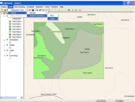
(5) Ascough et al.. 2.5 Agricultural Management Practices. Organic wastes (manure and its beddings) are treated as residues and partitioned into slow and fast residue pools according to Eq. [1], whereas the amount of NH4 in the manure is added into the NH4 pool directly. Surface residues are incorporated into the soil (residue pools) through tillage or biological activities. Beside its effects on residue mass, tillage also reduces soil bulk density, and prevents surface crusting and continuity of microporosity. Soil reconsolidation after rainfall or irrigation is also simulated in the model (Rojas and Ahuja, 2000).. 3. AgSimGIS DESCRIPTION AND DEVELOPMENT AgSimGIS was developed under the Microsoft Visual Studio .NET 2003 environment using the Visual C++ language, and contains GIS functionality and customization based on programming calls to required ArcObject classes.. Figure 1. Main AgSimGIS screen.. Figure 1 shows the main AgSimGIS application screen using the MapControl and TOCControl ArcObjects controls. When embedded in a development environment (e.g., Visual Basic, Visual C++), MapControl provides a window similar to a data view in ArcMap. Land unit map layers are derived via automated intersection of field boundaries (added through the use of drawing tools located on the Main screen toolbar) and USDA-NRCS NASIS soil database information (Fig. 1). The toolbar is a Visual C++ ActiveX control, i.e., it is not based on the ArcObjects ToolbarControl. Additional components of AgSimGIS accessible from the Main screen include Project, Build, Flow Routing, Evaluate, and Scenario (Fig. 1). Project encompasses all data or project management functions including addition of data layers; creating, loading, 14.
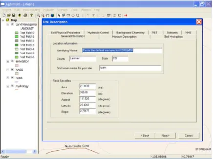
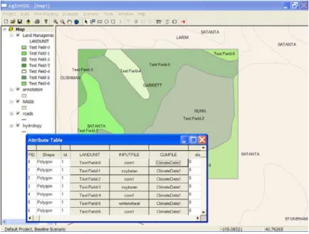
(6) Space-Time Modeling of Agricultural Landscape Variability Using AgSimGIS. saving, and closing projects; and exiting the system. Build invokes core components of the RZWQM98 Windows Interface software application (Rojas et al., 2000) to facilitate creation of the input files necessary to run the RZWQM. Selecting the Build → Inputs → Climate menu item allows the user to input historical daily climate data (e.g., precipitation, temperature, solar radiation, wind speed) or generate daily climate data using the USDA CLIGEN climate generator tool. Selecting the Build → Inputs → Model Parameters menu item allows the user to input all other necessary parameters required by the RZWQM.. Figure 2. AgSimGIS Site Description screen.. Input parameters are grouped by similar processes or properties (e.g., soil, hydrologic, management) into tabbed dialog controls. All tabbed controls are contained within four different screens representing major input parameter categories: 1) Initial System State, 2) Site Description, 3) Residue Condition, and 4) Management Operations. For example, the Site Description screen is shown in Fig. 2. Site Description inputs related to General Information, Horizon Description, Soil Hydraulics, Soil Physical Properties, Hydraulic Control, Background Chemistry, PET, Nutrients, and NH3 are contained on the tabs within this screen. A rudimentary programming “wizard” guides the user through the screens in proper order and also ensures that values for all necessary input variables are entered. After completion of the Build wizard, the completed input data set may be saved to a user-defined file name. This is a departure from the RZWQM98 Windows Interface software which requires pre-determined file names when creating the input file structure. Input files are attached to a specific land unit using the Assemble Input Files screen as shown in Fig. 3 (accessible through the Flow Routing → Assemble Input Files menu item). The desired climate file is also specified in this screen. Currently, a single climate file must be used for all land units; however, this restriction will be 15.
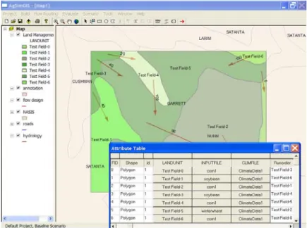
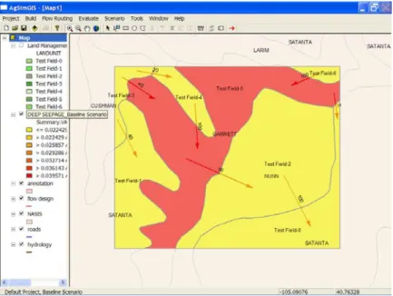
(7) Ascough et al.. removed in future versions of AgSimGIS. After input files have been connected to all land units, the flow routing (i.e., runon/runoff) scheme must be determined. A simple vector-based drawing tool (Fig. 4) is used to identify the runon/runoff pattern across land units. The runoff that a single land unit generates may be partitioned (i.e., flow to) multiple receiving land units. In the example in Fig. 4, 20 percent of the runoff from land unit Test Field-3 flows to Test Field-4, 40 percent to Test Field-5, and 40 percent to Test Field1. The Flow Routing screen is accessible through the Flow Routing → Routing Scheme menu item. Implementation of the AgSimGIS flow routing scheme involved minor modification of the RZWQM source code. Temporary external files for each land unit were created in order to store total runoff produced over the simulation time period. A standalone program, written in C++, uses the information from the Flow Routing screen and creates a simulation control driver that calls the RZWQM in the correct flow routing order for each land unit. The program also partitions and allocates the runoff for those land units receiving runoff fractions.. Figure 3. AgSimGIS Assemble Input Files screen.. Once the flow routing scheme has been completed, the only remaining step before running the modified RZWQM is to select the output variables of interest. RZWQM simulation and output variable control is performed using the Output Setup screen as shown in Fig. 5 (accessible through the Evaluate → Setup Output Variables menu item). The user then selects the Evaluate → Run AgSimGIS menu item to run the modified RZWQM for all land units (using the manually-created routing scheme).. 16.
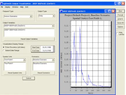
(8) Space-Time Modeling of Agricultural Landscape Variability Using AgSimGIS. Figure 4. AgSimGIS Flow Routing screen.. Figure 5. AgSimGIS Output Setup screen.. After the simulation has been completed, the output variables of interest are extracted (for each land unit) from standard RZWQM ascii output files. Four geodatabases are then created containing temporal (i.e., daily, monthly, yearly) and non-temporal (i.e., summary statistics such as mean, variance, and skew) output data. The temporal databases consist of the land unit name; simulation day, month and year; and values for all selected output variables. The non-temporal database consists of the land unit name and summary statistics. The output data in the geodatabases may then be accessed from the Output Visualization screen (Figs. 6-9).. 17.
(9) Ascough et al.. Figure 6. AgSimGIS Output Visualization screen for temporal data.. This screen controls the output type (i.e., daily, monthly, yearly, summary), the output variables, the number of land units, and the number of scenarios. The appropriate graph type is then displayed. For temporal data, is this normally a standard line graph (Fig. 6); for summary data with a small number of land units, a bar graph is commonly displayed (Fig. 7); for summary data with all land units, a color ramp type of graph is typically used (Fig. 8).. Figure 7. AgSimGIS Output Visualization screen for summary data (maximum of three spatial units allowed).. 18.
(10) Space-Time Modeling of Agricultural Landscape Variability Using AgSimGIS. Figure 8. AgSimGIS Output Visualization screen for summary data (all spatial units graphed).. Exact graph types also depend on the overall graph request type (i.e., basic graphing, comparison type graphs, or query type graphs). Fig. 9 is an example of a query type graph where the land units satisfying the query (show all land units with deep seepage over 0.02 cm/day) have been highlighted.. Figure 9. AgSimGIS Output Visualization screen for a query request.. 4. SUMMARY AgSimGIS is a GIS tool for spatial data input/storage, simulation, display; and transfer of information and data between consultants and researchers. 19.
(11) Ascough et al.. It offers a spatial framework for integrating a complex, quasi-distributed parameter water quality model and also provides the increased interface sophistication necessary for distributed modeling. The prototype AgSimGIS explicitly simulates water movement across agricultural landscapes using a simple overland flow routing scheme between land units. Future research will involve application of the system to measured soil-water dynamics in space and time on an undulating agricultural field in eastern Colorado. The hydrology of water movement and availability in the landscape is the dominant factor controlling both dryland crop growth and the transport of agricultural chemicals in this environment. Thus, AgSimGIS may serve as an integrated GIS-modeling tool for addressing agricultural management, production, and chemical fluxes. Acknowledgements. We gratefully acknowledge the programming support from Bruce Vandenberg, Bob Flynn, and John Norman during the development of AgSimGIS. REFERENCES Ahuja, L.R., D.K. Cassel, R.R. Bruce, and B.B. Barnes, 1989: Evaluation of spatial distribution of hydraulic conductivity using effective porosity data. Soil Sci., 148, 404-411. Ahuja, L.R., K.E. Johnsen, and G.C. Heathman, 1995: Macropore transport of a surfaceapplied bromide tracer: Model evaluation and refinement. Soil Sci. Soc. Am. J., 59, 12341241. Ahuja, L.R., Q.L. Ma, K.W. Rojas, J.J. T.I. Boesten, and H.J. Farahani, 1996: A field test of root zone water quality model - pesticide and bromide behavior. Pest. Sci., 48, 101-108. Ahuja, L.R., K.W. Rojas, J.D. Hanson, M.J. Shaffer, and L. Ma (Eds.), 2000: Root Zone Water Quality Model. Water Resources Publications, Englewood, CO. 372 pp. Azevedo, A.S., R.S. Kanwar, P. Singh, L.R. Ahuja, and L.S. Pereira, 1997: Simulating atrazine transport using root zone water quality model for Iowa soil profiles. J. Environ. Qual., 26, 153-164. Farahani, H.J. and W.C. Bausch, 1995: Performance of evapotranspiration models for maizeBare soil to closed canopy. Trans. ASAE, 38, 1049-1059. Hansen, S., M.J. Shaffer, and H.E. Jensen, 1995: Developments in modeling nitrogen transformations in soil. In: P. E. Bacon (Ed.), Nitrogen Fertilization in the Environment. Marcel Dekker, Inc. New York, NY. pp. 83-107. Hanson, J.D., 2000: Generic crop production – Chapter 4. pp. 81-118. In: Ahuja, L.R., K.W. Rojas, J.D. Hanson, M.J. Shaffer, and L. Ma (Eds.), Root Zone Water Quality Model. Water Resources Publications LLC, Englewood, CO. Johnsen, K.E., H.H. Liu, J.H. Dane, L.R. Ahuja, and S.R. Workman, 1995: Simulating fluctuating water tables and tile drainage with a modified root zone water quality model and a new model WAFLOWM. Trans. ASAE, 38, 75-83. Ma, L., D.C. Nielsen, L.R. Ahuja, J.R. Kiniry, J.D. Hanson, and G. Hoogenboom, 2002: An evaluation of RZWQM, CROPGRO, and CERES-maize for responses to water stress in the Central Great Plains of the U.S. pp. 119-148. In: Ahuja, L.R., L. Ma, and T.A. Howell (Eds.), Agricultural System Models in Field Research and Technology Transfer. CRC Press, Boca Raton, FL. 20.
(12) Space-Time Modeling of Agricultural Landscape Variability Using AgSimGIS Ma, Q.L., L.R. Ahuja, K.W. Rojas, V.F. Ferreira, D.G. DeCoursey, 1995: Measured and RZWQM predicted atrazine dissipation and movement in a field soil. Trans. ASAE, 38, 471-479. Ma, Q.L., L.R. Ahuja, R.D. Wauchope, J.G. Benjamin, and B. Burgoa. 1996. Comparison of instantaneous equilibrium and equilibrium-kinetic sorption models for simulating simultaneous leaching and runoff of pesticides. Soil Sci., 161, 646-655. Nimah, M. and R.J. Hanks, 1973: Model for estimating soil-water-plant-atmospheric interrelation: Description and sensitivity. Soil Sci. Soc. Am. J. 37, 522-527. Rojas, K.W. and L.R. Ahuja, 2000: Management practices – Chapter 8. pp. 245-280. In: Ahuja, L.R., K.W. Rojas, J.D. Hanson, M.J. Shaffer, and L. Ma (Eds.), Root Zone Water Quality Model. Water Resources Publications LLC, Englewood, CO. Rojas, K.W., L. Ma, and L.R. Ahuja, 2000: RZWQM98 User Guide, Appendix - Root Zone Water Quality Model. pp. 327-364. In: Ahuja, L.R., K.W. Rojas, J.D. Hanson, M.J. Shaffer, and L. Ma (Eds.), Root Zone Water Quality Model. Water Resources Publications LLC, Englewood, CO. Shaffer, M.J., K.W. Rojas, D.G. DeCoursey, and C.S. Hebson, 2000: Nutrient Chemistry Processes (OMNI) - Chapter 5. pp. 119-144. In: Ahuja, L.R., K.W. Rojas, J.D. Hanson, M.J. Shaffer, and L. Ma (Eds.), Root Zone Water Quality Model. Water Resources Publications LLC, Englewood, CO. Shuttleworth, W.J. and J.S. Wallace, 1985: Evaporation from sparse crops - an energy combination theory. J. Royal Meteorol. Soc., 3, 839-855. Singh, P. and R.S. Kanwar, 1995: Simulating NO3-N transport to subsurface drain flows as affected by tillage under continuous corn using modified RZWQM. Trans. ASAE, 38, 499506. Singh, P., R.S. Kanwar, K.E. Johnsen, and L.R. Ahuja, 1996: Calibrating and evaluating the subsurface drainage component of RZWQM for different tillage systems. J. Environ. Qual., 25, 56-62.. 21.
(13)
Figure
+3
Related documents
A human activities space, as a target space for 3D and depth reconstruction, provides constraints to the design and planning of the active stereo camera system. The sensor
At first, the product-farnily tier clusters the product features to the semantic cornponents that are implernented by the properties of the architectural cornponents of the
As the CHC theory is currently the most contemporary framework of cognitive factors (Schneider and McGrew 2012), it is most appropriate to define spatial ability based on its
Let A be an arbitrary subset of a vector space E and let [A] be the set of all finite linear combinations in
Small scale spatial and temporal variability of microclimate in a fellfield landscape, Marion Island
Mixed Pickle has lower minimum temperatures, higher temperature range during overcast conditions and smaller spatial variability in cold and warm areas than Tafelberg.. Tafelberg
This case is borrowed from ABSINTHE, a current collaboration project with Cetetherm AB, one of the world-leading producers of district heating substations [11]. The
The result is also an extended version of VTK for our stereoscopic display, a C++ library meant to help users to port their program for stereoscopic visualization and some examples
There are three input signals to the subsystem: the supercapacitor voltage, the fuel cell output current and the fuel cell output power; on one branch the fuel cell voltage
