The Model Optimization, Uncertainty, and SEnsitivity analysis
(MOUSE) toolbox: overview and application
James C. Ascough II, Timothy R. Green
USDA-ARS-PA, Agricultural Systems Research Unit, Fort Collins, CO 80526 USA Christian Fischer, Sven Kralisch
Dept. of Geoinformatics, Hydrology and Modelling (DGHM), Friedrich Schiller University Jena, Germany Nathan Lighthart, Olaf David
Depts. of Computer Science & Civil and Environmental Engineering, Colorado State University
Abstract. For several decades, optimization and sensitivity/uncertainty analysis of environmental models has been the subject of extensive research. Although much progress has been made and sophisticated methods developed, the growing complexity of environmental models to represent real-world systems makes it increasingly difficult to fully comprehend model behavior, sensitivities and uncertainties. This presentation provides an overview of the Model Optimization, Uncertainty, and SEnsitivity Analysis (MOUSE) software application, an open-source, Java-based toolbox of visual and numerical analysis components for the evaluation of environmental models. MOUSE is based on the OPTAS model calibration system developed for the Jena Adaptable Modeling System (JAMS) framework, is model-independent, and helps the modeler understand underlying
hypotheses and assumptions regarding model structure, identify and select behavioral model parameterizations, and evaluate model performance and uncertainties. MOUSE offers well-established local and global sensitivity analysis methods, single- and multi-objective optimization algorithms, and uses GLUE methodology to quantify model uncertainty. MOUSE has a robust GUI that: 1) allows the modeler to constrain objective functions for specific time periods or events (e.g., runoff peaks, low flow periods, or hydrograph recession periods); and 2) permits graphical
visualization of the methods described above in addition to access and visualization of numerous tools contained in the Monte Carlo Analysis Toolbox (MCAT) including dotty plots, identifiability plots, and Dynamic Identifiability Analysis (DYNIA). Following a brief system overview, we present a basic application of MOUSE to the HyMod conceptual hydrologic model.
1. Introduction
A consequence of environmental model complexity is that the task of understanding how environmental models work and identifying their sensitivities/uncertainties, etc. becomes progressively difficult. Comprehensive numerical and visual evaluation tools have been developed such as Monte Carlo Analysis Toolbox (MCAT, Wagener and Kollat 2007) and OPTAS (Fischer et al. 2012) to help analyze environmental model input (state, parameter) and output spaces. In general, these tools function as diagnostic aids that can help quantify the identifiability of an environmental model, i.e., the task of identifying a single parameter or a group of parameter sets within a specific model structure as robust (or behavioral) representations of the system under analysis. Assessing environmental model identifiability is important if the model will be used to predict future behavior, i.e., parameter sets should be identified that reflect “realistic” model prediction of changes to (and impacts on) the physical system. While MCAT and OPTAS are useful for exploring model performance, sensitivity/uncertainty, and underlying assumptions regarding model structure, they both rely on additional software platforms to run [i.e., MCAT requires the MATLAB programming environment and OPTAS is only available as part of the Jena Adaptable Modelling System (JAMS) framework]. Therefore, the primary goal of this research study was to convert the tools found in MCAT and OPTAS to open-source,
Java-based visual and numerical analysis components and integrate them within a fully standalone toolbox. This paper provides an overview of the Model Optimization, Uncertainty, and SEnsitivity Analysis (MOUSE) software application, In addition to an overview of MOUSE, a basic application of MOUSE to the HyMod model is presented to further demonstrate the integrated model behavior, optimization, and
sensitivity/uncertainty analysis tools. 2. Mouse Toolbox Overview
The MOUSE toolbox is directly based on the OPTAS model calibration system (housed within the JAMS environmental modeling framework) which in turn contains the MATLAB analysis and visualization functions found in MCAT converted into discrete Java components. MOUSE is model-independent and is a standalone software application, i.e., no additional 3rd party software programs are required to operate the toolbox. MOUSE can be used to analyze the results from Monte-Carlo parameter sampling experiments or from various single- and multiple-objective model optimization methods. A number of techniques are included in the toolbox to investigate the structure, sensitivity, and parameter and output uncertainty of environmental models.
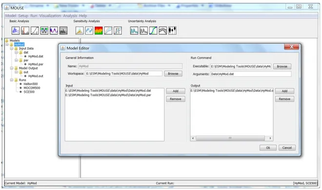
Figure 1. MOUSE Model Editor screen.
The MOUSE main screen featuring the Model Editor window is shown in Figure 1. The Model Editor controls the general model setup including the workspace location, location of the input and output files, and run command information that specifies the location of the model executable file and required arguments. Figure 2 shows the
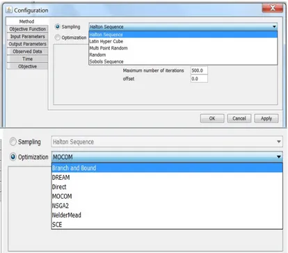
Configuration screen which controls the selection of Monte Carlo sampling and single- and multi-objective optimization techniques, selection of the objective functions (23 objective functions are currently available including Nash-Sutcliffe model efficiency, Index of Agreement d, Root Mean Square Error, Mean Absolute Error, Relative Absolute Error, and Average Volume
Figure 2. Configuration screen showing the Monte Carlo sampling and optimization methods available in
MOUSE.
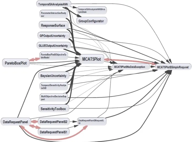
Error), definition of model input and output parameters (including the exact location of the parameters in the input and output files), the location of the observed data file(s), and the simulation start/end dates. Available Monte Carlo sampling techniques include Halton Sequence, Latin Hypercube, Multi-Point Random, Random, and Sobol’ Sequence (Figure 2). Single- and multi-objective optimization techniques currently available in MOUSE include Branch and Bound, DREAM, MOCOM, NSGA-II, Nelder-Mead, and Shuffled Complex Evolution (SCE) (Figure 2). The full suite of available MOUSE tools is shown in Figure 3 and major MOUSE Java classes related to MCAT toolbox implementation are shown in Figure 4.
Figure 3. MOUSE basic analysis, sensitivity analysis, and uncertainty analysis tools.
MOUSE offers well-established local and global sensitivity analysis methods including FAST, Sobol’, and Morris Screening. Most SA methods require an uncorrelated, uniformly distributed, and representative sampling of the parameter space, which is easily generated by drawing as many samples from a uniform probability distribution as needed.
Unfortunately, each method demands distinct sampling properties (e.g., information about partial derivatives) so that a sampling often cannot be reused. Therefore, large
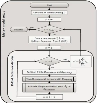
computational effort has to be spent to perform this task multiple times. To overcome this limitation, a single quasi-random sampling is used in MOUSE to generate a meta-model based on an Artificial Neural Network (ANN) which imitates the original model. To setup the meta-model, a multi-step procedure is carried out that first generates an initial sampling (e.g., Halton Sequence), uses the sampling to train the ANN in such a way that it imitates the model response, and then uses a K-fold cross-validation to estimate the agreement between the real model and the meta-model. In case the test fails (i.e., the agreement is not acceptable) additional samples are generated and the procedure is repeated. Otherwise, the information content of the sampling is deemed sufficient to reproduce the characteristics of the original model. The meta-model is now able to dynamically generate samplings with arbitrary properties. The flow chart in Figure 5 summarizes this process. In MOUSE, an ANN consisting of an input layer, one hidden layer, and an output layer, is used. The input layer contains n+1 neurons, which equals the number of input factors plus an additional node to model a constant bias. The hidden layer consists of 0.5(n+1) neurons and the output layer has one neuron. The activation function of the hidden layer is a sigmoid function and that of the output layer is a linear function. Prior to the training process, a linear transformation normalizes the training set. The application uses the Encog Java and .NET Artificial Intelligence Framework (Heaton Research 2014) and the Resilient
Propagation learning rule (Riedmiller and Braun 1993).
Figure 5. Flowchart of the sampling and ANN training process.
3. Mouse Example Application using the HyMod Model 3.1 HyMod model description
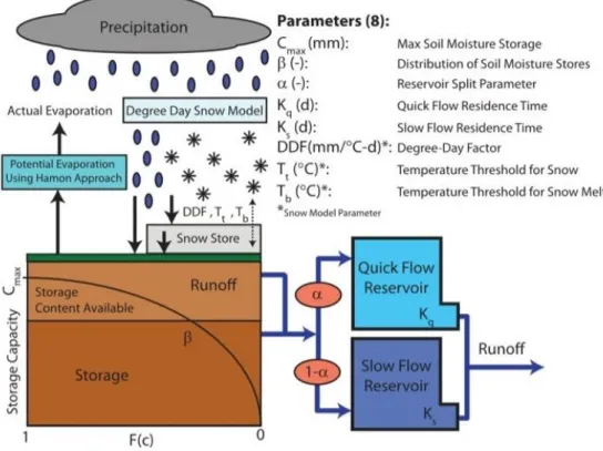
The lumped conceptual hydrologic model HyMod (Boyle et al. 2000; Wagener et al. 2001) is composed of a snow module, soil-moisture accounting module, and a routing module (Figure 6). HyMod uses a simple degree-day method (Bergström 1975) for calculating snowmelt. When the average air temperature for a day falls below the temperature threshold for snow (Tt), snow storage occurs. When the average daily air temperature is above the temperature threshold for snowmelt (Tb), snowmelt occurs at the rate defined by the degree-day factor (DDF). The storage elements of the catchment are distributed according to a probability density function defined by the maximum soil moisture storage, and the distribution of soil moisture stores. The maximum soil moisture storage (Cmax) represents the capacity of the largest soil moisture store, while the shape parameter (β) describes the degree of spatial variability of the stores (Wagener et al. 2004). Evaporation from the soil moisture store occurs at the rate of the potential evaporation estimated using the Hamon approach. Following evaporation, the remaining rainfall and snowmelt are used to fill the soil moisture stores. Excess rainfall is divided in the routing module using a split parameter (α) and then routed through parallel conceptual linear reservoirs meant to simulate the quick and slow flow response of the system. The flow from each streamflow is the addition of the outputs from each of these reservoirs. There are a total of eight parameters that must be calibrated for HyMod as shown in Figure 6 and Table 1.
Figure 6. Schematic of the HyMod conceptual hydrologic model including calibration parameter definitions
(after Kollat et al. 2012).
Table 1. Lower and upper sampling bounds used in MOUSE for the HyMod input parameters.
Parameter
name (unit) Parameter description Lower bound Upper bound Ks (day-1) Slow flow routing tank rate parameter 0.0 0.15
Kq (day-1) Quick flow routing tank rate parameter 0.15 1
DDF(mm
ºC-day-1) Degree-day factor 0 20
Tb (ºC) Base temperature to calculate snowmelt -3.0 3.0
Tt (ºC) Temperature threshold -3.0 3.0
α (unitless) Quick/slow flow split parameter 0 1
β (unitless) Scaled distribution function shape parameter 0 7 Huz (mm) Maximum height of the soil moisture accounting tank (used with β to calculate C
max). 0 2000
3.2 HyMod input data and MOUSE setup
The HyMod model was run under MOUSE using streamflow data for the Guadalupe River Basin in Texas, USA taken from the Model Parameter Estimation Experiment (MOPEX) dataset (Duan et al. 2006). For many of the MOPEX watersheds, the available data range was from 1 January 1948 to 31 December 2003 with occasional gaps. For this example application, we analyze the period 1 October 1961 to 30 September 1972, i.e., 10 years plus a 1-yr warm-up period to remove the effects of initial conditions. The 10-yr period was selected because it contains uninterrupted daily data for the Guadalupe River Basin. Table 1 shows the lower and upper sampling bounds used in MOUSE for the HyMod input parameters as shown in Figure 6.
3.3 MOUSE evaluation
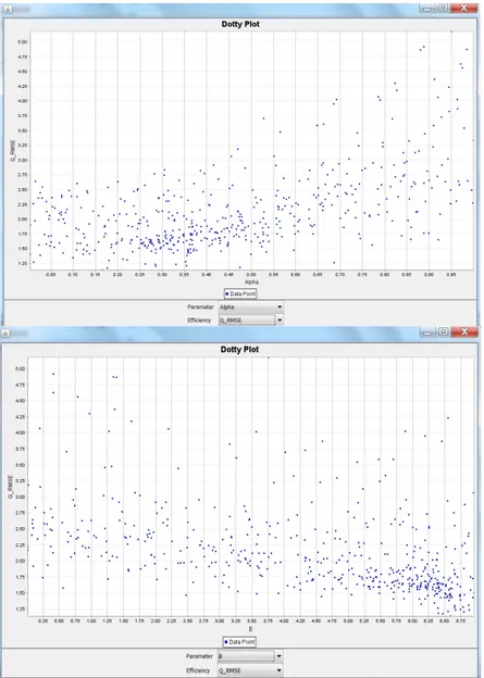
3.3.1 Dotty plots. Dotty plots map model parameter values and their corresponding
objective function values to 1-D points and provide a means of assessing the identifiability of model parameters. Dotty plots of the Root Mean Square Error (RMSE) (streamflow) objective values versus HyMod α and β parameter values resulting from 1000 uniform random samples of the parameter space are shown in Figure 7. In MOUSE, the user is provided with a combo box capable of changing the objective function threshold which is displayed on the dotty plots to aid in providing a visualization which best displays the identifiability of each parameter. In Figure 7, note that in general a range of α and β values result in very similar RMSE objective function values indicating low identifiability in terms of this objective. However, there are two areas for α (between 0.25 and 0.40) and β (between 5.75 and 6.75) where the values are more densely clustered together indicating higher identifiability.
Figure 7. Dotty plots of RMSE vs. HyMod α and β parameter values resulting from 1000 uniform random
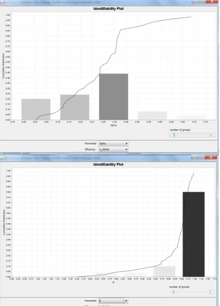
3.3.2 Identifiability plots. Identifiability plots (Figure 8) provide another means of visualizing the identifiability of HyMod α and β model parameters by plotting the cumulative distribution of the top 10% of the parameter population in terms of RMSE objective function values for streamflow. High gradients in the cumulative distribution indicate high identifiability in the top performing model parameters whereas shallower gradients indicate low identifiability. In addition to the cumulative distribution function, the top 10% of the parameter population is divided into user-selected bins of equal size and the gradient of the cumulative distribution is then calculated for each group. These
gradients are plotted as bars on the identifiability plots with shading indicative of gradient. This provides additional visualization functionality as the height and shade of the bars indicate identifiability within the range of each group. In Figure 8, it can be seen that α has the highest identifiability within the range of 0.28-0.40 and β has the highest identifiability within the range of 6.5-7.5.
Figure 8. Identifiability plots of RMSE vs. HyMod α and β parameter values resulting from 1000 uniform
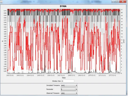
3.3.3 Dynamic Identifiability Analysis (DYNIA). Wagener et al. (2003) introduced the Dynamic Identifiability Analysis (DYNIA) approach which consists of an algorithm based on ideas presented by Beck (2005) and extends components of the GLUE algorithm (Beven and Binley 1992). DYNIA can be used to find informative regions with respect to model parameters, to test model structures (assuming that varying parameter optima indicate structural problems), and to analyze experimental design (Wagener and Kollat 2007). It uses the identifiability measure shown in Figure 8 and applies it in a dynamic fashion using a Monte Carlo based smoothing algorithm. The user must choose a window size to calculate a moving mean of model performance (using the mean absolute error criterion). A different identifiability plot is therefore produced for every time step and a gray color scheme is used to show the variation in the marginal posterior distributions for each parameter. The window size has to be selected with respect to the function of the parameter (temporal length of the region of influence) and the quality of the data (better data allows the use of a smaller window). In Figure 9, the darker gray regions indicate peaks in the distributions, the red line is the 90% confidence limit, and the black
continuous line is the observed streamflow hydrograph. The DYNIA algorithm utilizes the top 10% of all data sets to calculate the distribution at every time step. Figure 9 shows that the information content of the data with respect to the β parameter is highest at values above 6.25. This range is similar to those found for β in the dotty plot (5.75-6.75) and identifiability plot (6.5-7.5) analyses.
Figure 9. DYNIA plot for the HyMod β parameter with a 10-day window period.
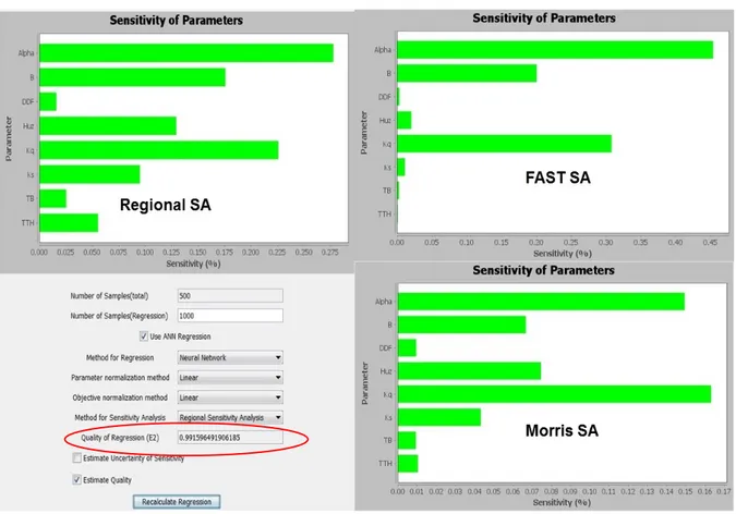
3.3.4 Sensitivity analysis. A sensitivity analysis (SA) was carried out for seven HyMod model parameters (Cmax was calculated using the Huz and β parameters) so that the effect of the parameters on the Nash-Sutcliffe efficiency between the simulated and observed streamflow could be assessed. The ANN was able to accurately imitate the HyMod model as a Nash-Sutcliffe efficiency of more than 0.99 between the original model and the
meta-model (see “Quality of Regression” in Figure 10) was achieved. This estimation is based on a ten-fold cross-validation. The Regional Sensitivity Analysis (RSA), FAST, and Morris methods provide sensitivity indices (linearly normalized to make them comparable) which can be used to create a priority ranking of the input parameters. The resulting
rankings of the three SA methods are not equal; however, the same parameters (α, β, and Kq) are classified as sensitive for all three methods (the Morris method shows the Huz parameter as also being sensitive).
Figure 10. RSA, FAST, and Morris method sensitivity analysis results for HyMod input parameters.
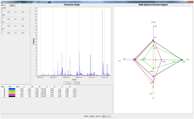
3.3.5 Multi-objective analysis. The multi-objective analysis plot is useful for visualizing trade-offs between different objective functions which often provide conflicting
optimization targets (typically a solution that is best in terms of all objective functions cannot be identified). As a result, a Pareto optimal set of solutions can be identified which are non-dominated with respect to one another (i.e., improved performance in one
objective results in decreased performance in one or more of the remaining objectives). Figure 11 shows multi-objective tradeoffs across different objective functions for HyMod model streamflow evaluation using spider plot (also known as radar plot) visualization. The plot is a diagram in the form of a web that is used to indicate the relative influence of different parameters, or in this case objective functions. Spider plots are effective
visualization tools when there are more than three factors that can influence a result. The factors that have most influence are mainly located on the periphery of the web and the factors that have little influence are located at the center of the web.
Figure 11. Multi-objective tradeoffs across different objective functions for HyMod model streamflow
evaluation using spider plot visualization. 4. Summary and Conclusions
This paper provides an overview of the MOUSE software program, an open-source, Java-based toolbox of visual and numerical analysis components for the evaluation of environmental models. MOUSE is based on the OPTAS model calibration system
developed for the Jena Adaptable Modeling System framework, is model-independent and helps the modeler understand underlying hypotheses and assumptions regarding model structure, identify and select behavioral model parameterizations, and evaluate model performance and uncertainties. The MOUSE toolbox was designed to be applied to evaluate models in a research context in hydrological and environmental studies. MOUSE offers well-established local and global sensitivity analysis methods, single- and multi-objective optimization algorithms, and uses GLUE methodology to quantify model uncertainty. Its simplicity of use and the ease with which model results can be visualized make it an effective tool as illustrated herein with the HyMod application. Further
evaluation algorithms/methods are currently being integrated into the MOUSE toolbox to increase its flexibility in analyzing environmental models.
References
Beck, M.B., 2005: Environmental foresight and structural change. Environ. Modell. & Soft. 20(6), 651-670. Bergström, S., 1975: The development of a snow routine for the HBV-2 model. Nord. Hydrol. 6(2), 73-92. Beven, K.J. and Binley, A.M., 1992: The future of distributed models: model calibration and uncertainty
prediction. Hydrol. Process. 6, 279-298.
Boyle, D.P., Gupta, H.V., and Sorooshian, S., 2000: Toward improved calibration of hydrologic models: Combining the strengths of manual and automatic methods. Water Resour. Res. 36(12), 3663-3674, doi:10.1029/2000WR900207.
Duan, Q. et al., 2006: Model parameter estimation experiment (MOPEX): An overview of science strategy and major results from the second and third workshops. J. Hydrol. 320(1-2), 3-17.
Fischer, C., Kralisch, S., Krause, P., and Flügel, W-A., 2012: An integrated, fast and easily useable software toolbox which allows comparative and complementary application of various parameter sensitivity analysis methods. In: Proc. International Congress on Environ. Modell. & Soft., Sixth Biennial Meeting. Leipzig, Germany.
Heaton Research, 2014: http://www.heatonresearch.com/encog.
Kollat, J.B., Reed, P.M., and Wagener, T., 2012: When are multiobjective calibration trade-offs in hydrologic models meaningful? Water Resour. Res. 48, W03520, doi:10.1029/2011WR011534.
Riedmiller, M. and Braun, H., 1993: A direct adaptive method for faster backpropagation learning: the RPROP algorithm. IEEE International Conference on Neural Networks, Vol. 1, pp. 586-591. doi: 10.1109/ICNN.1993.298623
Wagener, T., Boyle, D.P., Lees, M.J., Wheater, H.S., Gupta, H.V., and Sorooshian, S., 2001: A framework for development and application of hydrological models. Hydrol. Earth Syst. Sci. 5(1), 13-26.
Wagener, T., 2003: Evaluation of catchment models. Hydrol. Process. 17, 3375-3378.
Wagener, T., Wheater, H.S, and Gupta, H.V., 2004: Rainfall-Runoff Modeling in Gauged and Ungauged Catchments, 300 pp., Imperial College Press, London, U.K.
Wagener, T. and Kollat, J., 2007: Visual and numerical evaluation of hydrologic and environmental models using the Monte Carlo Analysis Toolbox (MCAT). Environ. Modell. & Soft. 22, 1021-1033.