DISSERTATION
ACCURATE DIMENSION REDUCTION BASED POLYNOMIAL CHAOS APPROACH FOR UNCERTAINTY QUANTIFICATION OF HIGH SPEED NETWORKS
Submitted by Aditi Krishna Prasad
Department of Electrical and Computer Engineering
In partial fulfillment of the requirements For the Degree of Doctor of Philosophy
Colorado State University Fort Collins, Colorado
Spring 2018
Doctoral Committee:
Advisor: Sourajeet Roy Ali Pezeshki
Branislav Notaros Charles Anderson
Copyright by Aditi Krishna Prasad 2018 All Rights Reserved
ABSTRACT
ACCURATE DIMENSION REDUCTION BASED POLYNOMIAL CHAOS APPROACH FOR UNCERTAINTY QUANTIFICATION OF HIGH SPEED NETWORKS
With the continued miniaturization of VLSI technology to sub-45 nm levels, uncertainty in nanoscale manufacturing processes and operating conditions have been found to translate into unpredictable system-level behavior of integrated circuits. As a result, there is a need for contemporary circuit simulation tools/solvers to model the forward propagation of device level uncertainty to the network response. Recently, techniques based on the robust generalized polynomial chaos (PC) theory have been reported for the uncertainty quantification of high-speed circuit, electromagnetic, and electronic packaging problems. The major bottleneck in all PC approaches is that the computational effort required to generate the metamodel scales in a polynomial fashion with the number of random input dimensions.
In order to mitigate this poor scalability of conventional PC approaches, in this dissertation, a reduced dimensional PC approach is proposed. This PC approach is based on using a high dimensional model representation (HDMR) to quantify the relative impact of each dimension on the variance of the network response. The reduced dimensional PC approach is further extended to problems with mixed aleatory and epistemic uncertainties. In this mixed PC approach, a parameterized formulation of analysis of variance (ANOVA) is used to identify the statistically significant dimensions and subsequently perform dimension reduction. Mixed problems are however characterized by far greater number of dimensions than purely epistemic or aleatoryproblems, thus exacerbating the poor scalability of PC expansions. To address this
issue, in this dissertation, a novel dimension fusion approach is proposed. This approach fuses the epistemic and aleatory dimensions within the same model parameter into a mixed dimension. The accuracy and efficiency of the proposed approaches are validated through multiple numerical examples.
ACKNOWLEDGEMENTS
I would first of all like to thank my advisor, Dr. Sourajeet Roy for being the finest mentor. His advice and guidance at every stage has been extremely valuable and this work would not have been possible without him. Next, I thank Dr. Ali Pezeshki, Dr. Branislav Notaros and Dr. Charles Anderson for accepting to be part of my thesis committee and shaping my research. I also would like to thank Dr. Xinfeng Gao for her guidance and for enabling this work to be applied in other disciplines of engineering.
I thank my colleagues Majid Ahadi and Ishan Kapse for their contributions in my publications. I also thank my friends at CSU for making this journey a memorable one.
I also express my gratitude to my parents - Mrs. Geeta Krishna Prasad and Mr. S. Krishna Prasad and other family members for providing constant support and encouragement. I thank my husband Vijay for providing invaluable inputs from his experience as a Ph.D student and for the unconditional love and motivation. I finally thank our baby girl Prakriti, who came into this world on September 17th, 2017 and brought us immeasurable joy.
TABLEOFCONTENTS
ABSTRACT ... ii
ACKNOWLEDGEMENTS ... iv
CHAPTER 1: INTRODUCTION ... 1
1.1 Problem statement ... 1
1.2 Scope of the thesis ... 3
1.3 Organization of the text ... 5
CHAPTER 2: RELATED WORK ... 7
2.1 Monte Carlo ... 7
2.2 Quasi Monte Carlo ... 8
2.3 Latin Hypercube Sampling ... 8
2.4 Generalized Polynomial Chaos (gPC) Theory ... 10
2.4.1 One-dimensional orthonormal polynomials ... 11
2.4.2 Multidimensional orthonormal polynomials ... 13
2.4.3 Derivation of statistics ... 14
2.5 Intrusive and non-intrusive methods ... 16
2.5.1 Intrusive methods ... 16
2.5.2 Non-intrusive methods ... 17
2.5.2.1 Pseudo-spectral collocation ... 17
2.5.2.2 Conventional Linear Regression approach ... 19
2.5.2.3 Non-intrusive formulation of Stochastic Testing ... 20
2.6 Sparse Polynomial Chaos Techniques ... 21
2.6.1 Sensitivity Indices using ANOVA-HDMR ... 22
2.6.2 Hierarchical Sparse PC Approach ... 23
2.6.3 Anisotropic Sparse PC Approach ... 25
2.6.4 Hyperbolic PC Expansion ... 26
CHAPTER 3: APPROACHES TO ACCELERATE THE CLASSICAL FEDOROV SEARCH ALGORITHM... 29
3.1 PC expansion using Linear Regression ... 29
3.2 Advantages over intrusive approaches ... 31
3.3.1 D-optimal Criterion ... 31
3.3.2 Greedy Search Algorithm to Identify DoE ... 32
3.3.3 Computational cost of the search algorithm ... 34
3.4 Expediting the Search Algorithm for High-Dimensional Random Spaces ... 36
3.4.1 Substituting K worst DoE ... 36
3.4.2 Implicit Matrix Inversion ... 37
3.5 Numerical Efficiency of the Modified Search Algorithm ... 38
3.6 Comparative Analysis of Overall CPU Costs ... 40
3.6.1 Proposed Linear Regression Approach ... 40
3.6.2 Stochastic Testing Approach ... 41
3.6.3 Stochastic Collocation Approach ... 41
3.6.4 Other Approaches ... 42
3.7 Numerical Examples ... 43
3.7.1 Example 1: CMOS Low Noise Amplifier (LNA) ... 44
3.7.2 Example 2: Transmission Line Network ... 46
3.7.3 Example 3: BJT Low Noise Amplifier (LNA) ... 49
CHAPTER 4: DEVELOPMENT OF THE REDUCED DIMENSIONAL POLYNOMIAL CHAOS APPROACH ... 56
4.1 Development of Proposed Reduced Dimensional PC Approach ... 57
4.1.1 Evaluating Sensitivity Indices ... 57
4.1.2 Recovering the Reduced Dimensional PC Expansion via Linear Regression ... 61
4.1.3 Sensitivity Analysis for Multiple Network Responses ... 63
4.1.4 Contraction of PC due to Dimension Reduction ... 63
4.1.5 Comparing Performance of Proposed Approach with Respect to Existing Sparse PC Approaches ... 65
4.2 Numerical Examples ... 67
4.2.1 Example 1 ... 67
4.2.2 Example 2 ... 70
4.2.3 Example 3 ... 72
CHAPTER 5: EXTENDING THE REDUCED DIMENSIONAL POLYNOMIAL CHAOS APPROACH FOR MIXED EPISTEMIC-ALEATORY PROBLEMS ... 77
5.1 Overview of Mixed Uncertainty Problems and Unified Polynomial Chaos ... 80
5.2 Development of Proposed Mixed Dimension Reduction Approach ... 83
5.2.2 Sensitivity Sweeping Algorithm for Aleatory Dimensions... 85
5.2.3 Modified Sensitivity Sweeping Algorithm for Epistemic Dimensions ... 88
5.2.4 Constructing the Reduced Dimensional PC Expansion ... 90
5.3 Numerical Examples ... 90
5.3.1 Example 1 ... 90
5.3.2 Example 2 ... 94
5.3.3 Example 3 ... 96
CHAPTER 6: A NOVEL DIMENSION FUSION BASED POLYNOMIAL CHAOS APPROACH FOR MIXED ALEATORY-EPISTEMIC UNCERTAINTY QUANTIFICATION ... 100
6.1 Proposed Dimension Fusion Based PC Approach ... 102
6.1.1 Model Parameters with Mixed Uncertainty ... 102
6.1.2 Dimension Fusion ... 103
6.1.3 Orthonormal Basis Construction for Mixed Dimensions ... 104
6.2 Dimension Reduction Using Sensitivity Sweeping Approach for Mixed Parameters ... 106
6.2.1 Sensitivity Sweeping for Aleatory Part of the Mixed Parameters ... 107
6.2.2 Sensitivity Sweeping for Epistemic Part of Mixed Parameters ... 109
6.2.3 Constructing the Reduced Dimensional PC Expansion ... 110
6.2.4 Evaluating max/min bounds of statistical moments ... 111
6.3 Numerical Examples ... 112 6.3.1 Example 1 ... 112 6.3.2 Example 2 ... 114 6.3.2 Example 3 ... 117 CHAPTER 7: CONCLUSION... 120 REFERENCES ... 122
CHAPTER1:INTRODUCTION
1.1 Problem statement
With the scaling of VLSI technology to sub-45 nm levels, uncertainty in the nanoscale manufacturing processes and operating conditions have been found to result in unpredictable behavior of high speed circuits. As a result, contemporary computer aided design (CAD) tools need to be flexible enough to be able to predict the impact of parametric uncertainty on general circuit responses. Traditionally, uncertainty quantification of circuit networks has been performed using the brute -force Monte Carlo approach [1]-[6]. Despite the simplicity of this approach, its slow convergence translates to a prohibitively large number of deterministic simulations of the original network model in order to achieve accurate statistical results. This makes the Monte Carlo approach computationally infeasible for analyzing large networks [7].
Recently, more robust uncertainty quantification techniques based on the generalized polynomial chaos (PC) theory have been reported for various high-speed circuit, electromagnetic (EM) and electronic packaging problems [7]-[41]. These techniques attempt to model the uncertainty in the network response as an expansion of predefined orthogonal polynomial basis functions of the input random variables. The coefficients of the expansion form the new unknowns of the system and are evaluated via intrusive or non-intrusive approaches [42].
The existing literature in circuit and EM simulation has been dominated by the highly accurate but intrusive stochastic Galerkin (SG) approach [7]-[22]. This approach requires the solution of a single but augmented coupled deterministic network model to
determine the PC coefficients. Overall, the simulation costs of such large models scale in a near-exponential manner with the number of random dimensions. While recent works such as the decoupled PC algorithm [17] and the stochastic testing method [37], can mitigate the time and memory costs of the standard SG approach, both these approaches require the development of intrusive codes that preclude the direct exploitation of SPICE-like legacy circuit simulators. These bottlenecks have limited the applicability of the SG approach to problems featuring only low-dimensional random spaces [42], [43].
On the other hand, non-intrusive PC approaches such as the stochastic collocation (SC) approach, pseudo-spectral collocation approach and linear regression approach, among others, have recently been explored for circuit and EM problems as well [23]-[36]. The advantage of these non-intrusive approaches over the intrusive SG approach lies in their ability to compute the PC coefficients of the network responses by simply probing the original model at a sparse set of nodes located within the random space [43]. The deterministic simulation of the network at each node can be performed by a direct invocation of SPICE without the need for any intrusive coding. In addition, the relevant deterministic simulations can be parallelized unlike the conventional SG approach where the augmented network is always coupled.
Irrespective of the approach used to evaluate the coefficients, the major bottleneck in all PC approaches is that the number of unknown coefficients scales in a polynomial fashion with the number of random dimension [42], [43]. Thus, conventional PC approaches are often too computationally expensive for high-dimensional random spaces.
1.2 Scope of the thesis
Among non-intrusive approaches, the linear regression approach has been found to be highly popular [24], [25], [43]. This approach probes the PC expansion of the network responses at an oversampled set of multidimensional nodes located within the random space, thereby leading to the formulation of an overdetermined set of linear algebraic equations. These equations can be solved in a least-square sense to directly evaluate the PC coefficients of the network responses [43]. Typically, the multidimensional regression nodes are chosen from the tensor product grid of one dimensional (1D) quadrature nodes [24], [25]. Since the number of nodes in the tensor product grid increases exponentially with the number of random dimensions, realistically only a sparse subset of the nodes, also referred to as design of experiments (DoE), can be chosen. In the work of [36], it was demonstrated that blindly choosing the DoE can lead to inaccurate evaluation of the PC coefficients. However, the contemporary literature on linear regression based PC analysis of EM and circuit problems have not identified any specific formal criterion for choosing the best set of DoE [24], [25]. Recently, the stochastic testing approach has developed a reliable technique to select possible DoE where the number of DoE is equal to the number of unknown PC coefficients [37], [38]. However, this technique does not choose the DoE using any optimal criterion and hence does not guarantee the maximum possible accuracy of results.
In order to address the above issues, this dissertation presents a new linear regression methodology based on the alternative D-optimal criterion for choosing the DoE. This criterion stipulates that for the most accurate evaluation of the PC coefficients, the corresponding DoE have to be so chosen such that the determinant of the information matrix in the linear regression
problem is maximized [46]. Moreover, this dissertation proposes a greedy search algorithm in order to identify the D-optimal DoE from multidimensional random spaces. The proposed search algorithm begins with an arbitrary set of DoE chosen from the tensor product grid of 1D quadrature nodes and then sequentially replaces each DoE in that initial set with the best possible substitute selected from the remaining set of quadrature nodes. The best possible substitute DoE is chosen to be the one that increases the current determinant of the information matrix by the largest amount. This step-by-step refinement of the starting set of DoE continues till all of them have been replaced at which point the new set forms the D-optimal DoE [36]. Finally, novel numerical strategies to expedite the search of the substitute DoE for problems involving high-dimensional random spaces have also been developed.
In order to mitigate the poor scalability of conventional PC approaches, in this dissertation, an alternative reduced dimensional PC approach is presented that is applicable for mutually uncorrelated random dimensions as commonly encountered in many microwave/RF networks. This approach uses the HDMR formulation only once to directly quantify the impact of each random dimension on the network responses when acting alone [54]. This information is modeled as unidimensional (1D) PC expansions. These 1D expansions are then used in an analysis of variance (ANOVA) formulation to identify the least important random dimensions, which are then removed from the original random space [55], [56]. Now performing a PC expansion in the resultant low-dimensional random subspace leads to the recovery of a very sparse set of coefficients with negligible loss of accuracy. This reduced dimensional PC approach is further extended to model the impact of both aleatory (random) and epistemic (ignorance based) uncertainty on the performance of high speed networks. The key feature of this approach is the development of a parameterized analysis of variance (ANOVA) strategy to
identify which of the aleatory random dimensions have minimal impact on the response surface of the network. By removing the statistically insignificant dimensions, a highly compact PC representation of the response surface can be developed. This PC representation will serve as a metamodel capturing the impact of the purely epistemic, purely aleatory, and mixed epistemic-aleatory effects.
Mixed problems are characterized by far greater number of dimensions than purely epistemic or aleatory problems. Thus, the poor scalability of PC expansions is even more prominent for mixed problems. This issue is further compounded by the fact that traditional sparse PC methods use statistical measures to decide which PC bases can be removed or retained [41], [57]. However, for mixed problems, the presence of epistemic uncertainty makes it impossible to define unique statistical moments. Therefore, sparse PC representations are not available for mixed problems. In this dissertation, a novel dimension fusion approach to address the above scalability issue of mixed problems is proposed. As the name suggests, this approach fuses the epistemic and aleatory dimensions within the same model parameter into a mixed dimension which allows the information contained within a large dimensional mixed uncertainty space to be compressed into a low dimensional space.
1.3 Organization of the text
In this dissertation, most of the state of the art PC approaches are reviewed. Exploited techniques are explained in details, and novel ideas are supported with extensive numerical examples and discussions. The rest of text is organized as follows: Chapter 2 provides a review of basics of the generalized PC theory and the most common nonintrusive uncertainty quantification approaches including stochastic collocation and the
linear regression approach, and finally concludes with an overview of sparse polynomial chaos techniques. Moreover, the major advantages and disadvantages of these approaches are provided in this chapter. Chapter 3 mainly deals with improvements to the linear regression approach. This chapter starts with a review of the D-optimal criterion and the Fedorov search algorithm for the linear regression approach. Next, two novel numerical strategies to expedite the search algorithm for high-dimensional problems, are presented. The chapter then concludes with a comparative analysis of CPU costs of the proposed D-optimal linear regression approach against other non-intrusive approaches. Chapter 4 uses a high dimensional model representation (HDMR) to formulate sensitivity indices which enable the truncation of a high dimensional PC model to a reduced model. Novel strategies to reuse PC bases and SPICE simulations are discussed. The same HDMR formulation is then used to further extend the reduced dimensional PC method to mixed problems which contain both aleatory (random) and epistemic (ignorance based) uncertainty. In Chapter 5, parameterized sensitivity indices are developed to enable truncation of high dimensional mixed problems. Chapter 6 uses a dimension fusion strategy whereby the aleatory and epistemic uncertainty in a model parameter is collectively represented using a single mixed variable. In all the chapters, every proposed method is validated using multiple numerical examples.
CHAPTER2:RELATEDWORK
In this chapter, a comprehensive review of existing uncertainty quantification techniques is discussed. First, a brief review brute force techniques like Monte Carlo and its variants are presented. Their drawbacks are discussed, leading to the requirement of more robust uncertainty quantification techniques. Next, an overview of the generalized polynomial chaos (gPC) approach is presented and intrusive/non-intrusive approaches to quantify uncertainty using gPC are discussed. The intrusive approaches discussed are Stochastic Galerkin (SG) [7]-[22] and Stochastic Testing [37]. The non-intrusive approaches discussed are Pseudo Spectral Stochastic Collocation [26], classical linear regression [48], [49], Stochastic Collocation [29], [30], [42], [43], Stroud cubature rules [23], [31], [33], [35] and the non-intrusive formulation of stochastic testing [34]. Since the main focus of this thesis is the development of methodologies to sparsify the gPC expansion, other sparse PC techniques such as the anisotropic PC [73], Hyperbolic Polynomial Chaos Expansion (HPCE) [59] and the hierarchical sparse PC approaches [40], [41] are discussed. The merits and demerits of using each technique with respect to other techniques are finally discussed.
2.1 Monte Carlo
Traditionally, brute-force Monte Carlo techniques were used to quantify uncertainty for high-speed circuit networks. In this approach, a large number of pseudo-random multidimensional samples are collected based on the PDF of the input parameters [1]. The network is simulated at each of these samples and the ensemble of the output response is obtained. Any desired statistical moment can be computed from this ensemble of responses.
If N observations of a quantity X represented by
{
x
1,
x
2,....
x
N}
are obtained, the Monte Carlo approach estimates the mean value of X as the expected value of the set
xi iN1
N i i X x N 1 1
(2.1)The variance of X is given by
N i X i X x N Var 1 2 1
(2.2)The main drawback of Monte Carlo is that a large number of simulations are required for
convergence ~ ( 1 ) N
O .The computational cost especially becomes prohibitive if the time taken
for each simulation of the network is large.
2.2 Quasi Monte Carlo
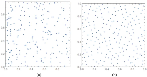
Quasi Monte Carlo technique differs from Monte Carlo in the way that the input samples are generated.Monte Carlo uses pseudo-random samples whereas quasi Monte-Carlo uses a low discrepancy sequence like Sobol’s sequence. This difference is illustrated in Fig. 2.1.
The main advantage of using a low discrepancy sequence is that a faster rate of convergence is obtained. Quasi Monte Carlo has a rate of convergence which is O(1/N).
2.3 Latin Hypercube Sampling
Latin Hypercube Sampling, like Quasi Monte Carlo attempts to generate points that are evenly distributed over the entire random space of the input parameters.
This is achieved by partitioning the input distribution into multiple intervals of equal probability and selecting one sample from each interval. Doing so prevents clustering of points that could happen when pseudo-random sequences are used. LHS sampling is illustrated in Fig. 2.2. Like Quasi Monte Carlo, LHS sampling has a better convergence than Monte Carlo which is O(1/N).
(a) (b)
Fig. 2.1: Difference between a low discrepancy sequence and pseudo-random sequence. (a) Pseudo random sequence (b) Sobol’s sequence
2.4 Generalized Polynomial Chaos (gPC) Theory
The concept of orthogonal polynomials has existed for a long time [44]. Polynomial Chaos Theory was first introduced only for Hermite orthogonal polynomials and was called ‘Hermite-Chaos’. However, due to the need to solving differential equations in the presence of uncertainty for a large number of engineering disciplines, the polynomial chaos technique was extended to include other orthogonal polynomials and was renamed as the generalized Polynomial Chaos (gPC) theory.
Consider a network where the input uncertainty is represented by one random variable, λ occupying the random space Ω. Provided the variables have finite second order moments, the uncertainty in the network response X(t,λ) is modeled using gPC theory and is represented as an expansion of orthogonal polynomials and their coefficients.
0)
(
)
(
)
,
(
k k kt
c
t
X
(2.3)where ck(t) represents the coefficient as a function of time and
k(
)
is a unidimensionalorthogonal polynomial basis with respect to the probability distribution function (PDF) of the input random variable. The expansion in 2.3 is truncated to
m k k kt
c
t
X
0)
(
)
(
)
,
(
(2.4)where m represents the order of expansion of the polynomial and there are m+ 1 terms in the expansion. The polynomials
k(
)
are orthogonal with respect to the PDF of the random input parameter λ. ij i j i j i
d
2 ) ( ) ( ) ( ) ( ) (
(2.5)where <,> represents the inner product operation, ρ represents the PDF of λ,
i2is a constant andij
is the Kronecker delta function. The constant term
i2 is used as a normalizing factor to generate orthonormal polynomials. It is important to note that polynomials need to be chosen based on the Wiener-Askey scheme [44], which states that there is a one-one correspondence between the distribution of the polynomials and the kind of orthogonal polynomial used in the expansion. This guarantees the fastest rate of convergence for the PC expansion which is exponential. The corresponding class of orthogonal polynomials with respect to standard distributions can be found in Table 2.12.4.1 One-dimensional orthonormal polynomials
Consider the standard normal distribution N(0,1) where the PDF ρ(λ) is represented as
2 2 2 1 ) (
e (2.6)According to Table 2.1, the Hermite polynomials are the appropriate orthogonal polynomials to the normal distribution. These polynomials can either be generated in an analytic manner [44]
2 2 2 2 ) 1 ( ) ( e d d e H k k k k (2.7)
or using a three-term recurrence relation
Table 2.1: Polynomials and their corresponding distributions
Distribution of λ Orthogonal Polynomials Support
Gaussian Hermite (-∞,∞)
Uniform Legendre [-1,1]
Beta Jacobi [-1,1]
)
(
)
(
)
(
1 1
k
k kH
kH
H
(2.8)From 2.7, it can be observed that
H
0
1
andH1. The normalizing factor for Hermite polynomials can be obtained as!
)
(
),
(
H
k
H
k k
(2.9)Similarly, considering the standard uniform distribution U(-1,1), the PDF ρ(λ) is represented as
otherwise 0 1 1 2 1 ) ( (2.10)
According to Table 2.1, the Legendre polynomials are the appropriate orthogonal polynomials to the uniform distribution. These polynomials too can either be generated in an analytic manner [44] k k k k k d d k P ( 1) ! 2 1 ) (
2
(2.11)or using the three-term recurrence relation
)
(
1
)
(
1
1
2
)
(
1 1
k k kP
k
k
P
k
k
P
(2.12)From 2.11, it can be observed that
P
0
1
andP1 . The normalizing factor for Hermite polynomials can be obtained as1
2
1
)
(
),
(
k
P
P
k
k
(2.13)For ease of understanding, the first six univariate orthonormal Hermite and Legendre polynomials are listed in Table 2.2
2.4.2 Multidimensional orthonormal polynomials
Most practical applications deal with uncertainty quantification in the presence of multiple random variables. In this subsection, generation of multidimensional orthonormal polynomials using univariate orthonormal polynomials is discussed. Consider a general network where the input uncertainty is represented by n mutually uncorrelated random variables
] ,.... ,
[
1
2
n λ . The PC approach approximates the uncertainty in the response X(t, ) as
1 0)
(
)
(
)
,
(
P k k kt
c
t
λ
λ
X
(2.14)The expansion is truncated to P+1 terms which is given by
!
!
)!
(
1
n
m
n
m
P
(2.15)The multivariate polynomials
k(
λ
)
are now orthonormal to the joint probability distributionfunction (PDF) of the input random variables. Since the variables are independent, their joint PDF can be expressed as the product of their individual PDF’s.
Table 2.2: Univariate orthonormal Hermite and Legendre polynomials
Index k Orthonormal Hermite polynomial
(
)
k
H
Orthonormal Legendre polynomialP
k(
)
0 1 1 1 λ
3
2 (
21) 2 ) 2 1 2 3 ( 5 2 3 (
33
) 6 ) 2 3 2 5 ( 7 3 4 (
46
23) 2 6 ) 8 3 8 30 8 35 ( 3 4 2 5 (
5 10
315
) 2 30 ) 8 15 8 70 8 63 ( 11 5 3ij i j i j i
d
2 ) ( ) ( ) ( ) ( ) (
λ λ λ λ λ λ (2.16)The multivariate polynomial basis can be obtained as the product of the univariate polynomial basis across each dimension
n i n i i i k k i k m 1 1 ) ( ) (
λ (2.17)From 2.16 and 2.17, it is evident that the inner product in 2.16 equals
i2only when both multidimensional polynomials are the same and 0 otherwise.For illustration purposes, the generation of two-dimensional basis is shown below.
It is noted that the total degree across both dimensions remains constant in each row and is incremented row by row [44].
2.4.3 Derivation of statistics
The major benefit of using the gPC approach to model the uncertainty in any system is that all the statistical information of the response is contained in the PC coefficients. The mean and variance of the output can be obtained as a function of the coefficients by integrating over the random space Ωn. To obtain the PDF and other higher order statistical moments, the PC
) ( ) ( ) ( ) ( ) ( ) ( ) ( ) ( ) ( ) ( ) ( ) ( ) ( ) ( ) ( ) ( ) ( ) ( ) ( ) ( ) ( ) ( ) ( ) ( ) ( ) ( ) ( ) ( ) ( ) ( 2 4 1 0 2 3 1 1 2 2 1 2 2 1 1 3 2 0 1 4 2 3 1 0 2 2 1 1 2 1 1 2 2 0 1 3 2 2 1 0 2 1 1 1 2 0 1 2 2 1 1 0 2 0 1 1 2 0 1 0
metamodel is probed at a large number of Monte Carlo samples. In this subsection, derivation of the statistical information is explained. The temporal dependence of the terms in the expansion is removed for convenience.
The expected value or the mean of the response X(λ) is represented as
P k k k d c d X X E n n 0 0( ) ( ) ( ) ) ( ) ( )) ( ( λ λ λ λ λ λ λ λ (2.18)It is noted that the first
0(
λ
)
is always equal to 1 for all orthonormal polynomials.0 0 0( ) ( ) )) ( (X c c E P k k k
λ λ λ
(2.19)Therefore, the mean or expected value of the response is just the first coefficient in the expansion.
The variance of the response X(λ) is represented as
P k P k k k j k j k P k k k c c c c d c c d c c X E X E X Var n 0 1 2 2 0 2 2 0 P 0 k P 0 j 2 0 0 0 2 ) ( ) ( ) ( ) ( ) ) ( ) ( ( ))) ( ( ) ( ( )) ( ( n λ λ λ λ λ λ λ λ λ λ λ
(2.20)The variance is the sum of squares of all coefficients except the first. Any general Mth higher order moment can be expressed as
λ λ λ λ λ λ d X E X X E X E M M m n ) ( ))) ( ( ) ( ( ))) ( ( ) ( (
(2.21)Any higher order moment can be computed by generating a large number of Monte Carlo samples based on the input distribution. Since the PC metamodel is already known, it is not required to simulate the network at all the sample points. The PC metamodel is probed at all the samples and the values of the response X(λ)is substituted in 2.21 to easily obtain any higher order statistical moment.
2.5 Intrusive and non-intrusive methods
In this section, approaches to determine the unknown coefficients of 2.3 are discussed. These unknown coefficients are obtained either using intrusive or non-intrusive techniques.
2.5.1 Intrusive methods
Intrusive methods are one of the ways in which the unknown coefficients of the PC metamodel are computed. Intrusive methods like Stochastic Galerkin (SG) are highly accurate and require the construction of an augmented and coupled deterministic network [7]-[22]. The unknown PC coefficients are then determined by a single run of this augmented deterministic network. The main disadvantage of the SG approach is that this augmented and coupled deterministic network is cumbersome to develop. Since the augmentation is P+1 times, the CPU time and memory costs scale in a near exponential manner with respect to the number of random dimensions. Since a separate solver is required for the SG approach, it cannot make use of existing deterministic SPICE solvers for the given network. Furthermore, for non-linear circuits, the SG approach uses lumped dependent sources which further augment the network [15]. Due to these reasons, the SG approach is favorable for simple circuits with small number of random parameters.
The intrusive formulation of the Stochastic Testing (ST) approach was developed to address the inefficiencies of the SG approach [37]. The ST approach solves the coupled system of equations of the augmented circuit, but in a decoupled manner at each time point. Like non-intrusive methods, the coupled equations are solved at P+1 sampling points which are obtained using a node selection algorithm [37]. Unlike the SG approach, the ST approach can be parallelized since the equations are solved in a decoupled manner. The main disadvantage of the ST approach is that the node selection algorithm does not guarantee the best selection of simulation nodes. For more details of the ST approach, readers are encouraged to read [34], [37].
2.5.2 Non-intrusive methods
Non-intrusive approaches to determine the unknown gPC coefficients are attractive because they do not require the development of new deterministic network solvers. Existing SPICE solvers can be used to simulate the network at the determined simulation points. Also, since the simulations are independent of each other, they can be parallelized leading to greater speedup when compared to intrusive approaches. Popular intrusive approaches are discussed in this section.
2.5.2.1 Pseudo-spectral collocation
In the pseudo-spectral collocation approach, the output is expanded in a series or orthogonal polynomials using the gPC expansion and numerical integration techniques are used to determine the PC coefficients [26]. Numerical integration with Gaussian quadrature techniques approximate the integral of a function F(λ)as a weighted sum of function values computed at predetermined sample points
Q i i i w F d F n 1 ) ( ) ( ) ( ) (λ
λ λ λ λ (2.22)where Q is the total number of simulation points given by
Q
(
m
1
)
n, λi [
1i,
i2,...
in],)
(
iF
λ
is the value of the function F evaluated at λiandw
(
λ
i)
represents the weight corresponding to the node λi. For a one-dimensional problem, are the roots of the one-i dimensional polynomial corresponding to the input distribution according to the Askey scheme. For an n-dimensional problem, Q is given by the tensor product of the one-dimensional polynomial roots taken across all n dimensions.In order to determine the unknown gPC coefficients ck, using Gaussian quadrature
integration rules, the projection theorem is used, which performs an orthogonal projection on to the polynomial basis as
Q i i i k i k k k k k k X t w d t X X c n 1 2 ( , ) ( ) ( ) ) ( ) ( ) , ( , , λ λ λ λ λ λ λ
(2.23)The nodes are obtained as the roots of the polynomial. Another way to obtain nodes and their corresponding weights
w
(
λ
i)
is by solving an eigenvalue problem which is known as the Golub-Welsh algorithm [61].The main advantage of the pseudo-spectral collocation approach is that for moderate number of random dimensions, the number of simulations required will be far lesser than that required for Monte-Carlo. For higher dimensional problems, since the number of required simulations scales in an exponential manner with respect to the number of random dimensions, the pseudo-spectral collocation approach, when used to find the PC coefficients fails to provide any benefits. In such scenarios, it is beneficial to use Monte-Carlo to compute the problem statistics.
2.5.2.2 Conventional Linear Regression approach
The conventional linear regression approach is another non-intrusive way of finding the gPC coefficients. It takes advantage of the linear least squares technique to find the best fit for the PC coefficients [48]. This approach begins by approximating the uncertainty in the network response as shown in 2.14. The expansion of (2.14) is oversampled at M = 2(P+1) nodes located within the random space Ω in order to achieve the best possible fit of the PC coefficients over the entire n-dimensional random space Ω [48]. This results in the formulation of an overdetermined system of linear algebraic equations [38]
E
ε
X
A
~
(2.24) where M M P M P M P
1 ) ( ) 1 ( 0 ) ( ) ( 0 ) 1 ( ) 1 ( 0 ; ) ( ) ( ; ~ ; ) ( ) ( ) ( ) ( ε λ X λ X E X X X I λ I λ I λ I λ A (2.25)2.24 can now be solved in a least square sense to obtain the PC coefficients as E
A A A
X~ ( T )1 T (2.26)
A detailed description of the linear regression methodology is provided in Chapter 3. The main benefit of the linear regression methodology compared to pseudo-spectral collocation is that the number of simulations required is M = 2(P+1) which means that it scales in a polynomial fashion with respect to the number of random dimensions as opposed to the exponential scaling. This provides significant savings in CPU costs and makes it an attractive approach for large dimensional problems. The main drawback of using the conventional linear regression approach
is that it uses the Fedorov algorithm based on the D-optimality criteria to select the M nodes which involves a (P+1)X(P+1) size matrix inversion at each stage in the node selection process. This leads to exorbitant CPU costs for finding the nodes. Novel methodologies to mitigate these costs are discussed in Chapter 3.
2.5.2.3 Non-intrusive formulation of Stochastic Testing
The non-intrusive formulation of the Stochastic Testing approach [34] requires less number of nodes when compared to the conventional linear regression approach. The ST approach samples 2.14 at only M P( 1) points in the random space. The resultant system of equations can be expressed as
) ( ) ( ) ( ) ( ) ( ) ( ) ( ) 1 ( 0 ) ( ) ( 0 ) 1 ( ) 1 ( 0 M P M P M P λ X λ X X X I λ I λ I λ I λ (2.27)
The methodology to select the M nodes is described below.
The major challenge in the ST approach is determination of testing nodes since poor selection of nodes results in ill-conditioned matrices which in turns makes the solution inaccurate or impossible to obtain. In order to address this issue, the ST approach of [34] starts with
n
m
1
)
(
nodes obtained by taking the tensor product of the (m+1) unidimensional roots of the polynomial orthogonal to the joint distribution of input random variables. In order to have accurate results, the algorithm states that all the nodes need to be arranged in the descending order of their weights and the first node λ(1)is taken to be the one with the highest weight. The vector V is defined as) ( ) ( ) 1 ( ) 1 ( λ H λ H V (2.28)
where H(λ(k)){
0(λ(k)),
1(λ(k)).,...,
P(λ(k))}T. Assume that r-1 candidate nodes have already been selected. The vector space that spans these r-1 nodes can be represented as)}
(
),...,
(
),
(
span{
(1) (2) ( 1)
λ
rH
λ
H
λ
H
V
(2.29)Now any node λ(r)is considered to be a candidate node if
H
(
λ
(r))
has a large enough orthogonal component to V. This is determined as follows ) ( )) ( ( ) ( ) ( ) ( ) ( r r T r v v λ H λ H V V λ H (2.30)
where is a predefined constant. If the condition in 2.30 is satisfied,
H
(
λ
(r))
is added to the vector span V.The node selection algorithm used in the ST approach is faster than the linear regression approach as there are no matrix inversions involved. It also requires the least number of network simulations, only P+1 as compared to 2(P+1) required in the linear regression approach. The main drawback here is that the ST algorithm selects the first P+1 nodes with a large enough orthogonal component to V. This does not always guarantee optimal selection of the testing nodes.
2.6 Sparse Polynomial Chaos Techniques
It is common knowledge that the CPU cost to evaluate the unknown gPC coefficients scales in a polynomial fashion with respect to the number of random dimensions. This is the
major bottleneck for most PC approach. To mitigate this, the PC expansion needs to be sparsified. In this subsection, some sparse PC techniques are discussed.
2.6.1 Sensitivity Indices using ANOVA-HDMR
One way to sparsify the PC expansion is to get an understanding of how much of an impact each random input parameter has on the network output and retain only those parameters which have a significant impact on the response. For this purpose, the network response is split into a sum of functions of increasing dimensions known as High Dimensional Model Representation (HDMR). This performs the separation of the effects of the input parameters which are transmitted in the decomposition of the variance [54].
) λ ... λ , ( ... ) λ , λ , ( ) λ , ( ) ( ) , ( ... 12 , 1 1 0 n i n n j i j i ij n i i i t x t x t x t x t x
λ (2.31)where x0 is the nominal value of x(t, ), xi(t,λi) represents the contribution of λi to x(t, ) acting
alone, xij(t,λi, λj) represents the pairwise contribution of λi and λj to x(t, ) etc. The variance of the
response is expressed as
n j i ij N i i n j i j i i N i i i n i n n j i j i i n i i i x n n n n t x d t x d t x t x t x d x t x , 1 2 1 2 , 1 2 1 2 ... 12 , 1 1 2 0 2 .... ... ) λ , λ , ( ) λ , ( )) λ ... λ , ( ... ) λ , λ , ( ) λ , ( ( ) ) , ( ( λ λ λ λ (2.32)Since the impact of each random dimension is studied on the variance of the response, this methodology is called Analysis Of Variance (ANOVA). Sensitivity indices quantify the contribution of each parameter on the output variance. They are expressed as
n i i S s x i i i i i i s s 2 1 1 ... 2 ... ... 2 1 2 1
(2.33)The total sensitivity index of a parameter
i represents the total effect of
i on the output variance. It is represented as n ijk n i j j ij i TiS
S
S
S
1.. .. , 1....
(2.34)The PC expansion can be used to compute the sensitivity indices of each input dimension by rearranging the terms in the expansion to resemble those in the HDMR expansion. Since all the statistical information in the PC expansion is contained in the coefficients, the sensitivity indices can easily be expressed in terms of the PC coefficients.
The main issue with using this method is that, in order to compute the sensitivity indices, all the PC coefficients need to be computed. Although, the dimensionality of the network can be reduced by only considering dimensions with significant values of the sensitivity index, the CPU costs scale in a polynomial fashion with respect to number of dimensions. In order to mitigate this cost, a novel reduced dimensional PC approach is proposed in Chapter 4.
2.6.2 Hierarchical Sparse PC Approach
The hierarchical sparse PC approach is another technique to develop a sparse PC expansion and mitigate the poor scalability of the gPC approach. This method also uses the
HDMR formulation but in an iterative manner by including only the component functions pertinent to the most important random parameters [40], [41].
Consider the HDMR expansion in 2.31. |u| is defined as the cardinality of a component function. For example, |u| = 1 for
x
i(
t
,
λ
i)
, |u|=2 for xij(t,λi,λj)and so on. The iterative algorithm first computes the weights associated with a component function as1 u ) , ( ( 0 x t x E u λ γ (2.35)
If u exceeds a prescribed tolerance, then the random variable corresponding to the component
function is considered to be significant. Next, the second order component functions corresponding to only the significant random dimensions are considered as candidates for constructing the second level HDMR. The associated weights are recomputed as
2 u ) , ( ( ) , ( ( 1
u v v v u u u t x E t x E γ (2.36)This process continues in an iterative manner until the HDMR converges. At the third level, only the third level interactions of the important second order component functions are considered.
The hierarchical sparse PC approach uses very few terms in the PC expansion owing to its selection/eliminations. This reduces the computational effort to a large extent. The main drawback of this approach is that the error of the PC expansions representing the lower order interactions gets propagated to the higher levels. More details are given in Section 4.
2.6.3 Anisotropic Sparse PC Approach
The Anisotropic Sparse PC (APC) approach is based on the insight that each random dimension does not have equal impact on the network responses. As a result, the maximum degree of expansion along each dimension can be tuned to different values based on the magnitude of the impact each dimension has on the network response. This is in contrast to existing isotropic sparse PC approaches where the expansion requires the maximum degree of expansion along all dimensions to be equal and set to a common value. Due to the intelligent tuning of the maximum degrees of expansion along each dimension, an anisotropic PC expansion will be substantially sparser than a full-blown PC expansion and hence the associated coefficients can be evaluated far more efficiently.
The APC approach in [73] starts with the HDMR expansion in 2.31. The impact of each random dimension on the response x(t,λ) acting along is quantified using the concept of cut-HDMR whereby
)
(
)
,
(
)
,
(
)
,
(
)
(
0 λ \ ) 0 ( 0 ) 0 (x
t
t
x
λ
t
x
t
x
t
x
i i i
λλ
λ
(2.37)The notation λ(0) \λi represents the vector where all component of except λ
i is set to 0.Based
on (2.37), these impact terms can be expressed using 1D PC expansions as
i i m 1 j i j j i t x t x t x( , ) λ 0( ) ( )( ) (λ ) \ ) 0 (
λ λ (2.38)where xi(j)(t) represents the jth coefficient and ϕj is the corresponding 1D basis chosen from the
Weiner-Askey scheme.
An iterative approach is used to determine the value of mi. Its value is initially set to one and the
coefficients are obtained, then the value of mi is iteratively increased in steps of one and in each
iteration the new coefficients of (2.38) are evaluated using the same pseudo-spectral method. After the computation of coefficients, the normalized enrichment in the variance predicted using the 1D expansion arising from the increment in the degree of expansion is evaluated as
1 1 2 ) , ( 1 2 ) 1 , ( 1 1 2 ) , ( ) ( r j r j i r j r j i r j r j i i x x x t S (2.39)where r refers to the current iteration. Once the enrichment falls below a prescribed tolerance , the iterations are halted.
Once the degree of expansion along all the random dimensions is known using the above methodology, an anisotropic PC expansion of the network response x(t,λ)can be formulated as
Q 0 k k k t t, ) ( ) ( ) ( λ X λ X (2.40)where the multidimensional basis k( ) is a product of 1D basis as
N i i k k i 1 ) ( ) ( λ (2.41)with the constraint that
N N
m
k
m
k
m
k
1
1;
2
2;
...;
(2.42) 2.6.4 Hyperbolic PC ExpansionThe Hyperbolic PC Expansion (HPCE) is another sparse PC technique which uses an alternative hyperbolic truncation scheme instead of the conventional linear truncation scheme.
This choice of the hyperbolic truncation scheme is based on the sparsity of effects principle which claims that the dominant effect on the response uncertainty comes from the impact of each
random variable acting alone and their low-degree interactions. Guided by this principle, the hyperbolic truncation scheme automatically prunes the statistically insignificant high-degree multidimensional bases from a general PC expansion.This hyperbolic truncation scheme results in a substantially sparse PC formulation which is numerically more efficient to construct than the conventional alternatives [59].
Traditionally, for uncorrelated random variables, any arbitrary kth multidimensional basis can be expressed as a product of one dimensional bases as
k k n i i n i i k k
i
1 1 ; ) ( ) (
λ (2.43)where K = [k1, k2, …, kn] is the vector of the 1D PC degrees.Such a truncation scheme where all relevant PC bases are enclosed between the hyperplane ||K||1 = m and the positive axes representing the random dimensions is referred to as the classical linear truncation scheme. In the
λ1 λ2 λ1 λ2 λ1 λ2 1 ; || || 1 1m u u K || || ; 1 2 1 2m u u u K || K||1m
Fig. 2.4: Illustrative example demonstarting the sparsity due to the proposed hyperbolic truncation crietrion over the classical linear truncation crietrion using a 2D example (n = 2, m = 5). The decrease in sparsity with the increase in the hyperbolic factor (u) is shown. At u = 1, the proposed HPCE expansion coincides with the full-blown PC expansion.
hyperbolic truncation scheme, by pruning the high-degree multidimensional bases from the expansion of (2.14), a sparser PC formulation can be achieved. This hyperbolic truncation scheme is described using the fractional u-th norm of K as
;
0
1
/ 1 1
u
m
k
u N i u i uK
(2.44)where u is the hyperbolic factor. The hyperbolic truncation scheme of 2.44 ensures that only those multidimensional bases of 2.14 lying under or on the hyperbola ||K||u = m, as opposed to a
hyper-plane ||K||1 = m, are retained in the expansion. In other words, due to the non-zero radius of curvature of the hyperbola ||K||u = m, the higher-degree multidimensional bases of 2.14 will be
pruned from the expansion. This selective pruning of the PC bases will ensure the best accuracy of the expansion while leading to a sparser formulation than 2.14.
It is noted from Fig. 2.4 that the sparsity achieved by the HPCE depends on the radius of curvature of the truncating hyperbola which in turn depends on the hyperbolic factor u. Therefore, by tuning u it is possible to adapt the HPCE to exhibit the best sparsity-accuracy tradeoff. The main disadvantage of using the HPCE method is that it lacks control over the number of bases pruned because of the hyperbolic factor u takes specific values. So, for large problems, even the penultimate value of u prunes a large number of bases which causes the HPCE method to become inaccurate.
CHAPTER3:APPROACHESTOACCELERATETHECLASSICALFEDOROVSEARCH ALGORITHM
From the previous chapter, it is evident that among the non-intrusive techniques to evaluate the PC coefficients, the linear regression approach is preferred as it uses only a sparse subset of nodes out of the entire tensor product set of nodes without compromising on the accuracy of the results. However, for large dimensional problems, the traditional search algorithm takes a large amount of time for selecting the DoE nodes. In this dissertation, firstly, the methodology used by the traditional linear regression to select the DoE using the D-optimality criterion and the Fedorov search algorithm is explained. Next, two novel numerical strategies are proposed to expedite the search for the substitute DoE for problems involving high-dimensional random spaces. As the first strategy, instead of substituting all DoE, the proposed algorithm identifies a small fraction of the worst DoE present in the initial selection and replaces only these DoE. As the second strategy, a recursive method to efficiently compute the inverse of the information matrix required for every exchange of DoE is developed. Further, a complexity analysis of the search algorithm in [36] is presented. The accuracy and efficiency of the proposed approaches is illustrated by comparing the results with other PC approaches for microwave/RF networks using multiple numerical examples.
3.1 PC expansion using Linear Regression
Consider a general microwave/RF network where the uncertainty in the physical dimension, circuit elements, and electrical properties of the network is represented by n mutually uncorrelated real valued random variables = [λ1, λ2,…, λn]Tlocated within the multidimensional
random space Ω. In order to extract all the statistical information of this network, the variability in the network response is approximated using a PC expansion as
ε
λ
X
λ
X
P 0 k k kt
t
,
)
(
)
(
)
(
(3.1)where is the vector of random truncation errors of the PC expansion. The Linear Regression approach begins by oversampling the expansion of (3.1) at M = 2(P+1) nodes located within the random space Ω. The expression of (3.1) is oversampled in order to achieve the best possible fit of the PC coefficients over the entire n-dimensional random space Ω [43]. This results in the formulation of an overdetermined system of linear algebraic equations [43]
E
ε
X
A
~
(3.2) where M M P M P M P
1 ) ( ) 1 ( 0 ) ( ) ( 0 ) 1 ( ) 1 ( 0 ; ) ( ) ( ; ~ ; ) ( ) ( ) ( ) ( ε λ X λ X E X X X I λ I λ I λ I λ A (3.3)and I represents the identity matrix. The vectors εj of (3.3) are the individual truncation errors at
each node. The vector E consists of the network responses obtained by probing the original stochastic network of (3.1) at the M multidimensional nodes (or DoE) (j) = [λ1(j), λ2(j),…, λn(j)];
M j
1 . Equation (3.3) can now be solved in a least-square sense to evaluate the PC coefficients of the network response. Once the PC coefficients are obtained from (3.3), all statistical moments of the network responses can be obtained from the PC expansion of (3.1).
3.2 Advantages over intrusive approaches
A key benefit of the conventional linear regression approach is that sophisticated deterministic solvers such as SPICE can be directly used to populate the matrix E in (3.3) without any intrusive coding as required in the SG approach and the stochastic testing approach [7]-[22], [37]. More importantly, the M SPICE simulations of (3.3) can be easily parallelized unlike the SG approach.
3.3 Proposed D-Optimal Linear Regression Approach
In order to identify the M nodes satisfying the D-optimal criteria for the regression problem of (3.3), in this dissertation, we propose to utilize the Fedorov search algorithm which has been commonly used in the field of estimation theory and experimental designs [46],[48]. While there are various other exchange algorithms besides the Fedorov algorithm, the work of [46] demonstrates that the Fedorov algorithm reaches successful completion far more frequently than its counterparts. The following subsections explain the rationale behind the choice of the D-optimal criterion, the Fedorov search algorithm to identify the D-D-optimal nodes and the computational cost associated with the search.
3.3.1 D-optimal Criterion
The importance of the D-optimal criterion to the accuracy of the evaluated PC coefficients of (3.3) is revealed using the following lemma.
Lemma 1μ Assuming that the truncation error j 1 jM at all M DoE of (3.3) are independent
to achieve the maximum accuracy of the PC coefficients the DoE must be chosen such that the determinant of the information matrix AtA of (3.2) is maximized.
Proof: Based on the PC expansion of the network responses of (3.1), it is understood that the
presence of the random truncation error ε makes the PC coefficients themselves random variables. The variance of the evaluated PC of (3.3) can be computed as
t t t t t t t Var Var Var ) ) )(( ( ) ( ) ) (( ) ~ ( 1 1 1 A A A E A A A E A A A X (3.4)
Knowing that the truncation error for each DoE (i.e., εj) is independent and has a constant
variance σ2, Var(E) = σ2I where I is the identity matrix. Replacing this in (3.4) the variance of the PC coefficients of (3.4) can be compactly expressed as
2 1 ) ( ) ~ (X AtA
Var (3.5)From (3.5) we understand that to ensure the maximum accuracy of the PC coefficients we have to reduce the uncertainty in the solution X~ (i.e., the variance of X~ ). Since the variance of X~
is inversely proportional to the determinant of the information matrix AtA, a simple way to minimize the variance of X~ is to maximize the determinant. This criterion is referred to as the D-optimal criterion [46], [47]. It is noted that other optimal criterions besides the D-optimal criterion also exists although the D-optimal criterion has been deemed the most effective and popular till now [46]. In the next subsection, we develop a search algorithm that can efficiently identify the D-optimal nodes from multidimensional random spaces.
3.3.2 Greedy Search Algorithm to Identify DoE
In this subsection, the development of a greedy search algorithm to identify the D-optimal DoE from multidimensional random spaces is described. This greedy search algorithm is


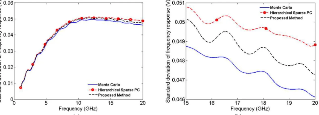
![Fig. 4.3: Statistical analysis of Example 1 using proposed approach, the work of [41] and [59], all compared against Monte Carlo approach (25,000 samples)](https://thumb-eu.123doks.com/thumbv2/5dokorg/4331247.98100/77.918.121.779.604.853/statistical-analysis-example-proposed-approach-compared-approach-samples.webp)