THESIS
ANALYSIS OF PRODUCED WATER FROM THREE HYDRALICALLY FRACTURED WELLS WITH
DIFFERENT LEVELS OF RECYCLED WATER
Submitted by
Brian E. McCormick
Department of Civil and Environmental Engineering
In partial fulfillment of the requirements
For the Degree of Master of Science
Colorado State University
Fort Collins, Colorado
Spring 2016
Maste ’s Co ittee:
Advisor: Kenneth Carlson
Sybil Sharvelle John Stednick
Copyright by Brian E. McCormick 2016
ABSTRACT
ANALYSIS OF PRODUCED WATER FROM THREE HYDRALICALLY FRACTURED WELLS WITH
DIFFERENT LEVELS OF RECYCLED WATER
With the growing use of hydraulic fracturing, injecting large amounts of water into oil
and natural gas reservoirs to increase the quantity of oil and natural gas extracted, large
amounts of water with low water quality are being created. This water has to be disposed of
and many disposal methods have environmental concerns. One method of disposal is treating
the water to remove the contaminants that have environmental concerns. Treatment of
produced water for reuse, which will be identified as recycled water, as a fracturing fluid is
becoming an increasingly important aspect of water management surrounding the
unconventional oil and gas industry since the treatment does not have to be as robust as it
would for disposal into surface water. Understanding variation in water quality due to
fracturing fluid and produced water age are fundamental to choosing a data driven, water
management approach. For these reasons, Noble Energy partnered with CSU to analyze the
water quality differences between four wells with different levels of recycled water usage in a
previous study. In that study, the findings showed a higher organic content of the produced
water in the early period due to the presence of emulsified oil. The higher organic content of
that produced water was the reason for using recycled water at more wells to determine if the
percent fresh water, another well was one part recycled water and five parts fresh water, and
the last well was one part recycled waters and seven parts fresh water.
Based on the data, the inorganic constituents vary more than the organic material.
Inorganic variance being greater than organic makes sense due to the fact that the organic atte o es ai l f o the f a tu i g fluid’s gel or slickwater component (Sick 2014), despite the organic variance seen in the previous study (White 2014). The inorganic matter
mainly comes from the recycled water as seen from the ANOVA testing indicating significant
difference between the wells, which is not treated to fresh water levels, and the data from the
three wells shows a significantly higher value for the wells fractured with recycled water. A
good illustration of the difference in the produced water quality that can be tied to the
fracturing water quality is the TDS that was between four and six times higher in the fracturing fluid’s ase fluid due to the use of recycled water. Of the inorganic constituents measured, aluminum, silicon, zinc, ammonium and sulfate were the only ones that did not show a
statistically significant difference between the fresh water well and the recycled wells as
indicated by a p value of 0.05 from an ANOVA test. None of the organic constituents showed
significant statistical difference between the recycled wells and fresh water well, but they did
vary over time indicating that the reactions and interactions with the geological formation
affected the wells at a different rate.
The wells did show a statistical difference both between the wells and over time,
however, not in the way that was hypothesized as the organic material did not vary based on
the wells. Total organic carbon (TOC), dissolved organic carbon (DOC), oil range organics (ORO),
0.349, 0.768 and 0.707, respectively. The organics showed more significant difference over
time with TOC, GRO, and ORO with p-values of 0.005, 0.012, and 0.029, respectively. However,
the inorganic data did show significant difference between wells as well as over time. The
inorganic constituents boron, barium, bromide, calcium, iron, potassium, magnesium, chlorine,
strontium, sodium, and bicarbonate all had p-values of less than 0.01 except for chlorine which
was 0.014. Potassium was the only constituent in that list that was not significantly different
over time, but silicon and ammonium, which did not differ by well, did show significant
difference over time. All of the inorganic constituents were very significantly different over
time with no p-value over 0.01. The impact of this on the water management strategies shows
that the understanding of the produced water quality and the factors that impact that is still
largely unknown. More sampling and testing for well variability based on the ratio of recycled
water in the fracturing fluid will allow more data and a better data driven management
ACKNOWLEDGEMENTS
Writing acknowledgements for a thesis is a bit surreal for me. Even now with the end in
sight, I look back and wander how I got here. However, it does not take me long to fully
appreciate the fact that I would not be here without the help, guidance and support of so
many.
To Dr. Ken Carlson, my advisor, thank you for the patience to put up with my growing
pains. I have learned more from my time here than just water chemistry. I can promise that
my career growth is only comparable to my growth as an individual and I appreciate the part
you played in that.
To my other committee members, Drs. Sybil Sharvelle and John Stednick, thank you very
much for taking time out of your schedule to sit on my committee. I can only imagine that
there are other things you would much rather spend your time on. I hope that I have offered
even a nugget of value to you.
I would also like to thank Ashwin Dhanasekar, Drew Caschette, Wanze Li, Marth Nuñez,
Shane White, Seongyun Kim, and Bing Bai for all their help gathering the samples, testing them
and their support in the writing of this thesis. I would especially like to thank Seongyun who
pointed me in the direction of this topic and was instrumental in teaching me how to write a
thesis.
I would also like to thank my family for being there for me and being some of the
TABLE OF CONTENTS
ABSTRACT ...ii
ACKNOWLEDGEMENTS ... v
LIST OF TABLES ... viii
LIST OF FIGURES ... ix
1. Introduction ... 1
2. Literature Review ... 3
2.1 The United States and Oil and Gas ... 3
2.2 Hydraulic Fracturing ... 6
2.2.1 Background ... 6
2.2.2 Effects... 7
2.2.3 Extraction ... 8
2.2.4 Contentious Nature of Hydraulic Fracturing ... 14
2.3 Water Management and Treatment ... 18
2.3.1 Disposal ... 20
2.3.2 Recycling ... 23
2.4 Research Purpose and Objective ... 25
3.1 Introduction and Purpose ... 30
3.2 Fracturing Fluid ... 30
3.3 Sample Collection ... 32
3.4 Methods ... 33
3.4.1 Analysis Performed at CSU... 33
3.4.2 Analysis Performed by eAnalytics ... 35
3.4.3 Data Analysis Techniques ... 36
3.5 Results ... 39
3.5.1 Gravimetric Solids and Turbidity... 39
3.5.2 TOC and DOC ... 48
3.5.3 pH, Alkalinity and Carbohydrates ... 51
3.5.4. LC-MS ... 56
3.5.5. eAnalytics Testing Analysis ... 62
4. Conclusions ... 68
5. Future Work ... 69
LIST OF TABLES
Table 2-1. Typical Fracturing Fluid Components ... 12
Table 2-2. Crow Creek Wells Compared to Chandler State Wells ... 26
Table 3-1. Fracturing Fluid Composition As Found On FracFocus.org ... 31
Table 3-2. Total Dissolved Solids in Fracturing fluids ... 32
Table 3-3. Total Solids for All Three Wells Sampled ... 39
Table 3-4. ANOVA Results for Gravimetric Solids ... 43
Table 3-5. Volatile Solids Data ... 46
Table 3-6. ANOVA Data ... 51
Table 3-6. pH, Alkalinity and Carbohydrates Data ... 52
Table 3-7. ANOVA Data ... 53
Table 3-7. Compounds Found in the Samples Via LC-MS-EIS Negative Characterization ... 59
Table 3-8. Compounds Found in the Samples Via LC-MS-EIS Positive Characterization ... 61
Table 3-9. ANOVA Results for Inorganic metals and Compounds ... 62
LIST OF FIGURES
Figure 2-1. The Shale Plays of the Lower 48 States ... 6
Figure 2-2. Conventional and Horizontal Well Oil and Gas Production ... 8
Figure 2-3. Cross-section of the Wattenberg Field ... 9
Figure 2-4. Water Usage for Extraction and Processing of Energy Fuels. ... 14
Figure 2-5. Map Showing Location Between Crow Creek and Chandler State ... 27
Figure 2-6. Wattenberg Field in the DJ Basin and the Geologic Formation. ... 27
Figure 2-7. TOC Comparison ... 28
Figure 2-8. Tubidity Comparison ... 28
Figure 3-1. Box Plot of Data Points in TSS, TDS and TS ... 40
Figure 3-2. Comparison of the Three Wells for TSS, TDS and TS ... 42
Figure 3-3. Box Plot of Data Points for VSS, VDS and TVS ... 44
Figure 3-4. Temporal Trends of TVS, VDS and VSS ... 45
Figure 3-5. Box Plot of Data Points in Early, Middle and Late Time Periods for Turbidity ... 47
Figure 3- . Tu idit ’s Te po al T e d ... 47
Figure 3-7. Box Plot of Data Points in Early, Middle and Late Time Periods for TOC ... 48
Figure 3-9. TOC and DOC Temporal Trends ... 50
Figure 3-10. pH, Alkalinity and Carbohydrates Temporal Trends... 52
Figure 3-11. Box Plot of Data Points in Early, Middle and Late Time Periods for pH ... 54
Figure 3-12. Box Plot of Data Points in Early, Middle and Late Time Periods for Alkalinity ... 55
Figure 3-14. LC-MS-ESI-Positive Ion Spectrum for All Wells ... 57
Figure 3-15. Mass Spectrum of Flowback from Well F ... 58
Figure 3-16. Box Plot of Data Points in Early, Middle and Late Time Periods for Ammonium .... 64
1. INTRODUCTION
Oil and natural gas production has skyrocketed domestically in the US over the last five
to ten years despite the current downturn. Much of the growth is due to the expanded use of
hydraulic fracturing and horizontal drilling (Ratner and Tiemann 2015), both of which are water
intensive with estimated usage of 2.8 million gallons for hydraulic fracturing and if the it is
extended hydraulic fracturing with 25 stages, the fracturing is separated into stages fractured
individually, uses an estimated 6.5 million gallons (Goodwin 2012). As more wells are fractured
in oil and gas fields, the flowback and produced water (produced water), the wastewater
coming back to the surface of the well, continues to increase and water management strategies
become critically important due to the use of large volumes of water. The Wattenberg Field, in
Weld County, CO is currently at the point where the large amount of water that needs to be
treated has pushed companies to experiment with different treatment, including recycling the
produced water for future fracturing use, and disposal techniques. The treatment currently
centers around the removal of solids from the produced water. Clarifiers and coagulant
addition are the mechanisms currently used for treatment.
Recycling produced water from wells can help minimize the demand on fresh water in
the region. Utilizing recycling would have the benefit of improving a o pa ’s pu li elatio s profile and still maintain favorable economics. The recycling process requires treatment prior
to reuse and can have an effect on the produced water quality. Understanding the differences
This study centered on data gathered from a 36-day sampling timeframe. The samples
gathered were analyzed for many water quality parameters both at CSU and at an outside
EPA-certified laboratory. The goal of the laboratory work was to determine if there was a difference
in the produced water from two wells fractured with one part recycled water with seven parts
fresh water, which will be labeled Well R1, in one well and five parts fresh water in a second
and one fractured only with freshwater in a third, which will be labeled R2.
Chapter 2 of this thesis investigates the literature that might be pertinent to understand
prior to examining the data form the three wells. This section combines many references to
provide an understanding of conventional and unconventional oil and natural gas extraction
techniques, how the industry began fracturing, and why recycling produced water is an
important option for producers continuing to use hydraulic fracturing in the future. The
chapter ends with clearly defined objectives for the research.
Chapter 3 provides background about the well, including the specifics of the fracturing
fluid like TDS. The sampling and analyzing of the sample are described next followed by the
results of the analysis. The results not presented in this section of the thesis that support the
results discussed are also presented in Appendix B and C.
Chapters 5 provides conclusions that can be made from the results presented in
Chapters 3 and 4. Chapter 6 acknowledges certain areas where more research can help provide
more data for better understanding of the recycling process. The references used in the thesis
2. LITERATURE REVIEW
2.1 The United States and Oil and Gas
The global industrial society and its growth have relied and continue to rely heavily upon
oil and natural gas. The extraction of oil and natural gas has gotten more difficult due to the
depletion of the more readily available reservoirs. Technological advances in drilling and
hydraulic fracturing have allowed unconventional methods of oil and gas extraction to become
more attractive financially (Gregory et al. 2011). Unconventional oil and gas plays are locations
where the oil and gas has to be extracted from source rock formations that are highly
compressed with low porosity like shale formations. As more wells are drilled
unconventionally, the technologies that enable unconventional drilling are improving the
practicality of unconventional drilling, both technically and financially. In fact, it is currently one
of the largest and fastest growing sectors of domestic energy production over the last several
years (EIA 2014).
The expansion of the use of unconventional oil and gas extraction, specifically hydraulic
fracturing, has improved the forecast for future domestic production and subsequently has
reduced the projected amount of crude oil and petroleum products that the US is expected to
import. The U.S. EPA Office of Air Quality Planning and Standards agreed with the assumption
that the use of unconventional oil and gas wells will continue to grow (OAQPS 2014).
Specifically, the total share that imports take up in petroleum products is expected to decrease
from 33% in 2013 to 17% in 2040 (EIA 2015). The importance of the petroleum products can be
many products used in the everyday life of Americans and they are heavily involved in
electricity generation. Fossil fuels account for 79.3% of primary energy production in the US
and 81.5% of total consumption. Currently, natural gas makes up 27%, which is still less than
the 39% that is associated with coal usage, of the US energy supply, but is projected to increase
over the coming years and eventually become the most leveraged fuel for electricity production
in the US, surpassing coal (EIA 2014). Furthermore, the pressure on oil and gas and energy
production companies is only expected to increase as global energy demand increases by 37%
by the year 2040 (WEO 2014). Domestically, U.S. energy consumption is expected to grow by
an average of 0.3% per year through 2040, with the industrial sector having the largest gains at
an average of 0.7% per year (EIA 2015).
The projected increase in domestic production is in line with the production increase the
domestic producers have seen over the last several years. From 2008 to 2013, the domestic
production of crude oil increased from a starting position of 5.0 million barrels per day up to 7.4
million barrels per day, a 48% increase. Over the same time period of 2008 to 2013, natural gas
production increased from 20.2 trillion cubic feet per day to 24.3 trillion cubic feet per day, a
17% increase. The i ease i atu al gas p odu tio oi ides ith a i ease i atu al gas’s share of total U.S. energy consumption rising from 23% to 28%. The trend of increasing
production of domestic crude oil and natural gas leads to the prediction of increased
production continuing through year 2040 (EIA 2015). The past increases and future increase
projections are likely due to the decrease in price associated with higher production.
For crude oil, the increase in production annually until 2040 is projected at 0.9%. For
this growth in natural gas production will be increases in the development of shale gas
reserves. The expectation is for domestic production of shale gas, which includes natural gas
from tight geological formations, is to increase from the 11.3 trillion cubic feet produced in
2013 to 19.6 trillion cubic feet in 2040, a 42% increase (EIA 2015). The growth of shale gas
production is heavily influenced by the growth in tight gas but federal offshore and onshore
Alaska productions are also likely to assist in the growth (EIA 2015).
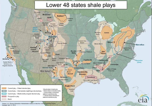
The figure below, Figure 2-1, shows the plays located through the continental United
States (EIA 2015). The plays range from more oil dense areas such as the Bakken, which
produces mainly crude oil out of the North Dakota area, to the Marcellus play that mainly
produces natural gas in the Appalachian area. The variation in the available hydrocarbons at
each play is dependent on the temperatures and pressures of the geological formations (DOW
1977). The differences are important as the areas will have corresponding drilling and
operational needs, as well as distinct regulatory requirements, such as the rule in Pennsylvania
Figure 2-1. The Shale Plays of the Lower 48 States
http://www.eia.gov/oil_gas/rpd/shale_gas.pdf.
2.2 Hydraulic Fracturing
2.2.1 Background
Hydraulic fracturing began in the late 1940s in an attempt, like today, to get more resources
out of each well (EPA 2015). At first, the attempts were conducted in traditional vertical wells
in conventional oil and gas plays. Conventional oil and gas extraction usually utilizes the drilling
of vertical wells into areas that have high permeability, which allows the oil and gas to flow
easily up the well to the ground surface for collection. The high permeability areas generally
consist of sandstone or carbonate solids, and the pressure differential in the well compared to
the surface is enough for the oil and gas to flow freely.
As the oil and gas requirements of industry, as well of the population, have grown,
including horizontal drilling, has allowed unconventional plays to be accessed more easily.
Combined with the horizontal drilling, hydraulic fracturing has allowed the economical
extraction of oil and gas in unconventional fields (EPA 2015). The use of hydraulic fracturing
was not heavily utilized in the industry until the technology and demand allowed the companies
to produce it economically, which did not occur on a large scale until 2003 (MacRae 2012). The
area credited as the first oil and gas play to have economic success with horizontal drilling and
hydraulic fracturing, which led the industry to believe in the possibilities of horizontal drilling
combined with hydraulic fracturing, was the Barnett Shale area of Texas (Gregory et al. 2011). H d auli f a tu i g a d ho izo tal d illi g’s popula it g e ui kl f o that poi t a d so e estimates state that 90% of currently producing wells were originally stimulated with hydraulic
fracturing techniques (MacRae 2012).
2.2.2 Effects
The effect of fracturing has been tremendous for the United States. The reserve
estimates increased by 35% between 2006 and 2009, with the Marcellus Shale production of
natural gas via shale formations being a large reason for the increase (Gregory et al. 2011).
Hydraulic fracturing, has increased US oil production year over year from 2008 to 2009, the first
such increase since 1991. The trend has continued every year since then as well, increasing by
3.2 million barrels per day from January 2008 to May 2014, with 85% of that increase attributed
to shale and tight oil formations in Texas and North Dakota (Ratner and Tiemann 2015). 50% of
onshore crude oil production is expected to come from hydraulic fracturing by 2019 (EIA 2014).
Additionally, energy exports are projected to equal import by 2028 (EIA 2015). Some estimates
The estimated increases are due, in large part, to the assumption that the number of oil and gas
wells will continue to increase in the coming years (OAQPS 2014).
2.2.3 Extraction
This section will explore and expand on the conventional and horizontal drilling with
hydraulic fracturing methods oil and natural gas collection. Figure 2-2 gives a visual
representation of the differences between conventional and unconventional oil and gas
production (Gregory et al. 2011). Both methods are harvesting the hydrocarbons from
geological strata where plant and animal organic matter was deposited and converted over
time into the hydrocarbons (EPA 2004).
Figure 2-2. Conventional and Horizontal Well Oil and Gas Production
In this study, the Niobrara formation is the one being harvested. The Niobrara is a
formation in the Wattenberg Field. The wells in the Wattenberg Field average a depth of
7600-8400 (Smith, Holman et al. 1978). The Wattenberg Field is estimated to have roughly 5.2 trillion
techniques (Dhanasekar 2013). Figure 2-3 shows a cross-section of the Wattenberg field and
the depth of the Niobrara.
Figure 2-3. Cross-section of the Wattenberg Field (http://www.freerepublic.com/focus/f-news/3094221/posts) 2.2.3.1 Conventional
As stated previously, conventional oil and gas wells typically utilize vertical wells that tap
into geological areas that freely release the stored hydrocarbons based on the pressure
differential from the formations to the ground surface. The reservoirs that conventional wells
tap into usually have high permeability with the oil and gas trapped by a geological formation.
This formation prohibits the fluid from leaving the source rock and allows for accessibility for
harvesting the hydrocarbons (Schenk and Pollastro 2002). The permeability is what allows the
extraction of the oil and/or gas to leave the source rock. If the permeability is not high enough,
then the well must be stimulated to increase the permeability and allow for economical
extraction of the hydrocarbons. In terms of water usage, 80 percent of the total water required
for conventional production is consumed in secondary recovery, which uses methods like water
injection to increase pressure in the reservoir, and that number represented 70 percent of
onshore oil production in 2005 (Wu and Chiu 2011). The simplicity of conventional methods is
and natural gas compared to hydraulic fracturing, but it is also what limits the potential
reserves.
2.2.3.2 Unconventional
The source rock for unconventional oil and gas reservoirs has a lower permeability, and
the pressure differential is insufficient to liberate the hydrocarbons for surface flow. Therefore,
the formation must be stimulated. The stimulation in hydraulic fracturing creates fissures and
cracks that increase the permeability of the source rock. Shale is a common source rock that
contains hydrocarbons. Shale is fine-grained and primarily composed of clay minerals and
other particles that are similar in size to silt (Gregory et al. 2011). As shown in Figure 2-2,
fracturing is utilized primarily with horizontal drilling since horizontal wells can replace many
traditional vertical wells, adding additional economic benefits of reducing drilling costs (Arthur
2008). Hydraulic fracturing utilizes high pressures and large amounts of water, therefore, it is
vital that production companies have access to enough water to meet their needs (Gregory et
al., 2011). Approximately two to seven million gallons of water were required for each well
(Ranm, 2011; Stephenson, 2011; Lee, 2011; Nicot, 2012; Suarez, 2012; Goodwin, 2013;
Hickenbottom 2013). The contact length of the well, combined with the hydraulic fracturing is
what allows producers to extract the resource economically (Gregory et al. 2011). Hydraulic
fracturing and horizontal drilling is economically viable despite the high cost associated with
pumping fracturing fluid, which is engineered specifically for each well, and acquisition, which
includes trucking and other costs, and usage of the water and other fracturing fluid additives
fracturing with horizontal drilling uses less drilling overall and thus each well, despite the higher
cost per well, can have a better return on investment (Gregory et al. 2011; Fitzgerald 2013).
2.2.3.3 Fracturing Fluid Characteristics
Hydraulic fracturing fluid is engineered specifically to maximize the extraction potential of
the well. The fluid is composed of many components, as shown in Table 2-1 (DOE 2009).
However, despite the complexity of the mixture for the fracturing fluid, the majority of the
mixture, 99.5%, is water and sand, or some other granular proppant used in place of sand (EPA
2004; FracFocus 2015). The water acts as the carrier fluid that transports the other chemicals
needed to maintain the higher permeability created in the geologic formation, typically shale or
other tight formations, and is used to create the pressure to fracture the strata initially. The
sand or other proppants keep the fractures open so the pressure does not reclose the fractures,
maintaining the permeability of the formation (FracFocus 2015). Once the proppant is in place
to maintain the initial fractures, the hydrocarbon fluids can freely flow from the source rock up
Table 2-1. Typical Fracturing Fluid Components
http://energy.gov/sites/prod/files/2013/03/f0/ShaleGasPrimer_Online_4-2009.pdf
Fracturing fluids can be divided into two types: slickwater or gel-based, with gel based
fracturing being either linear or cross-linked. The difference is based on the amount of polymer
have a low viscosity and therefore can transport only small proppants and require high pressure
head pumps. Gel based fluids have a higher viscosity and larger proppants, but require lower
head pumps to move fluid down well-bore, with crosslinked gels having the higher viscosity of
the two gel based fluids (Fracline 2012).
The rest of the chemicals added to the mixture are chosen based on the characteristics of
the source rock. The chemical additives may include clay control agents, friction reducers, acid,
corrosion inhibitors, scale inhibitors, biocides, surfactants, gelling agents, cross-linkers, buffers
and breakers among others. These properties are used for aiding fluid dissolving properties,
proppant transport, well-bore integrity maintenance and formation permeability maintenance
(FracFocus: Chem Use 2015). Whichever fracturing fluid is used in the stimulation, the goal is to
form fissures in as much source rock as possible, then keep those fissures open for extraction
(Kaufman 2008).
2.2.3.4 Water Usage
The difference in water usage for the two oil and gas extraction techniques is based on the
amount of pressure needed to release the oil and gas in unconventional wells. For
conventional drilling, the main water use is for drilling the well. The use can increase due to the
need for flooding the reservoir for additional oil and gas extraction (Gregory et al. 2011). Water
use per well is greater in horizontal wells utilizing hydraulic fracturing than in conventional well
design, but the amount of water used per BTU produced is lower (Goodwin and Carlson et al.
2013). The lower water demand per unit energy produced in unconventional production also
corresponds to lower wastewater produced per unit energy (Lutz et al. 2013). With the lower
less wells required, leads to the argument that unconventional production is more
environmentally sustainable, if the well is properly constructed to prevent groundwater
contamination.
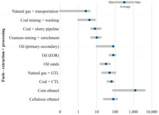
The water footprint argument for gas extraction can also be applied across all energy
production techniques. As Figure 2-3 points out, natural gas extraction and transport requires
less overall water usage than any other fuel extraction and processing (Mielke et al. 2010).
Figure 2-4. Water Usage for Extraction and Processing of Energy Fuels http://belfercenter.ksg.harvard.edu/files/ETIP-DP-2010-15-final-4.pdf.
2.2.4 Contentious Nature of Hydraulic Fracturing
The economic benefit of oil and gas extraction, particularly with the expanded use of
unconventional methods, competes with the desire to protect the environment. With the
lobbyists will not allow environmentalists to prohibit hydraulic fracturing in the near future.
Despite the high likelihood that anti-fracturing groups will not be able to stop fracturing from
continuing, the need for innovations in the handling and treatment of the operations before,
during and after the initial stimulation will be critical items to address going forward.
2.2.4.1 Environmental Issues
Gregory (2011) stated the environmental implications succinctly in his report noting that
one of the challenges will be maintaining the economic feasibility of production while being
responsible for the natural resources and public health that could be effected by oil and gas
operations. Maintaining the environment and public health is an important issue due to the
rapid expansion of tight oil and shale gas using hydraulic fracturing, especially considering the
potential impacts on United States drinking water, both ground and surface, as well as potential
impacts on air quality (Ratner and Tiemann 2015). This issue was pressed further into the
spotlight by the recent publication from the EPA that groundwater is susceptible to
contamination from hydraulic fracturing activities (EPA 2015). However, concerned parties
regularly point out the fact that in 2005, fracturing was specifically exempt from the regulations
under the Safe Drinking Water Act (MacRae 2012). Whether drinking water impacts are rare or
not, or environmental regulations apply or do not, the concern is justified with 25,000 to 30,000
new wells being drilled between 2011 and 2014 (EPA 2015).
2.2.4.1.1 Air Emissions
Air pollution associated with hydraulic fracturing operations has also gained attention as
and include pad, road and pipeline construction, well drilling and completion, produced water
collection and processing, and all phases of refinement, storage and transportation. The main
air pollutants of concern are methane, volatile organic carbons (VOC), nitrogen oxides (NOx),
sulfur dioxide, particulate matter (PM) and various others (Ratner and Tiemann 2015 and EPA
2012). These emissions can react with nitrogen oxides in the air and form ozone. Fort Collins
consistently has a low rating from the State of the Air Report and received an F, with 8.6 more
high ozone days from 2009 (SOTA 2015). This increase in Fort Collins could be caused by
several factors, which includes the increase in fracking in Weld County and other places along
the front range.
2.2.4.1.2 Trucking
Trucking is a large issue for societal and environmental concerns. Transporting the
millions of gallons of water needed for fracturing each well can require roughly 1,500 truck trips
(Boulder County Research 2013 and NTC 2011). The impact of the constant flow of trucks is felt
especially harshly in communities with heavy oil and gas extraction, i.e. many wells located in a
small geographic area. The truck traffic also affects roadways, as the heavy weight of the trucks
at scale could add usage for which the roadway was not designed. The damage could then
result in repair costs and construction traffic delays. Accident rates are also higher, noted as
increasing between 15 and 65 percent, in areas with hydraulic fracturing activity, and fatalities
and major injuries also increased (Graham et al. 2015). The specific air emissions of concern for
2.2.4.1.3 Land issues
Land issues are similar to trucking issues in societal and environmental concerns. The
increase in wells and, therefore, well pads have caused the operations to become closer to land
owners, communities and waterways. The counter argument is that hydraulic fracturing
reduces the amount of well pads overall, a fact supported by many sources including Colorado
Oil and Gas Association (Arthur et al. 2008). However, despite the reduced well pad quantity,
roughly 9.4 million people lived within a mile of a hydraulically fractured well between the
years of 2000 and 2013, roughly 3 percent of the US population. Additionally, that mile radius
around all the hydraulically fractured wells nationwide includes 6,800 drinking water sources
that provide water for over 8.5 million people (EPA 2015).
2.2.4.1.4 Water Issues
With the proximity of the wells to the population and the water sources on which they rely,
the concern over water safety is well founded. Concerns for groundwater contamination
include the development of the well, the drilling through aquifers and the casing surrounding
the well bore, cementing and the completion of the well (Ratner and Teimann 2015). The new
EPA study on hydraulic fracturing risks to drinking water offers a more detailed explanation of
how hydraulic fracturing might impact drinking water (EPA 2015). In the study, the authors
note that cement casing is a critically important feature for protecting aquifers that are drilled
through. The casing, if extended below the bottom of the aquifer, reduces the risk of
groundwater contamination by a factor of 1000. The study furthers explores the potential risk
to ground water through hydraulic fracturing based on depth of the source rock below the
several thousand feet below the aquifer, the likelihood of a fracture travelling through the
overlying rock to the drinking well is low (EPA 2015). However, the likelihood of impact
increases as the source rock approaches the ground surface and aquifers. Potential impacts
increase further when wells are located near each other or near older or abandoned wells. The
proximity of fractured wells could cause intermingling of the fractures created by the multiple
wells. Old and abandoned wells are susceptible due to their design or other reasons, like outdated ell plugs. The pote tial o ta i atio s o f a hits , as the a e efe ed to i the study, suggest that intermingling could affect the well components and result in fluids released
at the surface (EPA 2015). The surface impacts can extend beyond well components failing.
Transporting of produced water usually involves truck traffic and, as noted previously that
traffic accidents increase in fracturing areas, spills can occur. Spills, in reported sites in
Pennsylvania and Colorado, were recorded between 0.4 and 12.2 per 100 wells, with 74% of
those being caused by failing containers (EPA 2015). Spills that migrate to water bodies can
impact the water quality, which is the cause for the concern.
2.3 Water Management and Treatment
With the potential for environmental damage, specifically to water sources, the oil and gas
industry will have to develop practices that mitigate and manage the impacts they might cause
on the surrounding area. This fact is especially pertinent in regards to the o pa ies’ ate management strategies. These water management strategies are developed for several
reasons. In some cases, like Pennsylvania, water management is required by regulatory
agencies. However, in many cases, the water management strategies are developed in
oil and gas production are; sourcing the water used for the fracturing process and treating
produced water. Both the water acquisition and wastewater production require transportation
and the wastewater also requires treatment (Ratner and Tiemann 2015).
If one tries to calculate the initial water needs for the well, assuming 5 million gallons of
water used for stimulating each well, and based on the EPA estimate of 30,000 wells fractured
from 2011 to 2014, then the water needed for fracturing was 150 billion gallons. The sheer
volume of water requires a high degree of coordination for water gathering and delivery to the
well site, as well as treatment and disposal. The usage, though a small percentage of the
overall water usage in the United States, does add to the problem of water scarcity in regions,
especially regions considered to be in high or extremely high water stress. From January 1,
2011 through May 31, 2013, 48 percent of wells were in high or extreme water stress and 56
percent of wells were in drought regions, including 100 percent of the wells in the
Denver-Julesburg basin (Freyman 2014).
Wastewater volume, though lower than the volume used to fracture the wells, also requires
attention. Estimates for oil and gas wastewater production in the United States was 15 to 20
billion barrels per year in 2009, and that number is sure to have risen with the increase in wells
(Clark 2009). Flowback, which typically lasts from one to four weeks after initial flow, accounts
for up to 40 percent of total water that is removed from the well (Arthur 2008). Flowback fluids
have properties similar to the fracking fluid that was used to stimulate the well. As the well
matures, the wastewater becomes less like the fracturing fluid and more of a reaction between
the fracturing fluid and the geologic formation of the source rock and then is termed produced
Barnett Shale is an exception with the produced water equaling or even exceeding the injected
volume (EPA 2015). Either way, all this wastewater from unconventional wells requires
treatment and/or disposal.
2.3.1 Disposal
As the industry has evolved, including during the time dominated by conventional drilling,
companies have experimented with many different methods for disposal. The volume of
wastewater produced creates pressure for the industry to find ways to treat and dispose of the
water in means that are cost effective, and regulatory agencies have attempted to maintain the
effectiveness of the treatment to minimize risks to the public and environment. In Colorado,
produced water is disposed of by three means: underground injection wells (60 percent),
evaporation ponds and discharge to surface water (20 percent for each) (COGA 2011).
2.3.1.2 Publicly Owned Treatment Works (POTWs)
The use of POTWs is an option for disposal of wastewater; however, there are many
constraints that limit the use of this method of produced water disposal. The first limitation
can be the cost. POTWs charge a fee for cleaning the water they receive to pay for operations
and maintenance. However, an even larger limitation is regulations that the POTWs face from
the EPA and state agencies. The main concerns with treating produced water are total
dissolved solids (TDS), oil and grease (Gregory et al. 2011).
2.3.1.2 Evaporation Ponds
Evaporation pond usage, as noted previously, accounts for 20 percent of the produced
water so that the contaminants are left in the pond. The usage of evaporation ponds is only
sustainable if the inflow (produced water and precipitation) is less than the evaporation rate,
which is dependent upon pond size and depth and can be hindered by solids and chemical
levels. Another concern is the attractiveness of the water bodies to birds and other animals,
which would be covered by oil and grease if they land in the pond (NETL Fact Sheet). A final
concern is the air emissions associated with ponds, such as volatile organic compounds (VOCs)
like benzene, toluene, ethylbenzene and xylenes among other volatiles(O&G Journal 2009; EPA
2009).
2.3.1.3 Reverse Osmosis
Reverse osmosis is a process of utilizing a pressure gradient through a membrane that is
semi-porous allowing water to diffuse through while partially rejecting salts and organic
molecules. The pressure gradient separates the water from the contaminant by the filter by
allowing the water particles to pass through while capturing the contaminants behind the filter.
The concentration of the contaminant left behind in the membrane must be disposed of
properly. The contaminants that can be removed include organic molecules and salt ions and
RO is commonly employed in desalination processes (Xu 2006). The water produced from this
membrane separation technique is of high quality; however, the process is very energy
intensive. Any process that is energy intensive will require high operating costs, unless the
energy is cheap to produce, and the cost makes this particular treatment technique
2.3.1.4 Thermal Distillation and Crystallization
Thermal distillation requires evaporation, just like the evaporation ponds, to treat the
produced water and separate the water from the dissolved contaminants. Once the water is
evaporated, a heat exchanger condenses the vapor to produce purified water. It has been
shown that distillation can remove up to 99.5 percent of dissolved solids with the potential to
reduce disposal costs (ALL Consulting 2003). Thermal distillation has the ability to treat
produced water with a TDS up to 125,000 mg/L of TDS. However, this technology is like reverse
osmosis in that it is more expensive than disposing through deep underground injection and
purchasing fresh water for future fracturing (Veil 2008).
2.3.1.5 Deep Underground Injection
Deep underground injection has become the most popular method for disposing of
produced water (Clark 2009). Injection wells are used most often due to the cost of disposal ei g the lo est, ho e e , that ost a i ease due to dista e to the ells’ sites. Additio al constraints on disposal wells are regulations that ban them in several states. The regulations
stem from reports that show the potential for aquifer contamination as well as the potential to
induce seismic activity (Dores 2012). When the method is utilized for disposal, the disposal
occurs in a Class II disposal well (Veil 2004).
2.3.1.6 Beneficial Reuse
Beneficial reuse is another method that oil and gas producers use to dispose of produced
water. This method involves treating the produced water through various treatment
habitat enhancement and on fields for livestock. The advantage of beneficial reuse is the ability
to have a lower standard of treatment as opposed to disposing to a surface water body. The
main concern for water quality is TDS, specifically for sodium, chloride, calcium, magnesium,
iron, barium, boron and strontium (Nijhawan 2006).
2.3.2 Recycling
Another form of beneficial reuse is recycling treated produced water to be used in the
hydraulic fracturing process of a new well. The process of treating the water for reuse can be
much simpler than treating it for disposal or other forms of beneficial reuse. This is due to the
fact that TDS in the produced water can be beneficial for the next well stimulation. However,
high TDS negatively affects fracturing additives like cross-linkers. The use of recycled water
seems to be occurring due to pressure from society or regulations. For instance, in
Pennsylvania, the concerns from citizens and environmental groups and the effects of produced
water in rivers pushed the Pennsylvania Department of Environmental Protection to issue an
order for POTWs to stop accepting produced water. The order, which specifically targeted TDS
effluent to be less than 500 mg/L, along with a geology in the region of the hydraulic fracturing
that was not conducive to injection wells prompted companies to become more creative with
their produced water treatment. One company responded to the inability to use POTWs by
recycling more than 95 percent of its produced water for fracking additional wells (Rassenfoss
2011). And for the industry as a whole, the reuse rates in the Marcellus region have jumped to
2.3.2.1 Drawbacks
The reuse of produced water for future fracturing fluid presents some difficulties.
Bacterial growth and chloride contamination both present safety concerns that producers must
be cognizant of when exposing their employees to the produced water (Vidic 2010). The
bacteria could also be a concern for well-bore integrity, as bacteria can foul a well if it grows in
the well. As discussed previously, the difficulties arise due to chemical reactions. Specifically,
the level of TDS affects the effectiveness of emulsion friction reducers. The effectiveness of the
friction reducers is negatively affected because the high concentration of divalent cations in the
produced water hinders the ability of the friction reducers to invert (Sareen et al. 2014 and
Zhou et al. 2014). The reduction in effectiveness has caused fracturing companies to
experiment with new chemistry.
2.3.2.2 Benefits
Reusing produced water in fracturing future wells has multiple benefits including societal, e i o e tal a d e o o i . The so ietal e efits i lude sho asi g a o pa ’s
o it e t to p ote ti g o u ities a d the o u ities’ esources. If done strategically, recycling minimizes truck traffic and reduces the strain on water sources in the region. As
noted previously, minimizing strain on fresh water is important especially considering the
location of most of the wells in water scarce regions. One economic impact of recycling
produced water is shown by a study by Zhou et al. (2014) in which they measured the
effectiveness of a new friction reducer on a well site in Texas. The friction reducer was tested
with recycled water with a TDS value of 250,000 mg/L and 50,000 mg/L hardness. The results
2.4 Research Purpose and Objective
As unconventional oil and gas plays become more popular, the increase in wells will have a
two-fold i pa t o a egio ’s ate esou es. The i ease i h d auli f a tu i g ill add to demand for fresh water sources and treatment solutions for produced water. It is with these
two concerns in mind that companies need to seriously consider recycling produced water for
fracturing future wells. For the Wattenberg area, companies need to begin gathering data on
the effects of recycling produced water in fracturing. Gathering the data on the differences of
using fresh water versus recycled water will become important when companies determine
produced water treatment strategies.
Little work has been done to understand how different base fluids affect the quality and
quantity of produced water. However, The Colorado State University Center for Energy Water
Sustainability conducted research on fresh water versus recycled wells in Weld County with two
recycled wells and two fresh water wells (White 2014). The recycled well, a seven part fresh
water to one part recycled water, and fresh wells had significantly more samples than the
secondary wells. Figure 2-4 shows the difference in the fracturing fluid used, the vertical depth
and the base water volume of the different fracturing packages used for the wells at Crow
Table 2-2. Crow Creek Wells Compared to Chandler State Wells (White 2014)
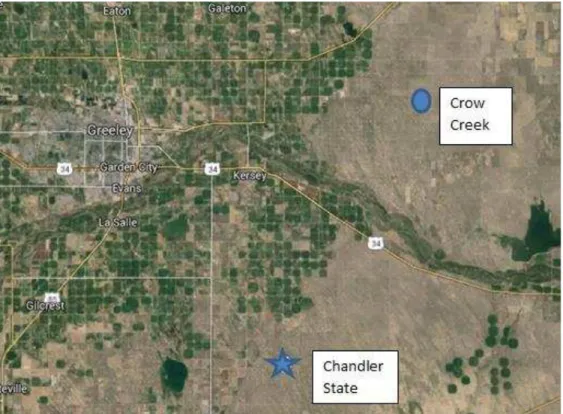
The depths are all similar as is the formation that the wells were targeting. The main
difference is the Fluid Package, PermStim versus SilverStim. A o di g to Halli u to ’s e site, Permstim is a polymer as is SilverStim. Figure 2-5 shows the spatial difference between the two
wells, which is approximately 50 miles. Figure 2-6 shows the Wattenberg Field in the Denver
Julesburg Basin as well as the formations of interest for the oil and gas companies in the area.
Designation Well Name API #
True Vertical Depth (ft) Base Water Volume (gal) RecycleWa ter Vol. (gal) Stages FracFluid Package
Primary Recycled (7:1) Crow Creek State
AC36-73HN 05-123-37423-00-00 6685 2,371,163 296,395 PermStim Primary Fresh Crow Creek State
AC36-76-1HN 05-123-37420-00-00 6742 1,335,328 0 PermStim
Secondary Fresh Crow Creek State
AC36-73-1HN 05-123-37422-00-00 6747 2,403,381 0 PermStim
Secondary Recycled (5:1) Crow Creek State
AD31-79HN 05-123-37426-00-00 6674 2,301,153 383,526 PermStim Chandler State D15-72-1HN Chandler State D15-73-1HN Chandler State D15 74-1HN SilverStim Primary Recycled (5:1) 05-123-383321-00 6840 3,154,662 525,777 23 SilverStim
Primary Recycled (7:1) 05-123-38323-00 6759 3,677,478 459,684 23 SilverStim
Figure 2-5. Map Showing Location Between Crow Creek and Chandler State (Google Maps)
Figure 2-6. Wattenberg Field in the DJ Basin and the Geologic Formation http://www.syrginfo.com/operations/operations-overview.
The Crow Creek data from the sampling showed that the recycled wells had higher early TOC
and turbidity values than the fresh water wells, which is shown in Figure 2-7 and 2-8,
respectively.
Figure 2-7. TOC Comparison (White 2014)
73HN and 79 are the two recycled wells. Well 79 was used as a check of the data and
only has 5 days of sampling, but does appear to verify the results found in Well 73HN. The
same sampling method was used for 76-1 and 73-1. Looking at wells 73HN and 76-1, the TOC
value is higher in the early sampling period in the recycled well.
Figure 2-8. Tubidity Comparison
Similar to the data from the TOC measurements, the turbidity is higher in the recycled
well in the first 14 days. The TOC of the e led ell’s p odu ed ate e ai s t i e as la ge as the f esh ate ell’s p odu ed ate th ough da ith alues of , a d , ,
espe ti el . B da , the f esh ate ell’s TOC is , a d the e led ate ell’s TOC is
0 2,000 4,000 6,000 8,000 10,000 12,000 0 20 40 60 TOC (m g /L) Time (days) 73HN 79 500 1,500 2,500 3,500 4,500 5,500 6,500 0 20 40 60 TOC (m g /L) Time (days) 76-1 73-1 0 10,000 20,000 30,000 40,000 50,000 0 20 40 60 Tu rb id ity (N TU ) Time (days) 73 79 0 20 40 60 Time (days) 76-1 73-1
1,526 indicating that the impact of the recycled well does not last throughout the sampling.
Both also appear to be become similar near day 20 around with turbidi. This difference in the
early period of the sampling led to the belief that the recycled base fluid impacts the produced
water quality, especially the organic difference.
The wells studied in this thesis were chosen by Noble to verify the data found in the Crow
Creek Wells. The purpose of this research is to utilize laboratory methods to measure the
organic and inorganic content and LCMS data to analyze produced water samples to gain a
better understanding of the difference between the recycled and fresh water base fracturing
fluids. The objectives of this research were:
Collect produced water samples from three wells in the Wattenberg field. The three wells will allow us to compare differing levels of recycling in hydraulic fracturing
fluids. The first well will use all fresh water, the second will use 1:5 recycled/fresh
water and the last will have 1:7 recycled/fresh water.
Perform laboratory methods, both in house and through a state certified analytical laboratory, to measure different organic, inorganic and LCMS data from the samples
collected to measure if there are temporal differences in the samples.
Utilize laboratory techniques to analyze the samples to better understand how the different fracturing fluids affect the quality of the produced water.
3 WATER QUALITY CHARACTERIZATION
3.1 Introduction and Purpose
Analysis of produced water quality from wells fractured with recycled water has not
been analyzed to any great degree and then compared to wells fractured with fresh water.
Understanding of the effects of recycled water may impact treatment strategies should a
difference be found between produced water quality in fresh and recycled wells. This is
especially important for oil and gas companies whose current water management strategy, like
the operators in the Wattenberg field, has been developed for fresh water wells.
The objective of this study was to measure the water quality from the three wells based
on organic and inorganic constituent characterization to answer several questions about the
possible differences caused by using recycled water in the fracturing fluid. The questions
analyzed are the following:
Is there a statistical difference in organic constituents found in the produced waters? Is there a statistical difference in inorganic constituents found in the produced waters? Do the organic and inorganic constituents in the produced water change temporally? What effect might the potential differences have on water management strategy? 3.2 Fracturing Fluid
Table 3-1 displays data gathered from FracFocus.org about the composition of the
fracturing fluid. The table shows the similarities of the fracturing fluid make up. The largest
difference in the ingredients is friction reducer, breaker, buffer and cross-linkers. These
research group has shown that small changes in the fracturing fluid can have large effects on
the water chemistry of the produced water (Sick 2014).
Table 3-1. Fracturing Fluid Composition As Found On FracFocus.org
The difference in the friction reducer can be explained by the use of recycled water. Recycled water has a higher TDS, which can minimize the effectiveness of friction reducers due to the divalent cation content of the recycled water. Table 3-2 displays the TDS data from the three fracturing fluids. For Well R1, the data corresponds to the theory that the friction
reduction would be affected as they had to use nearly double the amount of friction reducer as the Well F, but it does not follow for Well R2 where half the friction reducer was required than Well F despite a much higher TDS.
Purpose Trade Name Ingredients
Well F Max Conc. (% by Mass)
Well R1 Max Conc. (% by Mass)
Well R2 Max Conc. (% by Mass)
Base Fluid Fresh Water Fresh Water 85.5 76.4 N/A
Base Fluid Recycled Water Recycled Water 0 10 N/A
Proppant Sand - Premium
White Crystalline silica, quartz 13.6 12.7 13.86
Gelling Agent WG-18 Gelling
Agent Guar gum derivative 0.2 0.2 0.1
Sodium chloride 0.1 0.1 0.03
Chlorous acid, sodium salt 0.03 0.03 0.1
Potassium carbonate 0.06 0.1 0.04
Isopropanol 0.04 0.03 0.01
Surfactant OilPerm FMM-2 Citrus, extract 0.01 0.1 0.02
Triethanolamine zirconate 0.02 0.02 0.01
Glycerine 0.005 0.005 0.01
Propanol 0.005 0.005 0.01
Additive Cla-Web Ammonia Salt 0.01 0.01 0.01
Activator CAT-3
ACTIVATOR EDTA/Copper Chelate 0.009 0.009 0.01
Zirconium, acetate lactate
oxo ammonium complexes 0.005 0.005 0.01
Ammonium Chloride 0.003 0.003 0.01
Friction Reduction FR - 66 Hydrotreated light
petroleum distillate 0.004 0.007 0.002
Activator CAT - 4 Diethylenetriamine 0.003 0.003 0.003
Buffer Breaker Vicon NF Breaker CAT-3 CROSSLINKER Crosslinker Crosslinker CL-37 Crosslinker BA-40L Buffering Agent
Table 3-2. Total Dissolved Solids in Fracturing fluids
In this study, the fracturing fluid is anticipated to be the largest contributor to the
quality of the produced water due to the age of the well during the sampling period. Typically,
the water coming out of a well will have more similarities to the fracturing fluid early in the ell’s life le a d ill shift o e ti e to e a o i atio of the f a tu ing fluid and any compounds and elements that might have interacted with the fluid. However, the fracturing
fluids influence on the water coming out of the well can last for weeks after the fracturing
process is complete and the well is already producing.
3.3 Sample Collection
Nineteen samples were collected at the Chandler State well site over a 36-day period.
The sampling began the first day of oil and gas production and was gathered directly from the
well-head, which is a potential reason why the day one data shows discrepancy. The rest of the
samples, which occurred every day for the first 14 days, then every three days until day 29 with
the final sample taken on day 36, were taken from permanent separators, which separate much
of the oil from the water coming out of the well. Each well has its own separator, which
allowed for measuring each individual well. For work performed in the CSU laboratory, a one
liter bottle was filled for sample testing, including the pH which was taken at the well site, as
well as 2 volatile organic analysis (VOA) glass vials for liquid chromatography mass Fresh Recycled Fresh Recycled Fresh Recycled
TDS (mg/L) 1445 n/a 1305 30389 870 23521
Gallons (MG) 3.39 0 3.22 0.46 2.63 0.53
Total Gal
Total TDS (mg/L) 1445 8001 6233
Total Dissolved Solids in Fracturing Fluid
Well F Well R1 Well R2
spectrometry (LC-MS) testing. For eAnalytics, a 250 mL container and two additional VOAs
were filled. The VOAs were all filled so that there was no air space when the cap was placed on
the VOA.
3.4 Methods
3.4.1 Analysis Performed at CSU
The following tests were performed at Colorado State University.
3.4.1.1 Gravimetric Solids Analysis and Turbidity
Solids were measured using gravimetric solids analysis and turbidity. Gravimetric solids
analysis was utilized to determine the TS, TSS, TDS, TVS, VDS, VSS and the tests were performed
in accordance with Standard Methods, Method 2540. All the tests utilized weighing to measure
the solids. For TS, a sample is weighed and put into the oven at 105 degC for drying and is
reweighed after drying. For TSS, a sample is poured over a Whatman 934-AH
1.5-um-equivalent pore size glass microfiber filter. The filter is then placed in the 105 degC oven for
drying. The TDS sample is collected from the collected water after filtering. It is also placed in
the 105 degC oven for drying. For the volatile testing, the same procedures are followed for TS,
TSS and TDS but the samples are placed in the 550 degC oven to mineralize the organics and
can be used to estimate the organic loading in the produced water. Turbidity, which is a
measure for colloidal solids that have a strong impact on light reflection, was measured using a
HACH 2100 N turbidimeter. The device reads the light refraction in nephelometric turbidity
3.4.1.2 TOC and DOC
TOC and DOC were both analyzed using a Shimadzu TOC-VCSH analyzer. This analyzer
determines the TOC by finding the difference between total carbon and total inorganic carbon.
The two amounts are measured when carbon in the sample is oxidized to CO2. For TOC, the
sample is taken directly from the well samples, then diluted at a ratio of one (1) to 10. For the
DOC, the same process for TDS and VDS is utilized and the sample for DOC is gathered after
filtering through a 1.5-um-equivalent Whatman 934-AH glass microfiber filter.
3.4.1.3 pH , Alkalinity, Carbohydrates
pH was measured on site using HACH probes using CDC401. For alkalinity, Standard
Methods 2320B was used for measurement. The Carbohydrate method is described in detail in
Appendix D.
3.4.1.4 LC-MS
Testing the samples using LC-MS was performed less frequently than the other samples
in this study. The sample days chosen for LC-MS testing was days 1, 2, 6, 10, 14, and 20. The
test uses Agilent 1290 series liquid chromatography with Agilent 6530 quadrapole time of flight
(QTOF) that has Electrospray Ionization of positive and negative modes. 12 L/min was provided
for shear gas flow with a temperature of 400 degC. The nebulizer pressure was 30 psig. The
regular gas flow was also 12 L/min but with a temperature of 325 degC. The voltages were 750,
60, 120 and 500 V for the octopole RF peak voltage, skimmer voltage, fragmentor voltage,
nozzle voltage, respectively. The mobile phases were 0.1% formic acid in water for A, 0.1%
95-80% of A for 1-8 minutes, 80-5% of A for 8-17 minutes and 5-95% of A for 17-18 minutes.
Mobile phase B makes up the remaining portion of the fluid in the gradient.
Due to the limit of chemical standards, the qualitative analysis of the organic
compounds was performed by searching the library in Agilent Technology Software based on
the exact mass of the chemicals used for hydraulic fracturing in U.S (Chemicals Used in
Hydraulic Fracturing 2011). A 5 ppm mass accuracy was applied for detection of chemical
compounds.
3.4.2 Analysis Performed by eAnalytics
eAnalytics is the lab outside of CSU that was contracted to perform several tests on the
samples. The tests included determining the content of metals, ammonia (NH4), bicarbonate
(HCO3), bromide (Br), chloride (Cl), sulfate (SO4), gasoline range organics (GRO), diesel range
organics (DRO), oil range organics (ORO), total petroleum hydrocarbons (TPH) and benzene,
toluene, ethylbenzene, and xylenes (BTEX). The method for determining the metals, aluminum
(Al), boron (B), barium (Ba), bromine (Br), calcium (Ca), iron (Fe), potassium (K), magnesium
(Mg), sodium (Na), silicon (Si), strontium (Sr), zinc (Zn), chlorine (Cl), was EPA 6010C that
involves adjusting the pH to below 2 and using inductively coupled plasma-atomic emission
spectrometry (ICP-AES). Ammonia was determined using EPA 350.1. Bicarbonate
dete i atio used EPA . . B o ide’s ethod as EPA . . Chlo ide’s ethod as EPA 9253. Sulfate utilized ASTM D516. GRO, DRO, ORO used EPA methods 8260C, 8015, and 8015
3.4.3 Data Analysis Techniques
To understand the data and see any correlations or similarities, this study uses analysis
of variance (ANOVA) testing. The ANOVA assumptions include normally distributed and
homogenous variance. The Box and Whiskers (in text and Appendix F) show skewed
distributions, but due to a small size ANOVA was still used. ANOVA testing is a statistical
analysis approach that can be used to measure the difference between two or more data sets.
The equation used for the ANOVA method is listed below in Equation 1.
Yi= µ + αt + βj + αtβj + εij (1)
In Equation 1, Yi is the variable under investigation. µ is the overall mean and is used to
characterizing the mean value, but is not well or time dependent. α is the a ia le that represents ea h ell a d β is the ti e o po e t. αtβj represents the intercept of the wells but can be eliminated if the p-value is less than 0.05, which is the designated value for
determining statistical difference. The ANOVA method outputs a p-value that corresponds to
either the hypothesis being acceptable (usually p<0.05). If the p>0.05, then the alternate
hypothesis is correct. The alternate hypothesis is that the recycled wells are significantly
different, and the null hypothesis is the wells are not significantly different. ANOVA uses linear
regression to determine the similarities in the data sets and can be seen in equations 2 through
5.
Ho: α1 = α2 = α3 (2)
Ho: β1 = β2 = β3 (4)
HA: β1 ≠ β2 ≠ β3 (5)
Equations 2 and 3 indicate the null hypothesis that the wells do not show a statistical
difference and the alternate hypothesis is that they are statistically different. The ANOVA tests
whether there is a difference in well chemistry. Equations 4 and 5 shows the same statistical
test but for the wells over time. For the time portion of the ANOVA results, the method takes
an average of the data points in that time period. The time periods are broken down into three
groups. The first time group is days 1-7 and is labeled as early time period. The second time
period groups days 8-13 and labeled as middle time period. The third time period includes days
14-29.
A simple linear regression model was used to estimate similarities of produced
water quality (Eqn.6) between each recycled well and the fresh water well. This linear
regression was used as another method for inorganic data analysis.
Y = β +β X (6)
In this model, dummy variable D and D were used, which were both set to 0 if the water quality parameters come from Well F, D was 1 and D was 0 if the data came from the water quality parameters from Well R1, and D was 0 and D was 1 if the data came from the water quality parameters from Well R2. That is,
{
D = andD = , ifdatacomefromWellF D = andD = , ifdatacomefromWellR D = andD = , ifdatacomefromWellR
(7)
By combining Equations (6) and (7), the following equation is obtained:
Y = β +β X+ β + β X × D + β + β X × D (8)
Where β , β , β , β , β and β are fitting coefficients and D and D are dummy variables. Three different equations were acquired based on the ratio of fresh water and
recycled water used:
YwellF= β +β X (9)
YwellR = β +β + β + β X (10)
YwellR = β +β + β + β X (11)
The null hypothesis for the linear regression model was that coefficient βi is zero and the alternative hypothesis was that βi is not zero. Coefficients β , β are fitting constants for Well F, coefficients β , β are fitting constant for Well R1 and coefficients β , β are fitting constant for Well R2. Coefficients β and β indicate a statistically significant difference between Well F and Well R1 and coefficients β and β indicate a statically significant difference between Well F and Well R2. Relatively lower values for the coefficient of
were not strongly related. For wells having the same y-intercept means the fresh water well
and the recycled wells have the statistically similar starting values at time equals zero, which
might indicate that the ratio or recycled to fresh water does not affect the constituent in
question. If the slopes are same, then that could indicate the wells are affected by the
geological formation at the same rate.
3.5 Results
This section will detail the results of the analysis on the produced water samples taken
from Well F, R1 and R2. The data will be presented in graphs, the ANOVA results and the other
statistical method utilizing linear regression. The data will be presented as figures in this
section or in Appendix B.
3.5.1 Gravimetric Solids and Turbidity
Table 3-3 displays the minimum, maximum and average for TS, TDS and TSS. Figure 3-1
shows box plots for TSS, TDS and TS. Figure 3-2 below provides the temporal data for TSS, TDS
and TS. It begins at day one of sampling and continues through day 29.
Table 3-3. Total Solids for All Three Wells Sampled
Well F Well R1 Well R2 Well F Well R1 Well R2 Well F Well R1 Well R2
Min 9,020 12,900 14,920 12,960 12,880 14,420 48 44 129
Max 17,260 18,820 40,060 23,080 17,960 22,840 1,229 532 500 Average 15,139 16,696 19,562 15,354 16,189 17,887 362 230 236
Figure 3-1 clearly indicates that the TS is mainly influenced by the TDS of the samples
due to the large difference in concentrations in the samples. For TSS, the Early Time Period has
the largest ranges and maximums for all the wells. This type of variation was seen in the data
from Crow Creek as well. The ranges and maximums decreased over time and was the smallest
and had the lowest maximum concentration in the Late Time Period. For TDS, Well F had the
largest range between its first and third quartile in the Late Time Period. The TDS was very si ila i a ge a d edia du i g the Ea l a d Middle Ti e Pe iods, a d the ells’ edia
alues e e i the sa e o de du i g all th ee ti e pe iods. The o de of the ells’ edia values was the same for the Early and Middle Time Periods, but flipped for the Late Time