Money Supply Behavior in
‘BRICS’ Economies
- A Time Series Analysis on Money Supply Endogeneity and Exogeneity
Bachelor’s thesis within Economics
Author: Pengcheng Luo
Supervisors: Pär Sjölander Kristofer Månsson
Bachelor’s Thesis in Economics
Title: Money Supply Behavior in ‘BRICS’ Economies
Author: Pengcheng Luo
Tutor: Pär Sjölander, Kristofer Månsson
Date: November 2013
Keywords: Money Supply, Monetary Policy, BRIC, BRICS, Emerging Economy, Endogeneity, Exogeneity, Monetary Targeting, Time Series, VAR, VECM, Granger Causality, Monetary Economics. JEL classification: E12 E42 E50 E52 G21 G32
Abstract
In this thesis the money supply behavior of the ‘BRICS’ group is investigated from 1982 to 2012. It is empirically analyzed whether there are causality relationships between related monetary indicators by using quarterly data and time-series econometrics methods. In four countries: Brazil, China, Russia (the period of 2004-2012) and South Africa (1982-1993), this study found money supply endogeneity evidence. Thus, this implies that bank loans cause the money supply, or that there is bidirectional causality between these two. Regarding the other countries (India and the 1982-2003 period of Russia) money supply was found to be exogenous, i.e. money supply cause bank loans. Nonetheless, the traditional monetarian view still holds across the five economies in the short run. The findings reflected discretionary monetary policies targeting monetary aggregates in the short term, despite a neutral role of most central banks in the long run.
1
Table of Contents
1
Introduction ... 3
1.1 Proposed Questions ... 4
1.2 Limitation and Organization of this Thesis ... 5
2
Theories and Earlier Studies ... 6
2.1 History of Endogenous vs. Exogenous Money ... 6
2.2 Three Money Supply Determination Approaches ... 8
2.3 Previous Studies ... 10
3
Data and Variables ... 11
3.1 Data Source ... 11
3.2 Variable Definition ... 12
4
Econometrics Method and Preliminary Results ... 13
4.1 Chow Breakpoint Test ... 13
4.2 Unit Root Test ... 16
4.3 Johansen Cointegration Test ... 19
4.3.1 Lag Determination ... 19
4.3.2 Cointegration Test ... 20
4.4 Causality Tests ... 21
4.4.1 Standard Granger Causality Test ... 21
4.4.2 VECM ... 22
4.4.3 Trivariate VAR ... 23
5
Results and Discussion ... 24
5.1 Results in Previous Section ... 24
5.2 Cointegration Results ... 24
5.3 Causality Test Results ... 26
5.3.1 VECM Results ... 29
5.4 Trivariate VAR Results ... 31
5.5 Conclusions ... 33
5.5.1 Discussions ... 34
5.5.2 Policy Implications ... 35
5.6 Suggestions for Further Study ... 36
6
Acknowledgment ... 37
7
List of references ... 38
2
Index for Tables, Equations and Figures
Table 4.1 Chow Test ... 15
Table 4.2 Phillips-Perron Test ... 17
Table 4.3 Optimal Lag Length for Johansen Cointegration Test ... 20
Table 5.1 Johansen Cointegration Test ... 25
Table 5.2 Granger Causality test ... 27
Table 5.3 Vector Error Correction Model ... 29
Table 5.4 Relationship b/t Money Supply and Loans ... 30
Table 5.5 Trivariate VAR ... 32
Table 5.6 Causality Directions... 33
Table 5.7 Conclusions ... 33
Table 8.1 Appendix - Data Source ... 46
Equation 3.1 The Money Multiplier ... 12
Equation 4.1 Vector Autoregressions (VAR) Model ... 19
Equation 4.2 Granger Causality Test ... 22
Equation 4.3 Vector Error Correction ... 22
Equation 4.4 Trivariate VAR Matrix ... 23
Figure 2.1 Brief Summary of Money Supply Theories ... 8
Figure 2.2 Different Money Supply Curves ... 9
3
1
Introduction
This study intended to examine whether the money supply is endogenous or exogenous and how the supply behaves in the so-called ‘BRICS’ economies (Brazil, Russia, India, China and South Africa). By conducting time series analysis on major monetary indicators from 1982 to 2012, money supply endogeneity is witnessed in Brazil, China, Russia (the period of 2004-2012) and South Africa (1982-1993). In other words, of these countries, bank loan Granger cause the money supply, or there is bidirectional causality found between bank loans and money supply. In contrast, in Russia’s 1982-2003 period and India, exogenous evidence has been found, i.e. money supply Granger cause bank loan. However, in the short term, Monetarian view were observed across the five countries, which reflects the discretionary actions taken by the central banks to target the monetary aggregates.
‘BRIC’ is an acronym used by economists referring to the group of four major developing countries: Brazil, Russia, India and China. A Goldman Sachs economist Jim O’Neill (2001) originally created it by taking the initials of the quartet, which makes a heterography of the word ‘brick’. However, it is more than just a wordplay- this group has a total foreign reserve valued at US$ 4 trillion and a combined nominal GDP of more than US$ 16 trillion (IMF data 2012, with the comparison of US GDP the same year: US$ 15 trillion). Furthermore, the developing world is still experiencing undergoing high growth rates in terms of GDP, labor force, and consumption potential. In the meantime industrialized countries are going through near-zero growth. Goldman Sachs forecast ‘BRIC’ group would overtake the developed world as the wealthiest states by 2050. Consequently, it becomes crucial to understand the economic behavior and effects of the emerging economies. In 2010. ‘BRIC’ group has evolved into ‘BRICS’ with the inclusion of South Africa. Continuous studies have devoted into the ‘BRICS’ group, but few in the field of monetary economics. This paper made some modest effort to examine the money supply behavior of the five countries in the last three decades (from 1982 to 2012).
Conventional doctrine has been holding the conviction of exogenous money supply. It claimed that monetary authority determines the money directly. The monetary authority (i.e. central banks) can use fiscal and monetary policies to influence the money supply within a society. The money, then, via the transmission channel (of the IS-LM model) could eventually affect the real economy (Friedman & Schwartz, 1971). It is still widely accepted today, some economists such as Taylor (2009) even argues that this view has escalated during the 2007 Global Financial Crisis. Pro-Monetarism economists have disputed that money exogeneity provided the theoretical foundation for central banks to intervene directly into the money market. Most central banks around the world have reflected this opinion during the crisis time. For instance, during the 2007 crisis aftermath, massive monetary easing policies targeting the money supply directly have been taken by central banks around the world, in the hope of that exogenous money creation could save the economy (Bernanke et
4
al., 2004). The exogenous view of money and Monetarism actions1 have fueled furious
political debates and economic discussions (Krugman 2011, Pethokoukis 2013).
In opposition, unorthodox theory such as Post-Keynesian believes money supply is endogenous with the proposition that money supply is determined within, by the demand for credit and banks’ supply of loans (Lavoie, 1984). Despite growing number of literatures supporting money endogeneity in the industrialized countries, few has yet examined how money supply behaves in the under-developing world. Partially because that the concept of ‘BRICS’ is relatively new. Additionally, due to the prejudice that policies in such countries are highly decisive by the governments rather than markets, thus would understandably support exogenous money supply (Wade and Bruton 1994, Dinç 2005). As the sign of US QE taper finally in sight (Bloomberg, 2013), new sequence of debates of the money supply occurs. This paper takes vision into the ‘BRICS’ states to see which, if any, evidence could support the various money supply theories.
Previous research has provided inspirational insight and firm foundation on the topic. However, the studies were with some limitations: most of the studies have only concerned on a single country; secondly, relatively contemporary data were not available at time the researches were done. Taken these into consideration, innovative contribution of this paper includes: i). The target country expanded to a group of five emerging economies across continents; ii). It has included 30 years of quarterly data; iii). It has taken control of the time-series data problems and potential structural break. Moreover, works such as Badarudin et al. (2013), had taken a pro-endogeneity standpoint prior to the study, then tried to find evidences to accept endogeneity hypothesis. Another improvement of this paper is to take no pre-set bias, to test both endogeneity and exogeneity fairly. Lastly, this paper also included an attempt to identify the impact channel for such monetary policy. Of course, only “standing on the shoulders of giants” makes this study possible.
1.1
Proposed Questions
Under this background, the main objective is to examine whether the ‘BRICS’ countries’ money supply is endogenous or exogenous. In endogeneity theory, the direction of money should be from the bank loans to bank deposits then to the money supply. Meanwhile, as exogeneity theory has shown exogenous money supply has the opposite direction, i.e. from deposits to bank loans. To that end, there are four research questions must be answered:
Research question 1: Does bank loans cause monetary base; do bank loans cause the
money supply? (By the definition monetary theories, exogeneity of the money supply
1 Traditional ways such as reserve ratio and open market operations, which target the interest rate, indirectly
influence money supply. Quantitative easing policy, on the hand, directly targets the supply. Both are reflecting the belief of money exogeneity.
5
should have the causality direction from supply to bank loans only; meanwhile, endogeneity: from bank loans to supply or bidirectional of supply and bank loans). In order to investigate influence channels, the following three questions:
Research question 2: Is there any causality between money supply and national income
(defined as real GDP)? What is the causality direction?
Research question 3: Are there bidirectional causality or not between bank loans and the
monetary multiplier? Is there bidirectional causality between bank loans and supply?
Because that Granger causality is limited to pairwise test, that in order to provide more accurate and detailed results, the following question 4 is proposed. Detailed causality directions and corresponding theories regarding the research question 4, are available in table 5.6 on page 33.
Research question 4: Does the trivariate causality exist: loans cause deposits and deposits
cause the money supply? Alternatively, any other directions?
Through hypothesis tests, conclusions could be drawn for: has money supply endogeneity or exogeneity been witnessed in ‘BRICS’ countries? Which transmission mechanism are the evidence suggests? The theoretical ground for these research questions is detailed in the following section 2. Results and discussions are in the section 5, starts on page 23.
1.2
Limitation and Organization of this Thesis
Due to limitations of the data availability, for example Russia (most data for Russia only available after 1996), China (data for domestic loans only available after 1997) and Brazil (most data for Brazil only available after 1994). As a result, some results may be inconclusive, and in few cases, some degree of inaccuracy could emerge.
In the sections to come, this paper is organized as follows: Firstly, in section two, this part presents a brief review of main theories of monetary economics, followed by literature review of previous studies. Next part of the thesis outlines a description of the empirical data source this study used. Section 4 details the econometrics methodology the thesis would carry out. The empirical findings and conclusions finally present in the section 5.
6
2
Theories and Earlier Studies
2.1 History of Endogenous vs. Exogenous Money
When the topic is concerning monetary economics and monetary policy, conventional Keynesian model would inevitably be brought up. The IS/LM model Keynes proposed (Blinder, 2008) defines the relationship of aggregate demand and employment to two exogenous variables: money and the state budget (money supply curve is vertical). As Wray (1992) defined, the term ‘exogeneity’ is “…in the control sense … government policy is the primary determinant of its value”. Keynesian view (Keynes, 1930 & 1931) rejected neutrality of money both in the short term and in the long term, argued for the monetary policy to keep full employment. (Keynes, 1971, ‘collected writings’ vol.13). His IS/LM model2 provided
exogenous foundation of pro-interventionist view on monetary policy and fiscal budgeting. As the main opponent of Keynes, Hayek (1950) was mainly against the adoption of Keynesian policies (including monetary policy), he argues for the neutrality of money in the long run. Despite the fact that Hayek opposed Keynesian monetary policy citing chronic inflations and mismatch of demand and labor. Nonetheless, he conceded that the monetary policy could be effective- only in the times of widespread unemployment (Hayek, 1967). Wapshott (2012) concluded that Keynes and Hayek had relatively less fundamental disagreement on the topic of money supply’s effects on real economy.
Similarly, Friedman (1956), who is also an advocate opposing Keynesianism, who developed Monetarism view of money, believes that by controlling the money supply, central banks can smooth recessions. Monetarists claimed that exogenously created money is critical in the economic transmission mechanism. They believe that a “helicopter drop” of money into the economy, which central banks can control the quantity of money supply directly (Fridman 2008). More money supply (i.e. liquidity) means banks would lend out more to the public, thus exogenously created money can stimulate investment and consumptions (Phelps, 1990; Bernanke and Reinhart, 2004).
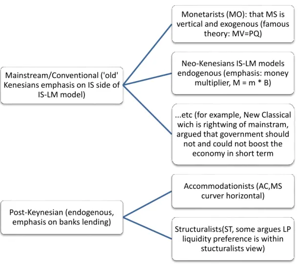
Besides these three widely acknowledged ideologies mentioned above, later on in the history each of their own advocates has advanced with more in-depth and long-lasting debates (Blinder 1988). On one side: the long-holding orthodox school vision of exogenous money supply: so-called mainstreams, such as New Keynesian, Monetarian and Neoclassical Schools. They share the conviction that the causality should run from the money supply to loans. On the other side, challengers like Post-Keynesian, embraces the opinion of endogeneity of the money supply.
The representative of such challengers to conventional monetary theory is the Post-Keynesians (or P-K Economics). Their concept differed from the IS/LM model with the objection of the ‘helicopter drop’ of money and the role monetary multiplier in the supply
2 The LM curve: money supply M = L (liquidity preference, or money demand), which is a function that is
7
process (Palley 1994 & 1998). Instead, P-K economists argued that monetary authority has little or no influence over money supply. Secondly, the money supply responds to the credit channel, which is determined by credit creation of commercial banks’ collective decisions and by the public’s demand of loans (Davidson, 2002; Palley, 1994). Further, they argued, the credit created would cause more deposits, and deposits in turn would create more loans under endogenous supply process (Davidson, 2003).
It is in stark contrast to the supply-side economics (such as Austrian School), which takes "value of money" target; that because money is determined by demand for credit; hence, the causality is from loans to money supply via bank deposits; as a result, the money supply curve should be horizontal or slightly positively sloped. They consider that policies taken by Monetarists and others are causing disequilibrium of the value adjusted automatically by market (supply of loans and demand deposit).
During more contemporary time, the P-K Economics ideology was actually adopted by many monetary authorities. Central banks are in general maintaining neutral role on money supply, only targeting the interest rate as an indirect policy instrument during fluctuations during business cycles (Davidson, 2003; Bernanke and Gertler, 1995). Nevertheless, unordinary quantitative easing measures (‘injecting money’) targets money supply directly have been taken in crisis. This combined picture of long term neutrality and short term ‘crisis mode’ has in fact reflected Hayek’s belief on the monetary policy’s effectiveness in times of widespread unemployment (Hayek, 1967), conventional money exogeneity view, and the quantity theories of exogenously money creation (Friedman 1971) and eventually long term endogeneity of money supply (Davidson, 2003).
8 Figure 2.1 Brief Summary of Money Supply Theories
Reference: “Money Supply: Endogenous or Exogenous” (Snowdon & Vane, 2002) and Dylan Matthews (2012).
2.2
Three Money Supply Determination Approaches
Even with the camp of endogenous money supply, there are different research approaches in terms of the transmission channel. Palley (1991, 1994, and 2013) summarized three main approaches: accommodationists, structuralists and liquidity preference (Figure 2.1 and the following figure 2.2 provided a brief summary3).
3 Panagopoulos & Spiliotis (2008) have gone with even more in-depth, summarized four orthodox and four
Post-keynesian monetary sub-theories. Mainstream/Conventional ('old' Kenesians emphasis on IS side of
IS-LM model)
Monetarists (MO): that MS is vertical and exogenous (famous
theory: MV=PQ)
Neo-Kenesians IS-LM models endogenous (emphasis: money
multiplier, M = m * B)
...etc (for example, New Classical wich is rightwing of mainstram, argued that government should not and could not boost the
economy in short term
Post-Keynesian (endogenous, emphasis on banks lending)
Accommodationists (AC,MS curver horizontal)
Structuralists(ST, some argues LP liquidity preference is within
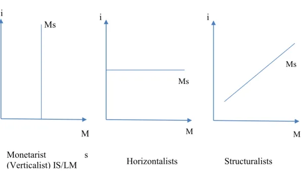
9 Figure 2.2 Different Money Supply Curves4
Reference: “Money Supply: Endogenous or Exogenous” (Snowdon & Vane, 2002), “Endogenous and
Exogenous Money” (Desai, 1987).
1. Accommodationist5 (in abbreviation: AC, also known as the Horizontalists, implying
the horizontal supply curve). As Moore (1998) suggests that money supply is driven by credit: loans cause deposits and in turn, this creates money supply. Central bank is unable to control money supply directly, only the commercial banks fully accommodate any demand for credit at any level of interest rate, but CBs can do short-term adjustment via interest rate manipulation.
2. Structuralists (ST in short; upward sloping supply curve. Main advocates: Pollin 1991 & Palley 1994). Compare to the former accommodationists, the main disagreement is that structuralists argued banks not necessarily fully accommodates. Rather, they emphasis on bank sector’s choice from assets and liabilities assessment when facing an increasing demand for loans, for example, the banks would assess risks, would find the cheapest sources of financing. (Accommodationists and structuralists differ from each other on loan accommodation: the former, on CB’s rate, the latter, on banks’ own initiatives).
4 More detail: Moore, Basil (1988). Horizontalists and Verticalists: The Macroeconomics of Credit Money,
Cambridge University Press; On IS-LM and Monetarism, Bordo and Schwartz (2003).
5 Alternatively, Palley (1994) named them as: pure loan demand approach, mixed portfolio-loan demand
approach, respectively to accommodationist and structuralist view. Ms Ms Ms i i i M M M Monetarist s
10
3. Liquidity preference view (LP, in abbreviation). Dow (1989) sees liquidity preference is within structuralists view. Others (such as Bibow, 2009) argues that banks and other economic agents may prefer liquid assets to illiquid ones. This preference, would then affect behavior of privates, banking sector, and the central banks. Howells (1995) and Moore (1998) explained for example, that after an increase in credits, might not result in a proportional rise of deposits, people’s liquidity preference may transfer part of deposits to more liquid cash.
2.3
Previous Studies
As mentioned in the introduction section, previous studies within this field concerned mostly on the advanced economies, for instance, on G7 economies, Howells & Hussein (1998), Badarudin (2013): both studies found evidence of endogeneity of money supply. Panagopoulos & Spiliotis (2008) also investigated the G7 and they concluded that the seven countries fit differently on monetary theories, but share the common feature of endogeneity. Their study also put that the money multipliers in the G7 group, “are not so effective”. Carpenter & Demiralp (2012) draw similar conclusion for the G7. Moreover, Keen and Grasselli’s test (2012) results in money supply endogeneity for the EU-16 countries.
Despite the overwhelming endogeneity of money supply in the developed world, Switzerland, however, is an exception. Fischer (1993) confirmed the money supply is exogeneity in Switzerland, a country that is known for continuous control over its money: Swiss National Bank (SNB) sticks to tight monetarist actions. It appears that other advanced economies with smaller size are also found exogenous, Altunbas et al (2002), using data 1991-1999, found exogeneity evidences in the countries of: Austria, Belgium, Finland, France, Germany, Ireland, Italy Luxembourg, Netherlands, Portugal, and Spain. Guender (1998) found New Zealand’s exogeneity using data from 1965-95.
There is also research on other parts of world. Some researches were limited into single country. For example, Haghighat (2011) found Iran is consistent with Post Keynesian theories of money endogeneity. Nell’s (2000) analysis on South Africa (1966-1997), concludes money supply in South Africa was endogenous. On Malaysia Shanmugam et al. (2003) has endogeneity findings contradicting with a previous study by Tan and Baharumshah (1999) which found money was non-neutral in short-run, supporting the new Keynesian view). On Croatia: neutral in short run (Erjavec and Cota, 2003). Russia: Vymyatnina (2006) found evidence for accommodationist and structuralist approaches for the period of 1995-2004. Badarudin et al (2009, 2013), found out endogeneity evidences across G-7 countries and five emerging economy, but money found to be exogenous in Mexico, few other developing countries have posted non-concluding results. Based on the methods and theories of these studies and various theoretical sources such as “Handbook of
Monetary Economics” (Friedman et al., 1990), made this study possible to take a modest effort
11
3
Data and Variables
3.1
Data Source
The study intended to use as complete data as possible during the period 30 years to give a more detailed analysis. To meet this demand quarterly data from Q1 1982 to Q4 2012 are obtained, however in some countries portions of that not available. The main sources for the datasets including Reuters’ Datastream, International Financial Statistics database from the International Monetary Fund. A detailed view of the data and variables used in the study is in the following section 3.2. Detailed information regarding the sources of data such as Datasream series code, see the table in appendix6.
Due to the time-series feature, most variables have potential problems of seasonality and heteroscedasticity. Despite some new studies like Lee & Siklos (1997) claiming that seasonally un-adjusted data carries more inference and forecasting power, this paper has taken the more widely-accepted seasonally adjusted data to proceed with. Data obtained are seasonally adjusted when available and are all transformed into natural logarithmic, to manage heteroscedasticity (different variance, which occurs often for cross-sectional and time-series measurements). The variability of logged series may be relatively stable, according to Gujarati and Porter (2009).
The data used including broad money supply, monetary base, money multiplier, banks loans, bank deposits, and national income. For broad money supply, money supply is defined as the “money plus quasi-money” across countries and shared by economists. However, each country’s monetary authority has various dimensions. The data of money supply used here meet the definitions of corresponding central banks: M4 for Brazil, M2 in Russia, M4 as in India, M2 of China, and M3 for South Africa. Similarly, the monetary base, or the reserve money, defined by central banks and Datastream: M0 for all other countries except the case that in India, monetary base is defined as M1. Money Multiplier suggests the ratio of commercial bank money to central bank money under fractional-reserve banking system (Friedman & Schwartz, 1993), which is the ratio of broad money supply and the reserve money. Deposits and loans are the demand deposit and credit outstanding in the non-official sectors, respectively. National income is defined in this paper as the real Gross Domestic Product (real GDP, Y)7.
6 For Datastream, some of most recent (last decade or so) data not available, hence, the missing period’s
data are from databases such as FRED of US. Fed., IFS database from IMF, and from the official central banks.
Should point out that South Africa is most abundant, while there are most absent data from Russia. Due to the lengthy and large quantity of observations, and the long-run increasing trend of non-stationary time-series data, descriptive statistics carries less important information, thus not included.
7 Datastream GDP data for Russia, India, South Africa are calculated in constant prices, meanwhile for
Brazil and China, in current prices, both has been processed in this paper using corresponding GDP de-flator (Dede-flator = nominal gdp/real gdp * 100)
12
3.2
Variable Definition
All variables this thesis has used are as below: First, the variable name, followed by their abbreviations or equivalent terms frequently used by other studies and in this paper8.
All variables are denominated in billions of US dollars and in constant prices, each country’s base year may differ, but the same base year price index shared by variables for that country.
National Income, abbreviation in tables: GDP or Y, is the real national income of each
country, defined as the Gross Domestic Product in real term.
Monetary Base, also known as the base or reserves, is defined as the commercial banks'
reserves that are maintained in central bank, plus total currency in circulate.
Money Supply, often in short format: money or supply, which is the broad money supply in
the country, as earlier section described, defined as the sum of money plus quasi-money.
Demand Deposit or in abbreviation, deposit, is all the money in demand deposit accounts
of all the country’s commercial banks and sometimes it is regarded as part of narrow money supply of a country.
Bank Loans, loans or credit in brief, is all the credit outstanding in the banking system,
excluding central and local government debt.
Monetary Multiplier, or simply called the multiplier. It is the ratio of money base and money
supply, developed by Friedman (1971).
Equation 3.1 The Money Multiplier
Where, M, money supply; C, currency; D, deposits; B, money base; R, reserves (Friedman & Schwartz, 1971).
8 Due to the long-time span and non-stationary (increasing long run trends) feature of the variables,
13
4
Econometrics Method and Preliminary Results
Econometrics literatures (“Handbook of Applied Econometrics”, 1995 Oxford) and previous studies (such as Shanmugam et al., 2003; Badarudin, 2009) have provided the standard procedure regarding such studies. First, using unit root test to test for non-stationary, since most macroeconomics data are with some general long-term trend. Then by the Johansen cointegration test to test for the long-term pairwise relationships between variables. If variables found to be not cointegrated then a standard Granger causality test on the first-differenced variables could be proceed to examine if there is any directional Granger causality exist. However, if the variables were cointegrated, the Vector Error Correction Model (VECM) would be practiced to find the causality links.
As Granger (2003) himself admits, Granger causality not necessarily mean true causality (Granger 2003). Granger test designed to do test on variables in pairs, when the true causality involves more variables, the pairwise Granger causality tests may produce misleading outcomes. When concerning more variables, the tests could be conducted with vector autoregressions (or VARs).
Lastly, in order to further examine the influence channel of the money supply, trivariate Vector Autoregressions (VAR) are conducted to test such causality directions between the variables of bank loans, deposits and money supply.
However, due to the lengthy of 30 years this paper intended to investigate, it is necessary to begin with a test for potential breakpoints in the dataset.
4.1
Chow Breakpoint Test
Significant regime or policy changes in history can influence the consistency of time series data. Relative monetary policy could result in major change in various monetary indicators of the 30 years period that this study concerned.
According to Maddala & Kim (1998), if there is any reason to make the assumption that there is significant change (so-called a breakpoint) suspected a priori, the whole series would then be divided into two groups before and after this breakpoint to be regarded as two independent groups to be further studied.
Under the hypothesis that this breakpoint is significant, then each of the two groups’ behavior is unique. If it is found to be insignificant, the series can be viewed as a whole with no substantial disruption. A chow’s test for structural break of known breakpoints could be done.
Chow test (Chow, 1960), defined in mathematical term is that, suppose a linear regression model is as:
14
If there is a certain breakpoint within the whole series, for example, a major monetary regime change (from inflation targeting to monetary targeting). Then this model could be broke into two subgroups as well as two models before and after this change. The two share the same regression, but with observations before and after this breakpoint, say:
, and,
Now the Chow Statistics (follows the F distribution) could be used to test the null hypothesis that the coefficient estimators together, a1=a2 b1=b2 c1=c2 (that is no significant
structural change between the two subgroups):
F
(k, N1+N2-2k) = ,where, S as sum of squares, the subscript ‘c’ refer to the combined regression, subscripts ‘1’ & ‘2’ refer to the two subgroups for instance N1 and N2 are number of observations in
each subgroup; k is the total number of parameters.
Most of the econometrics software such as EViews post the probability value aside with the statistics value. The probability value is the marginal significance level, which means the probability of being wrong to reject the null hypothesis. For example, a probability value of 0.001 means that rejecting the null hypothesis that a1=a2 b1=b2 c1=c2 (no break) would be
wrong at less than 0.1% of the time, suggests that the breakpoint in hypothesis is statistically significant.
To test if there is any break in the ‘BRICS’ countries, a simple linear model with money supply as dependent variable, money base, deposits, loans and GDP as independent variables used in the estimation equation for Chow Test.
By examine the central banks’ policy records, there are several major monetary policy throughout the period of this study that could potentially cause breaks. These suspected breaks are tested. The Chow breakpoint test result is followed by the detailed description on suspected breaks for each country. The results are as followed table 4.1.
15
Brazil: 1994, as the rampant inflation, stabilization plan been set, pegging the real to the
U.S. dollar, successfully brought down the inflation. However, the data available for Brazil came just after this period. Hence, no breakpoint test performed.
Russia: Available data did not cover the 1991 adoption of market economy or the Soviet
Union’s dissolution in 1992. For the post-dissolution Russia Federation during 2003-2004, started an economic boosting, also, the Stabilization Fund was established.
India: The 1991 economic liberalization is out of range covered by available data so no test
conducted.
China: Firstly, beginning of 1982, ‘Reform and Opening up’ policy by Deng Xiaoping, since this was the beginning of the dataset, no need to be adjusted for breakpoint. Secondly, during 1999-2000, due to high inflation the government has tightened the monetary policy. So all four seasons in 2000 were tested. Lastly, during the aftershock of 2007 global financial crisis, the state passed a $586 Billion stimulus plan in the end of 2008. This substantial package of fiscal and monetary policies could have major influence over the economy (Washington Post, 2008), so this period was also tested.
South Africa: 1993, in a historical democratic election, the Mandela-led African National
Congress (ANC) came into power. The ANC regime then encouraged market economy and relaxed foreign exchange controls. Therefore, breakpoint has been tested for this period.
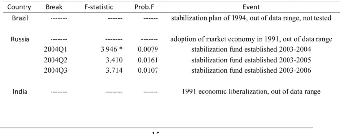
Out of the test results shown in table 4.1 there are breaks only in Russia and South Africa. There is a significant structural change in 2004Q1 for Russia, hence, in the tests afterwards, all data of Russia would be divided into two subgroups: Russia1 (1982Q1-2003Q4) and
Russia2 (2004Q1-2012Q4). For South Africa, the Chow test also confirmed 1994Q1 has
been a significant break. As a result, South Africa is divided into 2 subgroups: S.Africa1
(1982Q1-1993Q4), and S.Africa2 (1994Q1-2012Q4).
Table 4.1 Chow Test
Country Break F-statistic Prob.F Event
Brazil --- --- --- stabilization plan of 1994, out of data range, not tested
Russia --- --- --- adoption of market economy in 1991, out of data range 2004Q1 3.946 * 0.0079 stabilization fund established 2003-2004 2004Q2 3.410 0.0161 stabilization fund established 2003-2005 2004Q3 3.714 0.0107 stabilization fund established 2003-2006
India --- --- --- 1991 economic liberalization, out of data range
16
China --- --- --- Reform and Open-up policies in 1982, as the data begins 2000Q1 1.623 0.1824 1999-2000 tighten monetary policy due to high inflation 2000Q2 1.843 0.1345 1999-2000 tighten monetary policy due to high inflation 2000Q3 1.566 0.1973 1999-2000 tighten monetary policy due to high inflation 2000Q4 1.585 0.1921 1999-2000 tighten monetary policy due to high inflation 2009Q1 0.704 0.6234 08-09 stimulus plan during global financial crisis 2009Q2 1.105 0.3695 08-09 stimulus plan during global financial crisis 2009Q3 1.117 0.3635 08-09 stimulus plan during global financial crisis 2009Q4 1.399 0.2409 08-09 stimulus plan during global financial crisis
S.Africa 1994Q1 8.301 * 0.0000 1993-1994 encouragement of market economy
Note: i.)* Star indicates significance at 1% level (null hypothesis of no breaks rejected: there is significant break). ii).Event column explained briefly the motivation of suspected breakpoint choose, and is detailed in following text.
4.2
Unit Root Test
In macroeconomics data, non-stationary (i.e. there is some general trend) could often be another feature observed. For example, GDP of a certain country would understandably has an increasing trend throughout time. To test such non-stationary, unit root test using Phillips-Perron method can be performed (Phillips, 1998; also known as PP test, non-parametric).
According to Lütkepohl and Krätzig (2004), a PP test with an intercept and time trend builds on the OLS estimation of the Dickey-Fuller test, specifically: , where ∆ is the first difference operator,
a
0 is the intercept,a
1t
is the time trend term, andu
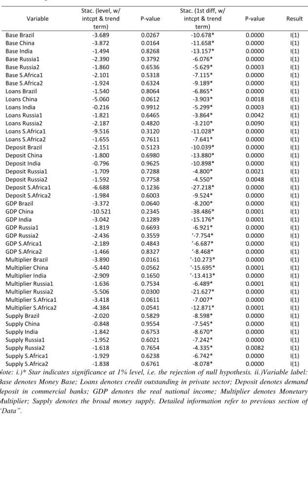
t is an error term. The null hypothesis is that there is a unit root, that is, δ = 0. The test on hypothesis of stationary continues to which the order of integration produces a stationary result. The order of integration, denoted I(d), as defined as the “minimum number of differences required to obtain a covariance stationary series” (Lütkepohl and Krätzig, 2004). Firstly, unit root test conducted on level, if the null hypothesis of there is one unit root cannot be rejected, that means the series is non-stationary; and then test continues in first difference.The results of Unit Root Test are shown in table 4.2. In fact, the findings are that all variables are non-stationary, which makes economic sense. As in macroeconomics, most of the time series data has a general trend. Figure 4.1 plots the variables against time to give a more intuitive view on the increasing trend most variables have.
17 Table 4.2 Phillips-Perron Test
Variable
Stac. (level, w/ intcpt & trend
term)
P-value
Stac. (1st diff, w/ intcpt & trend
term)
P-value Result Base Brazil -3.689 0.0267 -10.678* 0.0000 I(1) Base China -3.872 0.0164 -11.658* 0.0000 I(1) Base India -1.494 0.8268 -13.157* 0.0000 I(1) Base Russia1 -2.390 0.3792 -6.076* 0.0000 I(1) Base Russia2 -1.860 0.6536 -5.629* 0.0003 I(1) Base S.Africa1 -2.101 0.5318 -7.115* 0.0000 I(1) Base S.Africa2 -1.924 0.6324 -9.189* 0.0000 I(1) Loans Brazil -1.540 0.8064 -6.865* 0.0000 I(1) Loans China -5.060 0.0612 -3.903* 0.0018 I(1) Loans India -0.216 0.9912 -5.299* 0.0003 I(1) Loans Russia1 -1.821 0.6465 -3.864* 0.0042 I(1) Loans Russia2 -2.187 0.4820 -3.210* 0.0090 I(1) Loans S.Africa1 -9.516 0.3120 -11.028* 0.0000 I(1) Loans S.Africa2 -1.655 0.7611 -7.641* 0.0000 I(1) Deposit Brazil -2.151 0.5123 -10.039* 0.0000 I(1) Deposit China -1.800 0.6980 -13.880* 0.0000 I(1) Deposit India -0.796 0.9625 -10.898* 0.0000 I(1) Deposit Russia1 -1.709 0.7288 -4.800* 0.0021 I(1) Deposit Russia2 -1.592 0.7758 -4.550* 0.0048 I(1) Deposit S.Africa1 -6.688 0.1236 -27.218* 0.0000 I(1) Deposit S.Africa2 -1.984 0.6003 -9.524* 0.0000 I(1) GDP Brazil -3.372 0.0640 -8.200* 0.0000 I(1) GDP China -10.521 0.2345 -38.486* 0.0001 I(1) GDP India -3.042 0.1289 -15.176* 0.0001 I(1) GDP Russia1 -1.819 0.6693 -6.921* 0.0000 I(1) GDP Russia2 -2.436 0.3559 ‘-7.754* 0.0000 I(1) GDP S.Africa1 -2.189 0.4843 ’-6.687* 0.0000 I(1) GDP S.Africa2 -1.466 0.8327 ‘-8.468* 0.0000 I(1) Multiplier Brazil -3.890 0.0161 ’-10.273* 0.0000 I(1) Multiplier China -5.440 0.0562 ‘-15.695* 0.0001 I(1) Multiplier India -2.909 0.1650 ’-13.413* 0.0000 I(1) Multiplier Russia1 -1.636 0.7534 -6.489* 0.0001 I(1) Multiplier Russia2 -5.506 0.0300 -21.627* 0.0000 I(1) Multiplier S.Africa1 -3.418 0.0611 -7.007* 0.0000 I(1) Multiplier S.Africa2 -4.384 0.0541 -12.871* 0.0001 I(1) Supply Brazil -2.020 0.5829 -8.598* 0.0000 I(1) Supply China -0.848 0.9554 -7.545* 0.0000 I(1) Supply India -1.842 0.6753 -8.670* 0.0000 I(1) Supply Russia1 -1.952 0.6021 -7.242* 0.0000 I(1) Supply Russia2 -1.618 0.7654 -4.335* 0.0082 I(1) Supply S.Africa1 -1.929 0.6238 -6.742* 0.0000 I(1) Supply S.Africa2 -1.838 0.6761 -8.078* 0.0000 I(1)
Note: i.)* Star indicates significance at 1% level, i.e. the rejection of null hypothesis. ii.)Variable label: Base denotes Money Base; Loans denotes credit outstanding in private sector; Deposit denotes demand deposit in commercial banks; GDP denotes the real national income; Multiplier denotes Monetary Multiplier; Supply denotes the broad money supply. Detailed information refer to previous section of “Data”.
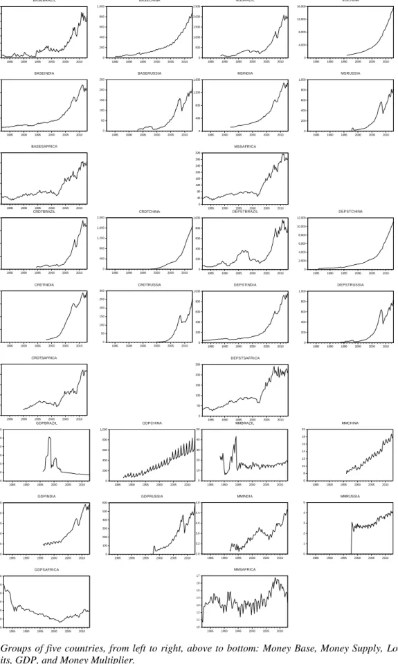
18 Figure 4.1 Trend of Variables
Note: Groups of five countries, from left to right, above to bottom: Money Base, Money Supply, Loans, Deposits, GDP, and Money Multiplier.
0 20 40 60 80 100 120 140 1985 1990 1995 2000 2005 2010 BASEBRAZIL 0 200 400 600 800 1,000 1985 1990 1995 2000 2005 2010 BASECHINA 0 100 200 300 400 1985 1990 1995 2000 2005 2010 BASEINDIA 0 50 100 150 200 250 1985 1990 1995 2000 2005 2010 BASERUSSIA 0 5 10 15 20 25 1985 1990 1995 2000 2005 2010 BASESAFRICA 0 500 1,000 1,500 2,000 2,500 1985 1990 1995 2000 2005 2010 MSBRAZIL 0 4,000 8,000 12,000 16,000 1985 1990 1995 2000 2005 2010 MSCHINA 0 400 800 1,200 1,600 1985 1990 1995 2000 2005 2010 MSINDIA 0 200 400 600 800 1,000 1985 1990 1995 2000 2005 2010 MSRUSSIA 0 40 80 120 160 200 240 280 320 1985 1990 1995 2000 2005 2010 MSSAFRICA 0 100 200 300 400 1985 1990 1995 2000 2005 2010 CRDTBRAZIL 0 400 800 1,200 1,600 2,000 1985 1990 1995 2000 2005 2010 CRDTCHINA 0 40 80 120 160 1985 1990 1995 2000 2005 2010 CRDTINDIA 0 50 100 150 200 250 300 1985 1990 1995 2000 2005 2010 CRDTRUSSIA .00 .05 .10 .15 .20 .25 1985 1990 1995 2000 2005 2010 CRDTSAFRICA 0 200 400 600 800 1,000 1985 1990 1995 2000 2005 2010 DEPSTBRAZIL 0 2,000 4,000 6,000 8,000 10,000 12,000 1985 1990 1995 2000 2005 2010 DEPSTCHINA 0 200 400 600 800 1,000 1985 1990 1995 2000 2005 2010 DEPSTINDIA 0 200 400 600 800 1,000 1985 1990 1995 2000 2005 2010 DEPSTRUSSIA 0 50 100 150 200 250 1985 1990 1995 2000 2005 2010 DEPSTSAFRICA 0 10 20 30 40 50 60 1985 1990 1995 2000 2005 2010 GDPBRAZIL 0 200 400 600 800 1,000 1985 1990 1995 2000 2005 2010 GDPCHINA 0 100 200 300 400 500 1985 1990 1995 2000 2005 2010 GDPINDIA 0 100 200 300 400 500 600 1985 1990 1995 2000 2005 2010 GDPRUSSIA 0 200 400 600 800 1,000 1,200 1985 1990 1995 2000 2005 2010 GDPSAFRICA 0 10 20 30 40 50 1985 1990 1995 2000 2005 2010 MMBRAZIL 6 8 10 12 14 16 18 20 1985 1990 1995 2000 2005 2010 MMCHINA 2.8 3.2 3.6 4.0 4.4 4.8 1985 1990 1995 2000 2005 2010 MMINDIA 0 1 2 3 4 5 1985 1990 1995 2000 2005 2010 MMRUSSIA 10 11 12 13 14 15 16 17 1985 1990 1995 2000 2005 2010 MMSAFRICA
19
4.3
Johansen Cointegration Test
After the stationary test, cointegration test can be proceed, pairwise Johansen test (1988) used to test if there is any long run relationship between two variables.
4.3.1 Lag Determination
As researchers point out, for example Emerson (2007), the Johansen test is highly influenced by the lag lengths. Because of this lag sensitivity, the optimum lag length should be obtained from VAR estimation on variables for each country. The general form of VAR estimation is as the equation 4.1.
Equation 4.1 Vector Autoregressions (VAR) Model
This is a general VAR model with lag of p, A1 ,… ,Ap, B are the matrices of coefficients,
and
e
tis vector of innovations (Emerson, 2007). For quarterly data, a maximum of 5 tested is sufficient.
The Schwarz Criterion choose the lag length j to minimize the value of: log(SSR(j)/n) + (j + 1)log(n)/n, where SSR(j) is the sum or squared residuals for the VAR with j lags and n is the number of observations. (Schwarz 1978).
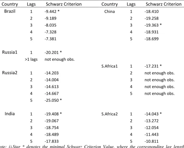
The optimum lag is the one minimizes the Schwarz Criterion Value (Schwarz 1978). The number with a star in table 4.3 is the minimal Schwarz Criterion Value and its corresponding lag length.
20
Table 4.3 Optimal Lag Length for Johansen Cointegration Test
Country Lags Schwarz Criterion Country Lags Schwarz Criterion
Brazil 1 -9.442 * China 1 -18.410 2 -9.189 2 -19.258 3 -8.035 3 -19.363 * 4 -7.328 4 -18.931 5 -7.381 5 -18.699 Russia1 1 -20.201 * >1 lags not enough obs.
S.Africa1 1 -17.231 *
Russia2 1 -14.203 2 not enough obs.
2 -14.004 3 not enough obs.
3 -14.613 4 not enough obs.
4 -14.667 5 not enough obs.
5 -25.050 * India 1 -19.408 * S.Africa2 1 -14.043 * 2 -19.067 2 -13.272 3 -18.754 3 -12.054 4 -18.489 4 -11.443 5 -17.833 5 -10.811
Note: i).Star * denotes the minimal Schwarz Criterion Value, where the corresponding lag length is optimal. ii).Time period: Russia1(1982Q1-2003Q4), Russia2(2004Q1-2012Q4), S.Africa1(1982Q1-1993Q4), S.Africa2(1994Q1-2012Q4).
From table above, the optimum lag lengths for each country: Brazil: 1; Russia1: 1; Russia2: 5; India: 1; China: 3; S.Africa1: 1; S.Africa2: 1. Next, the optimum lag length would be used in the Johansen cointegration test and other tests to come.
4.3.2 Cointegration Test
If the series in inspection share a common stochastic drift, then they are cointegrated. Cointegration suggests long-run relationship between the series. However, it does not tell the direction of such association (Issler, Engle & Granger 1992). For Johansen cointegration test, Trace statistics and Maximal Eigenvalue statistics are used. The results of this part (cointegration) and of Granger causality Tests (sections 4.4.1, 4.4.2, 4.4.3), are presented in the succeeding section of “Results and Discussion” (section 5, starts on page 24).
21
As the Johansen (1991, 1995) procedure, first of all, VAR model in Equation 4.1, could
be rewritten into: , where, .
If the coefficient matrix π has reduced rank r<n, then there are n * r matrices each with rank r, π=αβ’ that β’yt is stationary. r is the number of cointegrating relationships. The
elements of α are known as the adjustment parameters in the vector error correction model and each column of β is a cointegrating vector. Then the statistics of Trace and Maximal Eigenvalue are: ) ˆ 1 ln( ) 1 , ( ) ˆ 1 ( ) ( 1 1
r Max g r i i Trace T r r in T r ,Where T is sample size,
ˆ
iis the estimated value for the i-th ordered eigenvalue from the π matrix. The trace test tests the null hypothesis of r cointegrating vectors against the alternative hypothesis of n cointegrating vectors. The maximum eigenvalue: null hypothesis of r cointegrating vectors against alternative r+1. (Johansen 1991, 1995; Enders, 2010). In Johansen Cointegration test, if the test statistic > critical value, then the null hypothesis of that there is none (or corresponding numbers of cointegrating equations) should be rejected, otherwise, accept. The result of cointegration test is available in table 5.1.4.4
Causality Tests
4.4.1 Standard Granger Causality Test
Granger non-causality (or causality) test is applied to study causal relationship and causality direction, rather than just correlation between variables. By the instructions of Toda & Yamamoto (1995) if the non-stationary series follows I(1) but not cointegrated (as there are many such cases in this paper), then a standard Granger causality test could be applied. As stated by Phillips & Ouliaris (1990), in such cases first difference should be taken for the variables before the application of Granger causality test. Conversely, if two variables are cointegrated, as Granger (1988) explained, VECM (Vector Error Correction Model) method of the Granger causality test should be practiced.
Consider a general case with pairs of (x,y) series and optimal lag length of l (Gujarati 2009), Granger causality test runs bivariate regressions on:
22 Equation 4.2 Granger Causality Test
The null hypothesis is that, for each equation all the
β
s jointly equals to 0, i.e. independent variable does not Granger cause the dependent variable. Granger causality test results are obtainable in table 5.2 (page 27).4.4.2 VECM
The VECM method are explained by Granger & Weiss (1983) and Granger (1969, 1988)9.
VECM is used in the “first-difference stationary” situations. It can be used to test the short-run and long-short-run causality between a dependent variable and an independent variable: the long-run causality (from independent variable to dependent variable) can be identified in the test of the significance of the error-correction coefficient of the VECM by using ordinary least squares (OLS) estimation of the model. Wald test, on the other hand, tests the significance of coefficients of independent variables, to determine short-run causality. Together with Granger causality test, the results (in section 5 page 27) can answer the first three research questions regarding the causality direction (see section 1.1).
Equation 4.3 Vector Error Correction
As Pesaran (1995) explained, the general Vector Error Correction Model is as equation 4.3. Using the same model as VAR of equation 4.2, but with an additional Error Correction Term ( ). Similar to the Granger causality Test, short-term causality of the VECM follows Wald test (Chi-square, to test if the coefficients jointly equals to 0). Long-term causality could be tested to see if the error-correction coefficient
α
3is significant. Result of VECM tests are detailed in section 5, summarized in table 5.3 (page 29).
23
4.4.3 Trivariate VAR
To further examine the causality directions of the variables and to answer the research question 4 (page 5) of this study, a trivariate (namely loans, deposit and money supply) VAR model is used. Furthermore, by including the variable deposit, which did not occur in previous research questions, could test the validity of previous Granger causality in control of deposit variable. This would also provide information on which influence channel of money supply the country’s empirical data would be fit.
Similar to bivariate VECM, significance of the Error Correction Term expresses the long-run causality of the trivariate model, meanwhile joint significance of coefficients of corresponding of independent variables tells the short-run causality. The direction is from independent variable to dependent variable
Based on Toda and Yamamoto (1995), Pesaran (1995) and Badarudin et al. (2013), similar to the previous VAR models, a trivariate VAR (k, dmax) model matrix can take the form of
such:
Equation 4.4 Trivariate VAR Matrix
Where, k and dmax are the lag length and maximum order of integration respectively; βi ,βj
are the 3*3 matrices represent the coefficients. To test if there is causality from bank loans to deposits: the null hypothesis is no causality, , where are coefficients consistent with k –th lag of the variable
𝑦
1,𝑡−𝑖 in equation 4.4. Similarity, during the tests, the three variables this paper intends to investigate take the dependent variabley
1in turns. The test statistics are also similar to the VECM ones in previous section. The results are also in the coming section, see table 5.5.24
5
Results and Discussion
5.1
Results in Previous Section
The results of relatively simple tests were presented with their test methods in previous section.
Firstly, Phillips-Perron Unit Root Tests implemented and indications that all variables for the BRICS countries are non-stationary, detailed results see table 4.2.
Secondly, by the Schwarz Bayesian Information Criteria, the optimal lag length for the cointegration tests and VECM tests has been found. Specifically, one can refer to table 4.3: Russia 2: 5 lags; China, 3 lags; other countries have the optimum lag length of 1.
5.2
Cointegration Results
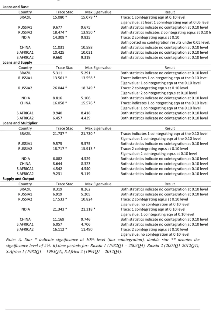
After the determination of optimal lag lengths, Johansen Cointegration Test could be continues. To test if the variables has long-run correlation between each other, pairwise cointegration tests have been performed: bank loans and monetary base; banks loans and money supply; bank loans and monetary multiplier; and lastly money supply and the output. Cointegration indicates that association existing in the two series but cannot show us the direction, and the results are summarized into the following table 5.1.
25 Table 5.1 Johansen Cointegration Test
a) Loans and Base
Country Trace Stac Max.Eigenvalue Result BRAZIL 15.080 * 15.079 ** Trace: 1 cointegrating eqn at 0.10 level
Eigenvalue: at least 1 conintegrating eqn at 0.05 level RUSSIA1 9.677 9.675 Both statistics indicate no cointegration at 0.10 level RUSSIA2 18.474 * 13.950 * Both statistics indicates 2 cointegrating eqn.s at 0.10 level
INDIA 14.308 * 9.825 Trace: 2 cointegrating eqn.s at 0.10
Both posted no cointegration results under 0.05 level. CHINA 11.031 10.588 Both statistics indicate no cointegration at 0.10 level S.AFRICA1 10.425 10.031 Both statistics indicate no cointegration at 0.10 level S.AFRICA2 9.660 9.319 Both statistics indicate no cointegration at 0.10 level
b) Loans and Supply
Country Trace Stac Max.Eigenvalue Result
BRAZIL 5.311 5.291 Both statistics indicate no cointegration at 0.10 level RUSSIA1 13.561 * 13.558 * Trace: indicates 1 cointegrating eqn at the 0.10 level
Eigenvalue: 1 cointegrating eqn at the 0.10 level RUSSIA2 26.044 * 18.349 * Trace: 2 cointegrating eqn.s at 0.10 level
Eigenvalue: 2 cointegrating eqn.s at 0.10 level INDIA 8.816 5.106 Both statistics indicate no cointegration at 0.10 level CHINA 16.058 * 15.576 * Trace: indicates 1 cointegrating eqn at the 0.10 level
Eigenvalue: 1 cointegrating eqn at the 0.10 level S.AFRICA1 9.940 8.418 Both statistics indicate no cointegration at 0.10 level S.AFRICA2 6.457 4.439 Both statistics indicate no cointegration at 0.10 level
c) Loans and Multiplier
Country Trace Stac Max.Eigenvalue Result
BRAZIL 21.737 * 21.730 * Trace: indicates 1 cointegrating eqn at the 0.10 level Eigenvalue: 1 cointegrating eqn at the 0.10 level RUSSIA1 9.575 9.575 Both statistics indicate no cointegration at 0.10 level RUSSIA2 18.717 * 15.913 * Trace: 2 cointegrating eqn.s at 0.10 level
Eigenvalue: 2 cointegrating eqn.s at 0.10 level INDIA 6.082 4.529 Both statistics indicate no cointegration at 0.10 level CHINA 8.644 8.323 Both statistics indicate no cointegration at 0.10 level S.AFRICA1 4.542 4.540 Both statistics indicate no cointegration at 0.10 level S.AFRICA2 9.231 9.119 Both statistics indicate no cointegration at 0.10 level
d) Supply and Output
Country Trace Stac Max.Eigenvalue Result
BRAZIL 8.319 8.262 Both statistics indicate no cointegration at 0.10 level RUSSIA1 6.919 5.205 Both statistics indicate no cointegration at 0.10 level RUSSIA2 17.533 * 10.824 Trace: 2 cointegrating eqn.s at 0.10 level
Eigenvalue: no cointegration at 0.10 level INDIA 21.343 * 21.318 * Trace: 1 cointegrating eqn at 0.10 level
Eigenvalue: 1 cointegrating eqn at 0.10 level CHINA 11.169 9.746 Both statistics indicate no cointegration at 0.10 level S.AFRICA1 6.057 4.706 Both statistics indicate no cointegration at 0.10 level S.AFRICA2 16.112 * 11.490 Trace: 2 cointegrating eqn.s at 0.10 level
Eigenvalue: no cointegration at 0.10 level
Note: i). Star * indicate significance at 10% level (has cointegration), double star ** denotes the significance level of 5%. ii).time periods for: Russia 1 (1982Q1 – 2003Q4), Russia 2 (2004Q1-2012Q4); S.Africa 1 (1982Q1 – 1993Q4), S.Africa 2 (1994Q1 – 2012Q4).
26
As the table 5.1 revealed, almost half of the null hypothesis of no cointegration relationships found to be accepted. For example, for the three countries of Brazil, India, South Africa, Banks loans and money supply are not in long-run relationships; only Russia2, India, South Africa 2 found the relationship in income and money supply.
The results in the table suggested more tests needed to be done to draw any concluding interpretations. The cointegration test only shown few findings on long-run relations without indicating causality or direction. As the next step, Granger causality tests applied to no-cointegrated variables and VECM tests for no-cointegrated ones.
5.3
Causality Test Results
After the determination of long-term relationships by cointegration, they are further examined by using Granger causality tests. As in section “Econometrics Method” explained, if variables are not cointegrated, can be proceed with standard Version of Granger causality test.
Conversely, if two variables are cointegrated, a VECM version of Granger causality should be applied (equation 4.3).
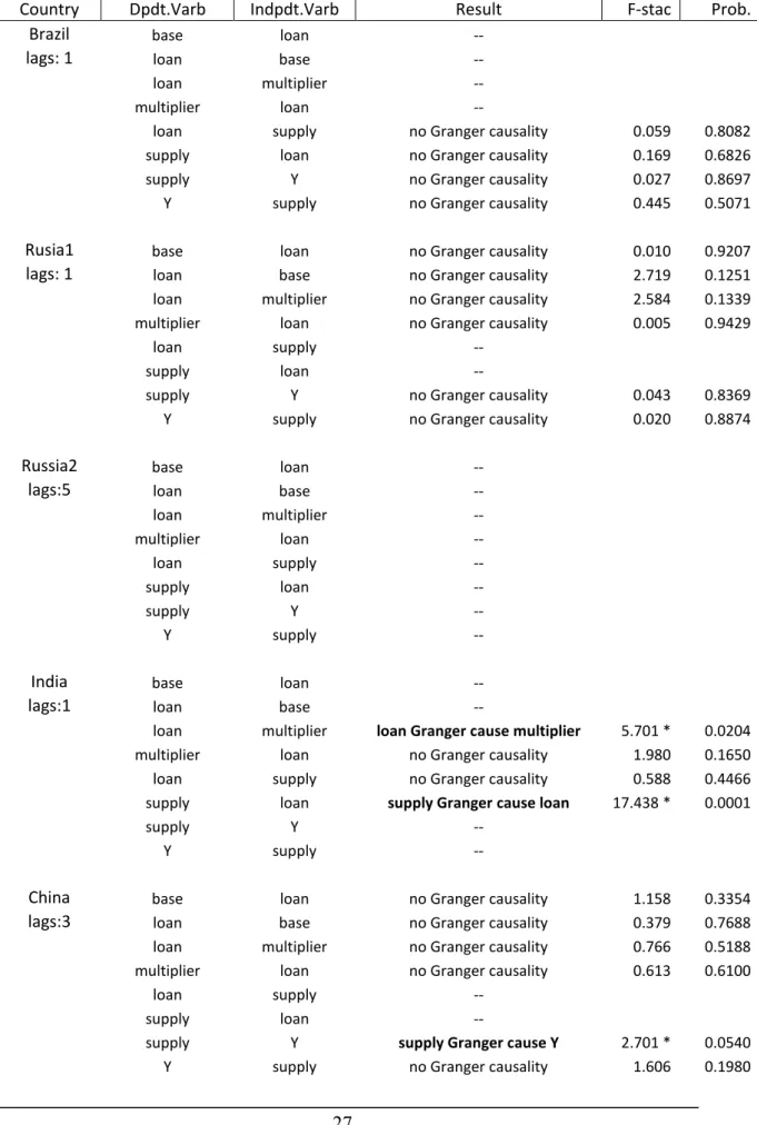
The Granger causality test results for no-cointegration variables are potted in the next table.
27 Table 5.2 Granger Causality test
Country Dpdt.Varb Indpdt.Varb Result F-stac Prob.
Brazil base loan --
lags: 1 loan base --
loan multiplier --
multiplier loan --
loan supply no Granger causality 0.059 0.8082
supply loan no Granger causality 0.169 0.6826
supply Y no Granger causality 0.027 0.8697
Y supply no Granger causality 0.445 0.5071
Rusia1 base loan no Granger causality 0.010 0.9207
lags: 1 loan base no Granger causality 2.719 0.1251
loan multiplier no Granger causality 2.584 0.1339
multiplier loan no Granger causality 0.005 0.9429
loan supply --
supply loan --
supply Y no Granger causality 0.043 0.8369
Y supply no Granger causality 0.020 0.8874
Russia2 base loan --
lags:5 loan base --
loan multiplier -- multiplier loan -- loan supply -- supply loan -- supply Y -- Y supply --
India base loan --
lags:1 loan base --
loan multiplier loan Granger cause multiplier 5.701 * 0.0204
multiplier loan no Granger causality 1.980 0.1650
loan supply no Granger causality 0.588 0.4466
supply loan supply Granger cause loan 17.438 * 0.0001
supply Y --
Y supply --
China base loan no Granger causality 1.158 0.3354
lags:3 loan base no Granger causality 0.379 0.7688
loan multiplier no Granger causality 0.766 0.5188
multiplier loan no Granger causality 0.613 0.6100
loan supply --
supply loan --
supply Y supply Granger cause Y 2.701 * 0.0540
28
S.Africa1 base loan base Granger cause loan 6.938 * 0.0218
lags:1 loan base loan Granger cause base 3.218 * 0.0980
loan multiplier no Granger causality 3.043 0.1066 multiplier loan multiplier Granger cause loan 8.516 * 0.0129
loan supply no Granger causality 0.002 0.9694
supply loan no Granger causality 0.323 0.5802
supply Y no Granger causality 0.062 0.8041
Y supply Y Granger cause supply 3.252 * 0.0782
S.Africa2 base loan no Granger causality 0.017 0.8969
lags:1 loan base loan Granger cause base 2.824 * 0.0972
loan multiplier no Granger causality 0.406 0.5259
multiplier loan no Granger causality 0.060 0.8077
loan supply no Granger causality 0.010 0.9210
supply loan no Granger causality 0.011 0.9180
supply Y --
Y supply --
Note: i) Granger Causality tests are conducted at 10% level of significance (if non-cointegration, first difference taken), Star *, denotes causality, direction is from independent variable to dependent variable. ii).Time Periods: Russia 1 (1982Q1 – 2003Q4), Russia 2 (2004Q1-2012Q4); S.Africa 1 (1982Q1 – 1993Q4), S.Africa 2 (1994Q1 – 2012Q4). iii). variable label: ‘Base’ denotes Money Base; ‘loan’ denotes Bank Loans, i.e. Credits Outstanding; ‘Y’ denotes the Real Output; ‘Multiplier’ denotes Monetary Multiplier; ‘Supply’ denotes Broad Money Supply.
Still, out of various tests conducted, only in eight cases, there is Granger causality found. Thus, conclusion may be drawn only after the combination of all the causality tests results this thesis intended to conduct.
29
5.3.1 VECM Results
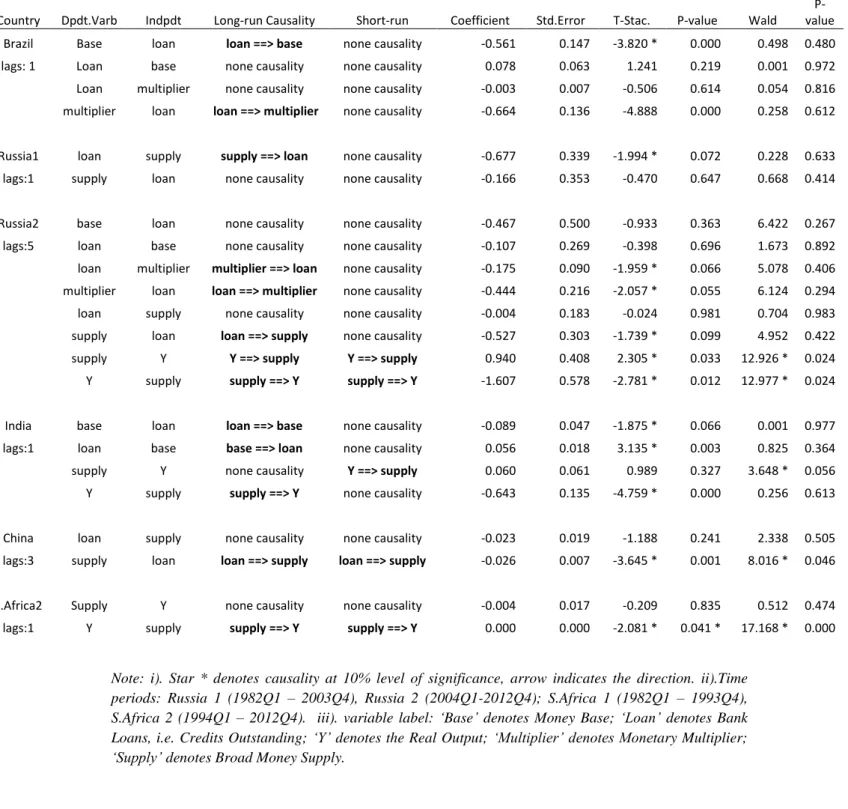
By means explained in the Econometrics Method section, the significance of error correction term and joint significance of coefficients can reflect the long-term and short-term causality. Results are available in table 5.3, as follows. Then in the succeeding table 5.4, a combined causality results from previous sections provided insights on the bank loan and money supply relationships of the ‘BRICS’ group.
Table 5.3 Vector Error Correction Model
Country Dpdt.Varb Indpdt Long-run Causality Short-run Coefficient Std.Error T-Stac. P-value Wald P-value Brazil Base loan loan ==> base none causality -0.561 0.147 -3.820 * 0.000 0.498 0.480 lags: 1 Loan base none causality none causality 0.078 0.063 1.241 0.219 0.001 0.972 Loan multiplier none causality none causality -0.003 0.007 -0.506 0.614 0.054 0.816 multiplier loan loan ==> multiplier none causality -0.664 0.136 -4.888 0.000 0.258 0.612 Russia1 loan supply supply ==> loan none causality -0.677 0.339 -1.994 * 0.072 0.228 0.633 lags:1 supply loan none causality none causality -0.166 0.353 -0.470 0.647 0.668 0.414 Russia2 base loan none causality none causality -0.467 0.500 -0.933 0.363 6.422 0.267 lags:5 loan base none causality none causality -0.107 0.269 -0.398 0.696 1.673 0.892 loan multiplier multiplier ==> loan none causality -0.175 0.090 -1.959 * 0.066 5.078 0.406 multiplier loan loan ==> multiplier none causality -0.444 0.216 -2.057 * 0.055 6.124 0.294 loan supply none causality none causality -0.004 0.183 -0.024 0.981 0.704 0.983 supply loan loan ==> supply none causality -0.527 0.303 -1.739 * 0.099 4.952 0.422 supply Y Y ==> supply Y ==> supply 0.940 0.408 2.305 * 0.033 12.926 * 0.024 Y supply supply ==> Y supply ==> Y -1.607 0.578 -2.781 * 0.012 12.977 * 0.024 India base loan loan ==> base none causality -0.089 0.047 -1.875 * 0.066 0.001 0.977 lags:1 loan base base ==> loan none causality 0.056 0.018 3.135 * 0.003 0.825 0.364 supply Y none causality Y ==> supply 0.060 0.061 0.989 0.327 3.648 * 0.056 Y supply supply ==> Y none causality -0.643 0.135 -4.759 * 0.000 0.256 0.613 China loan supply none causality none causality -0.023 0.019 -1.188 0.241 2.338 0.505 lags:3 supply loan loan ==> supply loan ==> supply -0.026 0.007 -3.645 * 0.001 8.016 * 0.046 S.Africa2 Supply Y none causality none causality -0.004 0.017 -0.209 0.835 0.512 0.474 lags:1 Y supply supply ==> Y supply ==> Y 0.000 0.000 -2.081 * 0.041 * 17.168 * 0.000
Note: i). Star * denotes causality at 10% level of significance, arrow indicates the direction. ii).Time periods: Russia 1 (1982Q1 – 2003Q4), Russia 2 (2004Q1-2012Q4); S.Africa 1 (1982Q1 – 1993Q4), S.Africa 2 (1994Q1 – 2012Q4). iii). variable label: ‘Base’ denotes Money Base; ‘Loan’ denotes Bank Loans, i.e. Credits Outstanding; ‘Y’ denotes the Real Output; ‘Multiplier’ denotes Monetary Multiplier; ‘Supply’ denotes Broad Money Supply.
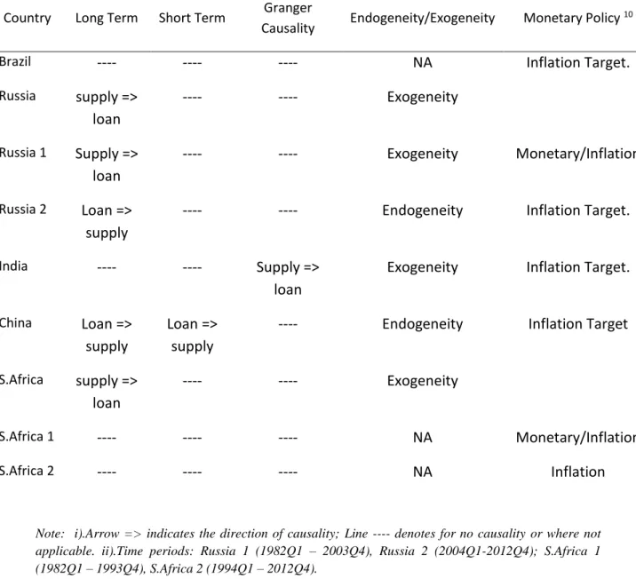
30 Table 5.4 Relationship b/t Money Supply and Loans
Country Long Term Short Term Granger
Causality Endogeneity/Exogeneity Monetary Policy
10
Brazil ---- ---- ---- NA Inflation Target.
Russia supply => loan ---- ---- Exogeneity Russia 1 Supply => loan ---- ---- Exogeneity Monetary/Inflation Russia 2 Loan => supply
---- ---- Endogeneity Inflation Target.
India ---- ---- Supply =>
loan
Exogeneity Inflation Target.
China Loan => supply
Loan => supply
---- Endogeneity Inflation Target
S.Africa supply => loan
---- ---- Exogeneity
S.Africa 1 ---- ---- ---- NA Monetary/Inflation
S.Africa 2 ---- ---- ---- NA Inflation
Note: i).Arrow => indicates the direction of causality; Line ---- denotes for no causality or where not applicable. ii).Time periods: Russia 1 (1982Q1 – 2003Q4), Russia 2 (2004Q1-2012Q4); S.Africa 1 (1982Q1 – 1993Q4), S.Africa 2 (1994Q1 – 2012Q4).
As expected, during the contemporary age inflation targeting became the main objective for the central banks across the five economies. However, only China and Russia (2004-2012) shows signs of money supply endogeneity, which is in line with Badarudin (2009), and Vymyatnina (2006). The results should be confirmed and improved by later test of trivariate VAR that includes deposit.
31
The exogeneity shared by other three countries may be contributed to the reason that: First, Economic growth and development has not yet stabilized which in turn causing disturbance in money demand and effecting money supply from the demand side. Secondly, during the economic boost, and at the same time government put the stabilization of price level above all, hence, if other ways cannot be done or proven ineffective, the monetary authority has to take tight control over the money stock.
This explanation shared by various developing or undeveloped countries which evidently sharing the same growing inflation problem11. Meanwhile China and the recent period of
Russia Federation, has already experienced the “growing pain”. They, in modern time, has relatively less control and mature policy decisions concerning money aggregates. Moreover, they have gradually relaxed monetary targeting, allowing for some room of inflation in order to keep the GDP growth going upward.
5.4
Trivariate VAR Results
To further confirm the robust or reject (if found invalid) the findings above, and to investigate whether bank deposit is important in the causality link (the transmission channel), a Trivariate VECM model used (money supply, bank loans and deposits. See section “Econometrics Method”).
Results of trivariate tests are available in the following page, table 5.5.
11 Luintel (2002) for South Asia countries, Badarudin (2009) for Mexico, Indonesia, Russia, Taiwan.
Ghartey (1998) Jamaica, Chigbu (2013) for Nigeria. For historical, see Beyer (1998) study on 1975-1994’s Germany under-going the unification.
32 Table 5.5 Trivariate VAR
Country Depdt Varb Indepdts Results Lomg-Term
Brazil loan deposit supply both insignificant insignificant deposit loan supply both insignificant insignificant supply loan deposit deposit ==> supply insignificant
Russia loan deposit supply deposit ==> loans deposit&supply => loan deposit loan supply both insignificant loan&supply => deposit supply loan deposit both insignificant loan&deposit => supply
Russia1 loan deposit supply both insignificant insignificant (82’-03’) deposit loan supply both insignificant insignificant supply loan deposit deposit ==> supply insignificant
Russia2 loan deposit supply deposit, supply ==> loan insignificant (04’-12’) deposit loan supply both insignificant loan&supply => deposit
supply loan deposit deposit ==> supply loan&deposit => supply
India loan deposit supply supply => loan insignificant deposit loan supply both insignificant loan&supply => deposit supply loan deposit both insignificant insignificant
China loan deposit supply both insignificant insignificant deposit loan supply both insignificant loan&supply => deposit supply loan deposit loan,deposit ==> supply loan&deposit => supply
S.Africa loan deposit supply both insignificant deposit&supply=> loan deposit loan supply both insignificant loan&supply => deposit supply loan deposit both insignificant insignificant
S.Africa1 loan deposit supply both insignificant insignificant (82’-93’) deposit loan supply both insignificant insignificant
supply loan deposit both insignificant loan&deposit => supply
S.Africa2 loan deposit supply both insignificant deposit&supply => loan (94’-12’) deposit loan supply both insignificant loan&supply => deposit supply loan deposit both insignificant loan&deposit => supply
Note: i). At level 10%, arrow => indicates the direction ii).Time periods: Russia 1 (1982Q1 – 2003Q4), Russia 2 (2004Q1-2012Q4); S.Africa 1 (1982Q1 – 1993Q4), S.Africa 2 (1994Q1 – 2012Q4). iii). variable labels:
‘Loan’ denotes Bank Loans, ie. Credits Outstanding; ‘deposit’ denotes Bank Deposits; ’supply’: Money Supply.