Centralization of inventory management for spare parts

(1)

Centralization of inventory management for spare parts

-

A case study on its performance compared to the current inventory

control system at Arriva DK Master’s thesis project

Stefan Petersson, Simon Sturesson

Supervisor at Lund University, Faculty of Engineering: Sven Axsäter Supervisor at Arriva DK: Stefan Vidgren

Division of Production Management

Lund University

(2)

I

Preface

This master’s thesis is the final part of the Master of Science programs Mechanical Engineering, and Industrial Engineering and Management at Lund University, Faculty of Engineering. The thesis corresponds to 30 ECT points and was conducted during the summer and fall of 2013 on initiatives from Arriva DK.

We would like to thank our supervisor Sven Axsäter at Lund University and Stefan Vidgren, Arriva DK for making this thesis possible.

We would like to thank Sven Axsäter for his help with our thesis. We would also like to thank Stefan for all his support and feedback he has given us during the thesis. We would also like to thank Lars Bonke at Arriva DK for his support and help during our study visit. Finally, we would like to thank everyone we met during our visits to Arriva.

Lund, January 2014

Stefan Petersson Simon Sturesson

(3)

II

Abstract

Title

Centralization of inventory management for spare parts - A case study on its performance compared to the current inventory control system at Arriva DK Authors

Stefan Petersson and Simon Sturesson Supervisors

Sven Axsäter, Faculty of Engineering, LTH Stefan Vidgren, Arriva DK

Background

Arriva DK currently has a decentralized organization where each depot is responsible for the inventory control of their spare parts. This type of organization often presents challenges when it comes to control and management. Arriva DK suffers from high order costs due to lack of coordination between the depots and the suppliers. To address these issues Arriva wants to introduce a central warehouse.

Purpose

The aim of the thesis is to optimize inventory management by creating simulation models that from a cost perspective explore the effects of introducing a central warehouse for spare parts.

To provide Arriva DK with simulation models of the supply chain and inventory management, both with – and without a central warehouse.

Method

The thesis is built on Hillier and Lieberman’s Operations research method. Data used in the thesis consist of both primary and secondary quantitative and qualitative data. Literature studies have also been done and are the basis for the theory. Two simulation models were built. The first model represents an optimized decentralized situation that uses joint replenishment. The second model represents a system with a central warehouse, which also uses joint replenishment. Thereafter the models were compared to determine if an investment in a centralized system is profitable.

(4)

III Conclusions

The results from the simulation study showed that the total cost for the CW-model is higher than the DC-CW-model in all scenarios. Both the holding- and order cost will be higher with a central warehouse.

The major advantage of using a central warehouse is that the number of orders to the suppliers will be reduced by more than 50%. This along with the suppliers only have to deliver to one location will result in price reductions on the products. Even with small discounts, will a central warehouse be profitable since the procurement cost represents such a large part of the total cost.

(5)

IV

1. Introduction

In this chapter the background, purpose, delimitations, problem formulation and target group are discussed. This chapter will also provide a brief company description of Arriva Dk. Finally a report outline is discussed.

1.1 Background

Supply Chain Management, the control of the flow of goods, is recognised as a central activity in most enterprises. Inventory control is a very important component in a supply chain. Investments in inventories are enormous which means that the inventory levels should be kept at a minimum. High inventory levels, however, avoids shortages and large order costs. Finding a balance between these goals offers an important potential for improvement.

Arriva DK currently has a decentralized organization where each depot is responsible for the inventory control of their spare parts. This type of organization often presents challenges when it comes to control and management. Arriva DK suffers from high order costs due to lack of coordination between the depots and the suppliers. As a first step, Arriva DK has implemented a joint replenishment policy at the depots. This means that when a depot places an order with a supplier; all products from that supplier are ordered at the same time to reduce the order cost.

Arriva DK feels, however, that there are more room for improvement. With a central warehouse, which functions as a bundling and distribution centre between the suppliers and the depots, even more products can be jointly replenished. The depots can then order a group of products, from the central warehouse; independent of which suppliers they originate from.

At the same time, new costs, such as transportation cost, will arise. The possible benefits and drawbacks, of a central warehouse, will be impossible to scale and quantify without further analysis.

This master thesis focuses on the effects of introducing a central warehouse and centralizing the inventory management. Due to the complexity of the system, simulation will be used as the tool for evaluation. The simulation models and the overall insights, of this project, will then serve as an underlying foundation for similar projects.

(10)

2

1.2 Company Description

Arriva is public transport company and is since 2010 owned by Deutsche Bahn (DB). It was founded in Sunderland, United Kingdom in 1938 and has since the start grown to where it is today with bus, train, waterbus, tram and coach operations in over 12 countries in Europe and currently employs around 55,900 people (Arriva, 2013).

Arriva DK has been part of Denmark’s public transport since 1997 after buying the Danish bus company Unibus. Today, after acquiring several different bus companies, Arriva is Denmark’s largest bus company with a market share of about 50 % and traffics most parts of Denmark with approximately 1300 buses.

The buses are serviced and repaired in different depots across Denmark that also functions as warehouses. A bus only belongs to one depot at a time. All spare parts used are bought from suppliers and delivered to the depots.

1.3 Purpose

The purpose of this project has two parts:

1. The aim of the thesis is to optimize inventory management by creating simulation models that from a cost perspective explore the effects of introducing a central warehouse for spare parts.

2. To provide Arriva DK with simulation models of the supply chain and inventory management, both with – and without a central warehouse.

This project will result in a cost oriented decision support for Arriva DKs management for operating a supply chain with a central warehouse. It will also make it easier to carry out similar projects in other regions or markets thanks to the simulation models created for this project.

1.4 Delimitations

For practical reasons and due to limitations of the simulation software, used in this project, some delimitations have to be made.

(11)

3 Delimitations to the demand:

 The demand for every product is assumed to follow a Poisson process.

 Trends in the demand will not be taken into account.

 The suppliers always deliver complete orders on time. Delimitations to the simulation models:

 The simulation models can handle a maximum of four depots at the same time.

 Each depot can carry up to ten different products.

 The maximum number of suppliers is eight.

 The suppliers can carry up to five different products each.

1.5 Problem Formulation

This project aims to answer two questions:

1. How will Arriva DKs spare parts inventory system perform with a central warehouse compared to without a central warehouse regarding order -, holding - and transportation costs?

2. Under what conditions will a centralized system outperform a decentralized system, from a cost perspective?

1.6 Target Group

The main target group for this master thesis is Arriva DKs management and operations research team. This project has, however, been carried out in a way that it with minor modifications can be applied on other geographical regions with different conditions. This means that the study is also relevant for other companies that are thinking of introducing a central warehouse and wants to use simulation as a tool for analysis. Finally, this thesis can act as an inspiration to students who are interested in inventory control in combination with simulation.

(12)

4

1.7 Report outline

The report is divided into the following sections.

 Chapter 1, Introduction: In this chapter the background, purpose, delimitations, problem formulation and target group are discussed. This chapter will also provide a brief company description of Arriva Dk. Finally a report outline is presented.

 Chapter 2, Methodology: In this chapter the methodology used in the thesis is presented. Initially, the general operations study approach is discussed. Secondly, the approach used in this study is explained and finally, the validity, reliability and objectivity of this study are discussed.

 Chapter 3, Theoretical Framework: The theoretical framework is presented in this chapter. Initially, a brief introduction to inventory control is presented. Then the ordering policy and the costs connected to the models are discussed. Finally, the theory behind a central warehouse and joint replenishment are presented.

 Chapter 4, The Supply Chain Set-Up: This chapter aims to give a background to the real world set-up for the flow of spare parts at Arriva DK and describe the two set-ups used in the simulation study.

 Chapter 5, Simulation scenarios: In this chapter the results from the different simulation scenarios are presented. In order to see if a central warehouse is better than a decentralized model; different scenarios have been created to get different views and outputs.

 Chapter 6, Analysis: In this chapter the analysis of the costs are presented. A trend analysis is also presented as well as an analysis of the organization.

 Chapter 7, Conclusions and discussion: In this chapter the conclusions are presented and discussed.

(13)

5

2. Methodology

In this chapter the methodology used in the thesis is presented. Initially, the general operations study approach is discussed. Secondly, the approach used in this study is explained. Finally, the validity, reliability and objectivity of this study are discussed.

2.1 General Operations Research Study

The approach of this thesis belongs to the field of Operations Research. An operations research study is generally divided into six phases, which usually are overlapping (Hillier & Lieberman, 2005):

1. Define the problem and gather data.

2. Formulate a mathematical model to represent the problem.

3. Develop a computer-based procedure for deriving solutions to the problem from the model.

4. Test the model and refine it as needed.

5. Prepare the ongoing application of the model assigned by management.

6. Implement.

2.1.1 Define the Problem and Gather Data

The first step of an operations research study is to study the relevant system and develop a well-defined statement of the problem. Setting objectives, constraints on what can be done as well as time limits. It is important to involve all partners and make them understand what the problem is (Hillier & Lieberman, 2005). After this step, data is gathered to better understand the problem and to obtain the inputs that are required for the simulation models.

There are two methods to choose from when gathering data. The first one is quantitative data, which is data that can be measured numerically. Mathematical models are generally quantitative. The second one is qualitative data, which is data that aims at providing a comprehensive picture of the situation. Interviews are usually useful for qualitative studies. The collected data can be collected both as primary – and secondary data. Primary data is data that has been collected or created during the projects run. Secondary data is data that already exists and are collected for other purposes than the project.

(14)

6

2.1.2 Represent the Problem by Formulating a Mathematical Model After the problem is defined, the next phase is to reformulate the problem in a form that is convenient for analysis (Hillier & Lieberman, 2005). A mathematical model is constructed and it is important to start with a simple version and then gradually improve it until it represents the problem.

2.1.3 Deriving Solutions From the Model

The third step is to develop a procedure that is usually computer-based that derives solutions to the problem. It is common to search for an optimal solution by applying a standard algorithm or using software to model the problem. However, these solutions are only optimal with respect to the model being used. Since the model is an idealized version there is no guarantee that the solution is an optimal solution for the real problem. If the model is well formulated and tested, the solution should tend to be a good approximation to the problem (Hillier & Lieberman, 2005).

2.1.4 Testing the Model and Refining it as Needed

This step involves testing the model in order to find bugs. Early versions of a model usually contain many bugs that need to be eliminated. This process is commonly referred to as model validation or verification. Verification of the model should be done continuously and not after the entire model is finished. It is important to note that a verified model does not necessarily describe the system accurately. It only means that the model is free from bugs and behaves in the way it should (Hillier & Lieberman, 2005).

2.1.5 Preparing to Apply the Model

The fifth step is to install a well-documented system to prepare for implementing the model as prescribed by management. The system includes the model, solution procedure and operating procedures for implementation (Hillier & Lieberman, 2005).

2.1.6 Implementation

The final step is to implement the solution in the system. For best result it is important that the team that worked with the model is involved with the implementation, since they know the model best. The success of the implementation also depends on the support of top management and operating management (Hillier & Lieberman, 2005).

(15)

7

2.2 The Approach of This Thesis

Hillier and Lieberman’s approach for operations research, described above, is relatively broad and intended to be used to any operations research study. This thesis will not cover step 5 “Prepare the ongoing application of the

model assigned by management” and step 6 “Implement” since they fall

outside the scope of the thesis. This general method will be used as a framework, and modified to fit this thesis.

2.2.1 Define the Problem and Gather Data.

The problem given to the authors was to evaluate the effects of centralizing the inventory management for spare parts by introducing a central warehouse. After discussions with Arriva DK, it was decided to create two models. The first model represents an optimized decentralized situation that uses joint replenishment. The second model represents a system with a central warehouse, which also uses joint replenishment. Thereafter the models will be compared to determine if an investment in a centralized system is profitable.

Interviews at the initial phase of the thesis were held with stock managers at two different warehouses. The interviews with the managers helped to understand the current situation and what the impact of introducing a central warehouse would be. Study visits to the warehouses were also made to get an overall view of the order processing and the inventory management. Furthermore an interview was also made with a supplier to better understand their situation and what problems they have today with the current setup.

After the problem formulation was done the objectives of the study could be set. It was important to get a structure of what was needed and expected from the authors. After discussions with Arriva DK all objectives were set and a project plan with a timeline was made which describes how the work would be conducted.

Data Collection

Data used in the thesis consist of both primary and secondary quantitative and qualitative data. The data gathered from Arriva DK’s ERP-system such as product prices, the total product demand in a year are considered secondary data since it was not created for this project.

Visits to Arriva DK’s warehouses were done in order to interview the stakeholders and collect raw data. Questions were prepared before the

(16)

8

interviews. The costs connected to when an order is made such as handling cost and billing cost were obtained from interviews with Arriva DK’s supply chain manager. This is considered primary data since it was created for this project.

Literature studies have also been done and are the basis for the theory presented in chapter 3. The articles used are from established and respected sources. The books used are from respected authors, which extensive knowledge in the subjects covered. The data obtained is considered secondary since it has been processed and used for other purposes than this thesis.

2.2.2 Analysing Data and Finding a Way to Describe a Product’s Demand Arriva DK carries a vast amount of items and an evaluation of all items through simulation would be impossible. Therefore it was necessary to select a sample of products from different suppliers to represent the inventory system. It was decided that products from eight suppliers were sufficient. The products were selected through ABC analysis, which is a technique to categorize inventory after importance.

An issue we encountered was to describe a product’s demand satisfactory. The only data we could obtain was a product’s total demand in a year. Therefore we have assumed that the customers arrive according to a Poisson process. This is a common assumption in stochastic inventory models (Axsäter, 2006). A Poisson process occurs when arrivals happen one at a time with given intensity, are completely at random and independent of one another. The number of customers in a time interval of length t has a Poisson distribution and the probability for k customer, according to Axsäter (2006).

( ) ( )

The average and the variance of the number of customers are equal to t. To obtain  for our models we divide the total product demand for a year by the days of the year.

2.2.3 Formulate a Mathematical Model to Represent the Problem.

This project focuses on the economic gains of introducing a central warehouse. Hence, it is outside the scope of this thesis to derive a new mathematical model. Instead we performed a literature review in order to

(17)

9

find a model that corresponds with our requirements. It needs to use a (s, S)-policy with joint replenishment.

For the first part of the literature review we focused on the subject of inventory control and especially multi-echelon inventory control. The majority of the theoretical chapter is based on this. During the second part of the literature review we focused on finding mathematical models that describes the two systems. Recently published Master’s theses as well as scientific papers were reviewed.

We were unable to find any published models that met all the requirements. However our supervisor at Arriva DK has a working paper that focuses on a single echelon inventory system that uses a (s, S)-policy with joint replenishment that we could use to describe our decentralized system. 2.2.4 Develop a Computer-based Procedure for Deriving Solutions to the Problem

We used ExtendSim v8 to build the simulation models. ExtendSim is powerful modelling software that can manage large systems. For more information about ExtendSim please visit www.extendsim.com or email info@extendsim.com. Discrete event was used as modelling technology. Discrete Event is where the system changes state only when an event occurs (ExtendSim, 2010). Passing of time has no direct effect on the model. The advantage of using discrete event simulation is that the simulation time is reduced.

We started by making simple flowcharts of the two systems. Then we started with building the decentralised model, which represents how it works today. After we finished the decentralized model and verified it we started with the centralized model. A large part of the project has been spent on building the models. See chapter 4 for more information about the models.

Optimization

Extendsim’s built in optimizing feature will be used in all scenarios. The optimization works as goal seeking where the problem is stated as a cost function that ExtendSim tries to minimize. ExtendSim optimizer uses an initial population of solutions. Each solution is explored by running the model several times with different values for the selected variables and averaging the samples and sorting the solutions. The best solution is then used to derive slightly different but possibly better solutions until the Optimizer determines that there are probably no better solutions in sight.

(18)

10

The selected variables in this case are the reorder points (s) and the maximum inventory position (S) for each product and warehouse (ExtendSim, 2010).

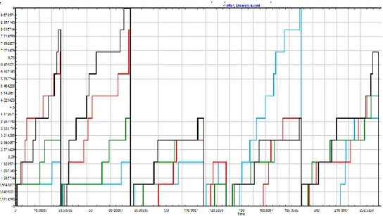
One requirement for obtaining a performance measure is that the system reaches a steady state. A system in steady state is when the system performance is independent of the starting conditions (Howard, 2007). This can be described as the system is performing as usual. Because we have stochastic input data the output data is also stochastic. The mean is then also a stochastic variable and if the simulation was run for an infinite time then that stochastic variable would converge to its true value by the law of larger numbers.

However, this is not possible so the mean is taken when a steady state has been reached. An example of steady state can be seen if figure 1, where the blue line is the mean inventory level and the red line is the inventory level. A steady state is reached when the blue line has levelled out. The decentralized model was run for 100,000 days and the centralized model was run for 10,000 days. The reason the centralized model was run a shorter time is that it is a more advanced model which takes a longer time to simulate. The optimization would take too long to finish.

Figure 1. Steady-state for a product.

0 214,2857 428,5714 642,8571 857,1429 1071,429 1285,714 1500 1714,286 1928,571 2142,857 2357,143 2571,429 2785,714 3000 0 2,083333 4,166667 6,25 8,333333 10,41667 12,5 14,58333 16,66667 18,75 20,83333 22,91667 25 27,08333 29,16667 31,25 33,33333 35,41667 37,5 39,58333 41,66667 43,75 45,83333 47,91667 50 Time Value

Plotter, Discrete Event

(19)

11

A major downside with optimization is that the model has to run many times which can take a long time and that the algorithm has an inability to tell when the best solution has been found. It is therefore important to run the optimization several times to make sure that the answers are the same so that one answer is not false or suboptimal.

2.2.5 Test and Refine the Model

Verification of the model should be done continuously and not after the entire model is finished according to Banks (1998). During the building of the models discussions with the stakeholders have continuously taken place when each step of the models has been verified. All requirements have also been discussed thoroughly.

To verify the simulation model Extendsim’s plotter was used to give a graphical representation on how the inventory levels changed over time. The plotter was also used to see if the joint replenishment was correctly modelled. This can be seen in figure 2. The graph displays the order queue for five products. When an order is made, all products queue should be emptied, which is also does. With this tool it was very easy to spot any errors and irregularities in the models.

Figure 2. Order queue.

Input Parameters

For the simulation model to run correctly several input parameters are necessary. The simulation model is linked to an Excel sheet where all parameters are entered, and then imported to the model at the start of the

(20)

12

simulation. See Appendix A and B to see how the Excel sheet is constructed.

The parameters are described below.

 A product’s demand over a year.

 Transportation time between the depots and the central warehouse as well as the lead time between the suppliers and the central warehouse.

 Wage cost of driver per hour as well as fuel cost per km for the transport between depots and central warehouse.

 Holding cost for all installations.

 Order cost when a depot orders units as well as when the central warehouse orders units from a supplier.

 Start position for the inventory level, here set to S, and the reorder point s.

During optimization, the starting position S and the reorder point s are changed for each simulation. All other parameters are held constant during optimization.

Output Parameters

In order to compare the models with each other, the following results are needed.

 The mean total cost per day for the system: The sum of holding, transportation and order costs.

 The number of orders per day:

o The number of times a depot has placed an order to the central warehouse or to the supplier for the decentralized model.

o The number of times the central warehouse places an order to the supplier.

 The number of transports per day: The number of transports between a depot and the central warehouse.

 Service levels: Service levels for all products in a depot.

After a simulation all results are exported to an Excel sheet which can be seen in Appendix C and D.

(21)

13

2.3 Credibility of This Master Thesis

When simulation models are used to evaluate a system it is important that the results and conclusions are correct. A high level of credibility is obtained when the following aspects are met: validity, reliability and objectivity (Björklund & Paulsson, 2003).

2.3.1 Validity

Validation is done to determine if the model is an accurate description of the real system (Banks, et al., 1998). Björklund and Paulsson (2003) define validity as “to what extent something really measures what it intends to measure”. It has to be done once the model has been created and before any tests can be completed. There are four general angles when validating a simulation model. Those are: performing self-validation, a third party performing the validation, validation is performed by the model user and validation is performed using a scoring model (Sargent, 2004).

Most validations are done by the developers themselves. However, the credibility will suffer because the developer’s objectivity is uncertain. To increase the objectivity it is important to let the users perform the validation (Sargent, 2004).

Another way to validate a model is to do a retrospective test. This is done by using historical data as input data and then to compare the results from the simulation model with the results from reality. This reveals if the model give better results than reality. The draw back with retrospective testing is that a correct result does not mean that the model provides good results in the future.

Validity of the Simulation Model

The validations of the models were done by its developers and its users. For this thesis a face validation test was done which involved showing the models to the users to make sure the behaviour of the models reflects the reality. All assumptions made in the models were also discussed in detail with them. Since there is not sufficient historical data a retrospective test could not be done.

We could compare the decentralized model with a similar model made by Arriva DK’s Operations Research Manager. The scenario simulated was with four products with different demand from the same supplier. The inventory system was controlled by a periodic review system policy with

(22)

14

joint replenishment. On Monday, Wednesday and Friday the inventory position are checked and an order is placed when a products inventory position declines to or falls below the reorder point. The lead time was set to one day and if an order was made on a Friday the units would arrive on the next Monday. The parameters that were checked were the average inventory levels, number of orders per day and all products’ service levels. The simulation time was set to 100000 days in order for the model to reach a steady state. The results of the simulations were almost identical and difference was less than a per cent.

For the centralized model, we could also use Arriva DK’s model to validate it. The centralized model is an extension of the decentralized model and it was possible to create a scenario where the two models behave in the same way. To make it work we had to adjust the central warehouse so that it works as a supplier. The central warehouse’s stock levels were changed to very high levels so that no stock outs could occur. This is because we have assumed that the supplier can always deliver. The transportation time between a depot and the central warehouse was set to 1 day. Besides these changes, all settings and parameters were the same. The results of the simulations were again almost identical and the difference was less than a per cent.

2.3.2 Reliability

Reliability describes how consistent a measure is (Björklund & Paulsson, 2003). A study has a high reliability if it can be performed multiple times with the same results. To obtain a high reliability, one has to ensure that the measurements do not contain any random errors and are as accurate as possible when gathering information.

Reliability in this Master’s Thesis

To achieve a high reliability in this master’s thesis all measurements during the simulations were taken in a steady state. As the input parameters used in the simulations are based on historical data, it is likely that the input data will change if a similar study is carried out in the future. Since the results are based on a variety of lead times, suppliers and demand patterns it is not likely that a change in them will affect the results significantly. Therefore the reliability in this study is regarded as high.

2.3.3 Objectivity

A study’s objectivity is defined as the extent to which the authors’ values influence the results. To increase a study’s objectivity it is important to clearly explain and motive choices made by the authors so that the reader

(23)

15

can form his own opinions. Objectivity is also further increased if sources are properly reproduced and avoiding distorting facts (Björklund & Paulsson, 2003).

Objectivity in this Master’s Thesis

We have kept our values and opinions aside throughout the project. All choices that we made have been explained thoroughly and based on facts to increase the objectivity. Furthermore, sources and references have been specified to support the objectivity. All assumptions made in the simulation models have been discussed with our supervisors to ensure a high objectivity. Since the data used in the simulations come from Arriva DK’s ERP-system the objectivity will not be an issue.

(24)

(25)

17

3. Theoretical Framework

The theoretical framework is presented in this chapter. Initially, a brief introduction to inventory control is presented. Then the ordering policy and the costs connected to the models are discussed. Finally, the theory behind a central warehouse and joint replenishment are discussed.

3.1 A Brief Introduction to Inventory Control

The flow of material and the costs it generate within an organization often holds great potential for improvement. Regularly, the objective of inventory control is to balance conflicting goals. To keep stock levels down but at the same time meet service level requirements.

This chapter aims to give background to existing inventory control theories and - concepts.

3.1.1 Basic Concepts

 Lead-time

o The time from the ordering decision until the ordered amount is available on shelf.

 Stock on hand

o The number of physical items available in the inventory facility.

 Backorder

o A record of a customer order that could not be immediately fulfilled and is waiting to be delivered.

 Inventory position/- level

o Inventory position = stock on hand + outstanding orders – backorders

o Inventory level = stock on hand - backorders

 Continuous - and Periodic review

o At continuous review the inventory position is monitored continuously. An order is triggered at the same time the inventory position reaches its reorder point.

o With periodic review the inventory position is only considered at certain given points in time. For example, once a day.

(26)

18

3.2 Ordering Policy

3.2.1 (s,S policy)

The ordering policy used by Arriva DK is the policy denoted (s,S). Where s

is the reorder point and S is the maximum inventory level. When the inventory position reaches s or below, an order is triggered up to position S. In case of continuous review and continuous demand, the inventory position can never decline under s. Because the reorder point, s, will always be hit exactly and at the same time the order will trigger. Also the order quantity will always be S-s units.

If the demand is not continuous and/or the review is periodic, the order quantity will vary. Under these conditions the inventory level and – position can, in theory, be anything between negative infinity and s when an order triggers.

A negative inventory level implies backorders. There are always costs connected to backorders, but they can be hard to quantify. Therefore, it is common to implement service constraints instead when determining the s and S parameters. This is an optimization problem where one wants to minimize the costs, and at the same time uphold a certain pre-determined service level.

(27)

19

3.3 Costs Connected to the Optimization Problem

3.3.1 Holding Costs

The dominating part of the holding cost is the cost for keeping capital tied up in inventory. The opportunity cost for this capital is usually a percentage of the total value of the inventory. The percentage is often derived from what return an alternative investment yields. Although there are other parameters such as financial risk to take into consideration. This makes the opportunity cost more complex to determine than setting it equal to the expected return of the alternative investment.

Other parts of the holding cost are for example: material handling, storage rent, insurance, damage and obsolescence. These costs should be allocated to different product types depending on their characteristics. Some product types take up more volume than others and should therefore carry a bigger part of the rent. Unless the rent is fixed which implies it is independent of the total volume.

3.3.2 Ordering Costs

When ordering from an outside supplier there are several costs connected with replenishment. The costs can either be fixed or variable. Fixed costs are independent of the number of units and – product types in an order. This can for example be costs for order forms and handling of invoices from the supplier.

The variable cost varies with the characteristics of an order. Often are these costs connected to the number of man-hours required for handling - and register the ordered material.

3.3.3 Backorder Costs

A backorder costs occurs when a demand cannot be met due to a shortage. There are two scenarios regarding a backorder.

1. The customer chooses another supplier and the sale is lost. In this case, the cost is the loss of the contribution the sale would have raised.

2. The order is backlogged and delivered at a later point in time. This usually means extra costs for administration, price discounts and transportation.

Both scenarios result in a loss of good will and reputation that may affect future sales.

(28)

20

Backorder costs are difficult to estimate and vary from situation to situation. Therefore, it is common to replace these costs with service constraints. This method is regarded to be simpler in many practical situations even though an adequate service level can be hard to determine. There are different definitions of service level and they may yield different results.

3.3.4 Service Constraints and - Levels

There are three main definitions of obtained service level. 1. Probability of no stock out per order cycle.

This definition can be interpreted as the probability that an order arrives before the stock on hand is finished. It is a very simple method to use, but has its disadvantages. The drawback is that the definition doesn’t consider the length of the order cycle. If the order quantity is large, it can cover the demand for a long period of time. Even if the definition yields a low service level, there is plenty of stock on hand most of the time due to the large order quantity. Similarly, with a short order cycle and small order quantities, the actual service level can be very low.

In case the customer only can order one unit at a time, the two other definitions are equivalent:

2. Fill rate – fraction of demand that can be satisfied immediately from stock on hand.

3. Ready rate – fraction of time with positive stock on hand.

Fill rate and ready rate gives a good picture of the actual service. They differ if the customer can order units in batches. Even if the stock on hand is positive, it might not be enough to cover large orders. This can result in a high ready rate but a low fill rate.

Service measures can be defined in many other ways than the three discussed above. How a company chooses to define its service is individual and could have a wide range of underlying factors. Although, when setting the service level it should be based on the expectation of the customers and weighted against the cost of maintaining the level of service.

3.4 Central Warehouse – Bundling and Distribution

(29)

21

in literature, it means replacing many smaller depots with one or a few larger central warehouses. According to Oskarsson et al (2013) the advantages of this strategy can be divided into two parts.

1. Cost reductions

- Lower fixed costs for personnel, inventories and administration due to the reduced number of warehouses.

- Reduced opportunity costs for capital tied up in safety stocks. - Easier to control and manage the flow of material from a

centralized position. 2. Increase in service

- Better precision in lead times due to the ability of keeping stock of a wider range of products than would be viable at a smaller warehouse.

- Faster and more precise delivery information to customers. A central warehouse can also act more as a wholesaler. The main task is bundling and distribution of products to the existing depots. This strategy aims to decrease the number of communication paths and relations needed within the supply chain, see figure 4 (Oskarsson, et al., 2013). Another important factor is the discounts outside suppliers’ offers when ordering large quantities (Arjan & Van Weele, 2010). By coordinating the demand of several depots, the same increase in service can be obtained as listed above.

(30)

22

However, Jonsson & Mattson (2011) argues that the need for bundling and aggregation may decrease. The increase in customer specific products and wide range of product variations makes the possibilities for aggregation scarcer. Also, the development within information technology makes it easier for suppliers to coordinate transports of different products to different recipients. This enables smaller order quantities to be carried out at reasonable transportation costs.

3.5 Coordinated Ordering

As discussed before, large costs are connected to procured material. Therefore it is worthwhile finding strategies to reduce the total cost of the procurement process. It is not uncommon that the indirect costs (e.g. order -, billing -, material handling - and holding costs) exceed the direct costs (e.g. cost price and transportation) (Jonsson & Mattson, 2011).

One strategy, to reduce these costs, is by coordinating the replenishments for different products. It can be advantageous to trigger orders for a group of items at the same time and thereby replenish them jointly. This strategy may enable discounts if the total order value from a certain supplier is higher than it otherwise would have been. It can also reduce the transportation costs because of fewer transports or by filling a truckload (Axsäter, 2006). The possible gains of applying coordinated ordering depend on the company’s specific situation and conditions. However, implementing a joint replenishment policy also raises difficulties, which will be discussed in “The joint replenishment problem”.

3.6 The Joint Replenishment Problem (JRP)

The joint replenishment problem (JRP) is well known and there are several different proposed approaches to it in the literature. The problem differs depending on the incentives, of the specific company, for practicing joint replenishment. The components of the problem vary whether the goal is to reduce order costs, - setup costs, - transportation costs or to achieve quantity discounts.

The main problem, however, is that the products that are jointly replenished get intertwined and affect one another’s reorder point. The system gets much more dynamic and there are an increase in parameters and restrictions to consider when determining the optimal batch quantities and reorder points.

(31)

23

This means that individually determined reorder points is not optimal to apply with a joint replenishment policy. Normally, individual reorder points are set so that a certain service level is upheld. If all products are ordered when one of the products reaches its reorder point, all other products are ordered too early. This results in a higher than intended service level, and thereby, higher inventory levels and - holding costs. (Axsäter, 2006)

Due to the increase in complexity a joint replenishment policy causes, the optimal solution is often very hard and time consuming to obtain from a deterministic model. Therefore, it is common to use heuristic methods or simulation when finding solutions to the JRP.

3.7 Mathematical Model

To gain a better understanding of the system dynamics it is advisable to describe it mathematically. Stefan Vidgren and Lars Bonke (2013) describe the current supply system at Arriva DK in the working paper An Exact Model to Evaluate Joint Replenishment at Arrivas Workshops.

With this mathematical model it is possible to calculate the total cost of a joint replenishment system. With a central warehouse, however, the model would have to expand significantly and consider even more parameters than it already does. It is a very demanding and advanced task to get such a model accurate.

This is the main reason to why simulation is the most suitable tool to evaluate a joint replenishment system of this dignity.

(32)

(33)

25

4. The Supply Chain Set-Up

This chapter aims to give a background to the real world set-up for the flow of spare parts at Arriva DK and describe the two set-ups used in the simulation study.

4.1 General Background

4.1.1 The Depots

Arriva DK has a total of 29 depots. The four depots, considered in the project, are all located in the same major city with the longest distance of 41, 2 kilometres between two of them as can be seen in table 1. Each of the depots has a fleet of busses allocated to them that they serve and repair on a daily basis, also on weekends.

Table 1 The distance and time between the depots (Google, 2013)

Depot 1 2 3 4 1 0 9,5 30 7 2 16 0 41,2 19,8 3 23 31 0 23,2 Kilometres 4 10 18 19 0 Minutes 4.1.2 The Suppliers

Most of the suppliers are local and can usually deliver an order the following weekday.

Table 2. Number of suppliers and products for each depot

Depot # Active Suppliers # Products

Depot 1 59 1907

Depot 2 54 1252

Depot 3 55 971

Depot 4 43 836

Total 90 3091

As can be seen in the table 2 above, there are a total of 90 unique suppliers that deliver to at least one of the four depots. A bus fleet consists of busses of different makes and models. The configuration of the bus fleet varies

(34)

26

from depot to depot and, with that, the demand for specific spare parts. That is the reason why not all suppliers deliver to all depots.

4.1.3 Demand

Demand is generated individually for every product at every depot and follows a Poisson process which is described in more detail in section 2.2.2.

4.2 Decentralized Set-Up (DC)

The DC set-up is constructed to reflect the flow of materials as of today.

Figure 5. The decentralized system.

4.2.1 DC - The Depots

A total of four depots are considered. The depots operate all days of the week. They all carry stock of spare parts and the replenishment of the inventory is managed separately at each location. Each depot can carry up to 10 different products.

(35)

27 4.2.2 DC - The Suppliers

All suppliers operate during the weekdays (Monday to Friday) and are closed on weekends. A maximum of eight different suppliers can be considered at the same time and each of them can carry up to five different products. They are assumed to have infinite stock of these products.

4.2.3 DC - Ordering Process

The depots’ order processes are independent of each other.

The (s,S) ordering policy is utilized for every product at all depots. Every product has its individual reorder point (s) and maximum inventory level (S).

All inventory positions are reviewed once every weekday, and not on weekends since the suppliers are closed.

An order is triggered when a product’s inventory position is at – or below its reorder point (s). This means that orders can be placed with suppliers once every weekday, when the review is done. Products with the same supplier are replenished jointly. This means that all products with the same supplier will be ordered when one of them reaches its reorder point.

The order quantities are matched so that each ordered product is at inventory position (S) when the order has been placed.

4.2.4 DC - Lead-Times and Transportation

The suppliers deliver the goods directly to the depots. The transportation cost is embedded in the cost price and are in a way independent of the volume or number of different products in an order.

The suppliers can always deliver a complete order on set lead-time but never on weekends. If an inbound delivery should coincide with a weekend, the goods will not be delivered until the Monday after.

4.2.5 DC - Costs and Constraints 4.2.5.1 Holding Cost

The holding cost is calculated for every product at every depot. The annual holding cost ( ) for product at depot is calculated through:

(36)

28 where * ̅ and

*The cost of capital ( ) used by Arriva DK is 7 %.

4.2.5.2 Order cost

The order cost depends on the number of different products in an order and is calculated through: where * ** *** and

*The constant cost for an order ( ) is derived from the average pay of personnel at the depots and man-hours spent on an order. This includes administration, receiving, controlling and putting the goods on shelves. The derived constant cost for an order is 110 DKK.

**The billing cost ( ) is set to 10 DKK per order, as estimated by Arriva DK.

***The variable cost ( ) is the extra cost that occurs for every different product in an order. This cost is estimated by Arriva DK to be 15 DKK.

(37)

29

With the above-mentioned costs, the order cost function can be written:

4.2.5.3 Backorders

If a demand cannot be met immediately due to stock-out at the depot, the customer will wait and be served when the stock is replenished. A backlogged customer is never lost and there are no extra costs connected to them. Instead, service constraints are used to ensure an adequate level of service.

4.2.5.4 Service Constraints

The ready rate is measured individually for all products at all depots and the service level is set to 99 %.

This means that all products should have positive stock on hand at least 99 % of the time.

(38)

30

4.3 Centralized Set-Up (CW)

The CW set-up introduces a central warehouse to the supply chain. 4.3.1 CW - The Depots

The set-up for depots 2, 3 and 4 are the same as in the DC set-up, see section 4.2.1.

Depot 1 now also functions as a central warehouse, see section 4.3.3.

4.3.2 CW - The Suppliers

The set-up for the suppliers is the same as in the DC set-up, see section 4.2.2.

(39)

31 4.3.3 CW – Depot 1/The Central Warehouse

Depot 1 functions as a central warehouse while still continuing to serve its own bus fleet. It can generate demand for up to 10 different products but does not carry stock for any of the products. Instead, the demand is satisfied directly and immediately by the central warehouse stock.

The central warehouse operates all days of the week and can keep a maximum of 40 different products in stock.

4.3.4 CW - Ordering Process

Depots 2, 3 and 4 replenish their inventories from the central warehouse while the central warehouse replenishes its inventory from the outside suppliers.

The Central Warehouse

The order process for the central warehouse is exactly the same as for a single depot in the DC set-up.

 (s, S) policy

 Joint (supplier-dependent) replenishment

 No reviews or orders on weekends

See section 4.2.3 for details.

The Depots

Depot 1 does not carry any stock and places therefore never any orders. Depots 2, 3 and 4 utilizes the (s,S) policy and only order from the central warehouse.

Because the central warehouse operates all days of the week, orders can be placed on all days. This means that reviews of a products inventory position in a depot is made twice every day as well.

The replenishment is not supplier-dependent. When a depot places an order with the central warehouse, all products at that depot will be replenished jointly.

Contrary to the suppliers, the central warehouse does not have infinite stock. This means that a depots’ ordered quantity could exceed the available stock. If so, the depots’ ordered quantity is changed to match whatever quantity is

(40)

32

available at the central warehouse. This policy makes it impossible for orders to be backlogged at the central warehouse.

4.3.5 CW – Lead-Times and Transportation From Suppliers to Central Warehouse

The suppliers always deliver a complete order on a set lead-time but never on weekends. If an inbound delivery date should coincide with a Saturday or a Sunday the goods will be delivered on the following Monday.

From Central Warehouse to Depots

There is one van assigned to carry out the transports between the central warehouse and the depots. The van operates all days of the week.

The lead-time depends on the time it takes to drive between the central warehouse and the depot in question. Also, time for picking – and loading of the goods is added to the total lead-time. The time for picking and loading is set to two hours.

4.3.6 CW – Costs and Constraints 4.3.6.1 Holding Cost

The holding cost is calculated individually for every product at the depots and the central warehouse.

The annual holding cost ( ) is calculated in exactly the same way as for the DC set-up:

̅

See section 4.2.5.1 for details.

4.3.6.2 Order Cost

The cost for an order (C) to an outside supplier is calculated exactly as in the DC set-up:

See section 4.2.5.2 for details.

Arriva DK does not practice internal billing. Hence, the order cost between a depot and the central warehouse will be:

(41)

33

The actual values of , and is estimated to be the same for both set-ups:

and

4.3.6.3 Transportation Cost

The cost for a transport ( ), between the central warehouse and depot j, consists of two parts: hourly pay for the chauffeur (p) and fuel cost per kilometre (g). Every transport is considered to be a round trip.

( ) where,

( ) and,

( )

The actual values of the hourly pay (p) and fuel cost (g) are based on costs

for a similar, existing, transport operation within Arriva DK:

The distance and driving time between the central warehouse and the depots were obtained from Google MapsTM (Google, 2013).

Table 3. Transportation distance and time.

Depot 2 3 4

(hours) 0,27 0,38 0,17

(42)

34

With these parameter values, the cost per transport for each depot is: *

( ) ( ) ( )

*There is no transportation costs associated with satisfying the demand Depot 1 generates. The central warehouse stock is assumed to be directly available to Depot 1.

4.3.6.4 Backorders

As discussed in section 4.3.4, backorders are not allowed at the central

warehouse.

If a demand cannot be met immediately due to stock-out at the depot, the customer will wait and be served when the stock is replenished. A backlogged customer is never lost and there are no extra costs connected to them. Instead, service constraints are used to ensure an adequate level of service.

4.3.6.5 Service Constraints

The ready rate is measured individually for every product at every depot and the service level is set to 99 %.

There are no individual service constraints for the central warehouse since it is only the level of service to external costumers that is of interest in this project.

(43)

35

5. Simulation Scenarios

In this chapter the results from the different simulation scenarios are presented. In order to see if a central warehouse is better than a decentralized model; different scenarios have been created to get different views and outputs.

5.1 Scenario 1

5.1.1 Description

This scenario was constructed to get an overall performance indicator of the two models when optimized.

Eight products from eight different suppliers were selected (one product per supplier). The parameters, such as demand, cost price and lead time, are all based on real historical data extracted from Arriva DK’s ERP-system. The lead time from the suppliers is set to one day.

The purpose of this scenario is to gain knowledge of the total costs for the two systems and how the costs are allocated.

5.1.1 Result and Discussion

Table 4 below presents the results from the simulations of the models.

Table 4. Results from the simulations.

Costs/Model DC CW

Costs/year

Mean holding cost 24,96 33,19

Order cost 20,82 21,54

Transportation cost 0 4,62

Total Cost 45,78 59,35

Orders/year

Number of orders to suppliers 56,28 32,45

Number of orders to the central warehouse 0 18,03

Total 56,28 50,48

The most distinct difference is the holding cost. With joint replenishment and shorter lead times between the CW and the depots, the depot can have

(44)

36

less inventory and keep the same service levels as before. This reduction is, however not enough to compensate for the increased inventory levels at the CW for this scenario. This could have its explanation in that the order cost, together with the transportation cost, between CW and depots is too high to fully exploit the shorter lead times. The central warehouse has to hold large quantities in stock to be able to supply the depots. Stock that otherwise would be at the suppliers.

The total number of orders is lower for the CW but at the same time the order cost is higher compared to DC. That is because more products are ordered at the same time with a CW than without. The cost for ordering eight products is more than twice as high as for ordering one product.

The transportation stands for about 10% of the total cost in the CW model. This is a service otherwise provided by the suppliers. The transportation cost is not entirely fair because in the real world the cost would be distributed on several products. It depends on the number of orders not the number of products.

Table 5 below presents the key figures and key differences.

Table 5. Key figures from the simulations.

Key figures /year

TCDC 16707,9

TCCW 21660,9

Difference in TC 4952,9

TCCW/TCDC 1,296

Total purchase price of demanded units 638262,6

TCCW/TCDC with total purchase price 1,0076

Discount needed on cost price for the same total cost 0,78%

Difference of orders to suppliers 57,66%

The model with a central warehouse has a total cost of almost 30% more than the decentralized model. In a year, this corresponds to almost 5000 DKK. However, if you factor in the total purchase price of demanded units, the difference is very small. The model with the central warehouse is only 0, 76% more expensive.

The number of orders to suppliers with a central warehouse is almost half that without a central warehouse. With a central warehouse, the suppliers

(45)

37

only have to deliver to one place instead of four. The central warehouse will therefore order larger batches but not as often. This is a significant reduction and should motivate a discount on the cost price which has been discussed with the Purchasing Manager. Discounts on the cost price of 0, 8 % have to be achieved for the two models to have the same total cost.

From this scenario it is hard to get a definitive answer whether a central warehouse is a better solution than a decentralized model so more scenarios have to be considered.

5.2 Scenario 2

5.2.1 Description

In this scenario we examined how the number of different suppliers as well as the demand affected the results. In order to see how the number of suppliers affects the result we ran four different scenarios, which can be seen in table 6.

Table 6. The scenarios that will be simulated.

Scenario 1: 1 Supplier - 8 Products

Scenario 2: 2 Suppliers - 4+4 Products

Scenario 3: 4 Suppliers - 2+2+2+2 Products

Scenario 4: 8 Suppliers - 1+1+1+1+1+1+1+1 Products

All products have the same demand and cost price in each scenario. However in order to see how demand affected the results, each scenario were run two times with different demand. The first time the demand was set to 50 products per year and the second time the demand was set to 100 products per year. The reason we chose these demands was that they reflected the demand for an average product and spare parts have generally low demand. The cost price was set to 1000 DKK. The lead time for units shipped from a supplier was set to one day.

5.2.2 Result for the scenario with 50 in demand

(46)

38

Table 7. 50 in demand and 1000 DKK in cost price

Scenarios Model Holding cost/day

Order cost/day

Transportation

cost/day _cost/dayTotal 1 Supplier DC 32,41 28,29 0 60,7 CW 43,34 34,30 11,67 89,32 2 Suppliers DC 35,15 31,50 0 66,64 CW 50,22 32,59 9,71 92,52 4 Suppliers DC 40,67 33,53 0 74,20 CW 48,46 40,39 10,49 99,34 8 Suppliers DC 44,67 41,99 0 86,66 CW 49,15 48,30 10,66 108,07

The total cost is higher for the centralized model for all scenarios. One can also see that when the number of suppliers increases the difference becomes smaller. The differences in holding cost between the models are much less with 8 suppliers than with 1 supplier. For the centralized model, the stock levels at the depots are the same no matter how many suppliers are used thanks to the use of a central warehouse. Due to the benefits of using joint replenishment the maximum stock levels can be lowered resulting in lower holding costs.

The difference in order cost decreases as well when more suppliers are used. This is also a result of using a central warehouse. The number of suppliers has no effect when a depot places an order. On the other hand the transportation cost, which is added with a central warehouse accounts for a large part of the total cost. In table 8 below the number of orders are presented. In table 8 below the number of orders are presented.