VTI rapport 1078A Utgivningsår 2021 vti.se/publikationer
Effects of incidents on
motorways
A proposed methodology for estimating and
predicting demand, duration and capacity for
incident management
Ellen Grumert Viktor Bernhardsson Per Strömgren David Gundlegård Johan Olstam Joakim Ekström Rasmus RingdahlVTI rapport 1078A
Effects of incidents on motorways
A proposed methodology for estimating and
predicting demand, duration and capacity for
incident management
Ellen Grumert
Viktor Bernhardsson
Per Strömgren
David Gundlegård
Johan Olstam
Joakim Ekström
Rasmus Ringdahl
Author: Ellen Grumert, VTI, Viktor Bernhardsson, VTI, Per Strömgren, Movea, David Gundlegård, LiU, Johan Olstam, VTI, Joakim Ekström, LiU, Rasmus Ringdahl, LiU Reg. No., VTI: 2017/0669
Publication: VTI rapport 1078A Published by VTI, 2021
Publikationsuppgifter – Publication Information
Titel/TitleIncidenters påverkan på motorvägar – Ett förslag på metodik för att skatta och prediktera trafikefterfrågan, incidentens varaktighet och kapacitet för incidenthantering/
Effects of incidents on motorways - A proposed methodology for estimating and predicting demand, duration and capacity for incident management
Författare/Author
Ellen Grumert (VTI, http://orcid.org/0000-0001-5531-0274)
Viktor Bernhardsson (VTI, https://orcid.org/0000-0003-0767-5169) Per Strömgren (Movea)
David Gundlegård (Linköpings universitet, https://orcid.org/0000-0002-5961-5136) Johan Olstam (VTI, https://orcid.org/0000-0002-0336-6943)
Joakim Ekström (Linköpings universitet, https://orcid.org/0000-0002-1367-6793) Rasmus Ringdahl (Linköpings universitet)
Utgivare/Publisher
VTI, Statens väg- och transportforskningsinstitut
Swedish National Road and Transport Research Institute (VTI)
www.vti.se/
Serie och nr/Publication No.
VTI rapport 1078A
Utgivningsår/Published
2021
VTI:s diarienr/Reg. No., VTI
2017/0669
ISSN
0347–6030
Projektnamn/Project
Incidenters inverkan på kapacitet och trafikföring / Capacity at incidents
Uppdragsgivare/Commissioned by
Trafikverket / Swedish Transport Administration
Språk/Language
Engelska / English
Antal sidor/No. of pages
Sammanfattning
Incidenters påverkan på motorvägar – Ett förslag på metodik för att skatta och prediktera trafikefterfrågan, incidentens varaktighet och kapacitet för incidenthantering
Ellen Grumert (VTI), Viktor Bernhardsson (VTI), Per Strömgren (Movea), David Gundlegård (LiU), Johan Olstam (VTI), Joakim Ekström (LiU), Rasmus Ringdahl (LiU)
Effektiv incidenthantering är viktigt då man vill minimera trängsel till följd av incidenter. Prediktering av framtida trafikförhållanden vid incidentplatsen och dess omgivande vägnät, tillsammans med en uppskattning av incidentens varaktighet, kan användas för att få ökad kunskap om nuvarande och framtida utveckling till följd av incidenter med specifika egenskaper.
Syftet med denna studie är att föreslå metoder för att skatta kapacitet, varaktighet och efterfrågan för incidenter med olika egenskaper, samt att undersöka hur detaljnivån och möjligheten att identifiera förklaringsvariabler för incidenter med liknande egenskaper givet tillgängliga datakällor påverkar de föreslagna metoderna. Kunskapen som erhållits i projektet avsedd att användas för incidenthantering. Rapporten presenterar en metodik för att prediktera kapacitet, trafikefterfrågan och varaktigheten av incidenter när ingen av parametrarna är kända. Den föreslagna metodiken kan användas för att förse trafikmodeller med input då syftet är att utföra scenariobaserad analys och realtidspredikteringar som ska användas i beslutsprocessen för trafikledning/styrning vid incidenter, men också för att förutsäga förändrade restider till följd av incidenten som skulle kunna kommuniceras till trafikanter.
En motorvägssträcka söder om Stockholm används som fallstudieområde för att föreslå metoder för att prediktera varaktighet, kapacitet och efterfrågan vid incidenter baserat på tillgängligheten av data. Den föreslagna metodiken utvärderas genom att använda de predikterade variablerna som input i en
scenariobaserad analys med två kömodeller.
Resultaten visar att tillförlitligheten av predikteringarna av de tre variablerna har stor inverkan på den predikterade köutbredningen. Fel i predikteringen av kapacitet och efterfrågan verkar ha större effekt på skillnaden mellan predikterad och observerad köutbredning än fel i predikteringen av tidsåtgång för incidenthanteringen. Trafikmodellsresultaten visar att det är svårt att skatta generella samband mellan förklaringsvariabler också även för likvärdiga incidenter.
Nyckelord
Kapacitet, olycka, incident, motorväg, efterfrågemodellering, tidsåtgång för incidenthantering, kömodellering, trafikföring
Abstract
Effects of incidents on motorways – A proposed methodology for estimating and predicting demand, duration and capacity for incident management
Ellen Grumert (VTI), Viktor Bernhardsson (VTI), Per Strömgren (Movea), David Gundlegård (LiU), Johan Olstam (VTI), Joakim Ekström (LiU), Rasmus Ringdahl (LiU)
Effective traffic incident management is important to minimize negative impacts of congestion caused by incidents. Predictions of the traffic state at the incident site and its surrounding road network, together with an estimate of incident duration, can be used to get increased knowledge about current and future incident characteristics.
The aim is to propose methods for estimating capacity, duration and demand profiles in case of an incident, and to explore how the level of detail and the possibility to identify explanatory variables for incidents with similar characteristics given currently available data sources affects the proposed methods. The knowledge obtained within the project is intended to be used for incident management. The report presents a methodology for predicting capacity, traffic demand, and incident duration, when none of the parameters are known. The proposed methods can be used as input to traffic models, when the purpose is to perform scenario-based analysis and real-time predictions to be used in the decision-making processes for traffic management/control, but also for predicting travel times which can be communicated to road users.
A motorway use-case study area south of Stockholm is used to propose methods for predicting incident duration, capacity and demand profiles based on the availability of data. The methodology is evaluated by using the predicted variables as input in a scenario-based analysis with two queue models.
The results show that the accuracy of the predicted variables have a large impact on the predicted queue propagation. Inaccurate predictions of capacity and demand seems to have a larger impact on the error between the observed and the predicted queue propagation compared to the incident duration. Results from the traffic modelling show that it is challenging to estimate generic relationships between available explanatory variables and the traffic conditions at the incident site, even for incident with similar characteristics.
Keywords
Capacity, accident incident, motorway demand prediction, incident duration, queue modelling, traffic management
Preface
This report present results from the project Capacity at incidents funded by the Swedish Transport Administration via Centre for Traffic Research (CTR). The project has been carried out by Ellen Grumert, Viktor Bernhardsson and Johan Olstam at the Swedish National Road and Transport Research Institute (VTI), Joakim Ekström, David Gundlegård and Rasmus Ringdahl at Linköping university (LiU) and Per Strömgren and Axel Ericsson at Movea. The reference group have consisted of persons from the Swedish Transport Administration (Per-Olof Svensk), the Stockholm traffic control centre TrafikStockholm (Alexander Nilsson, Kristofer Svensson and Otto Åstrand) and the Royal Institute of Technology (Athina Tympakianaki and Erik Jenelius). Per-Olof Svensk have been the contact person at the Swedish Transport Administration.
Linköping, November 2020 Ellen Grumert
Kvalitetsgranskning
Granskningsseminarium har genomförts 19 januari 2021 där Erik Jenelius var lektör. Ellen Grumert har genomfört justeringar av slutligt rapportmanus. Forskningschef Magnus Berglund har därefter granskat och godkänt publikationen för publicering 15 februari 2021. De slutsatser och
rekommendationer som uttrycks är författarnas egna och speglar inte nödvändigtvis myndigheten VTI:s uppfattning.
Quality review
A review seminar was held on 19 January 2021, with Erik Jenelius as the reviewer. Ellen Grumert has adjusted the final report. Research Director Magnus Berglund has thereafter reviewed and approved the report for publication on 15 February 2021. The conclusions and recommendations in the report are those of the authors and do not necessarily reflect the views of VTI as a government agency.
Table of Contents
Publikationsuppgifter – Publication Information ...3
Quality review ...7
Kvalitetsgranskning ...7
1. Introduction ...10
1.1. Purpose and aim ...11
1.2. Methodology framework ...11
1.3. Delimitations ...12
1.4. Structure of the report ...13
2. Description of the study case and available data sources ...14
3. Estimation of capacity and fundamental diagram ...18
3.1. Identification of breakdowns and periods with stationary traffic conditions (quantitative approach) ...19
3.1.1. Identification of changes in the traffic state through identification of periods with stationary traffic conditions ...20
3.1.2. Identification of traffic breakdowns ...21
3.2. Identification of capacity and throughput observations (qualitative approach) ...23
3.3. Estimation of the capacity distribution ...25
3.4. Estimation of the parameters of the fundamental diagram ...26
4. Estimation of duration of incidents ...29
4.1. Data collection ...29
4.2. Analysis ...29
4.3. Summary of findings ...32
5. Demand estimation and prediction ...34
5.1. Data processing and characteristics ...35
5.2. Prediction method ...38
5.3. Results ...38
5.4. Discussion ...41
6. Evaluation of methodology through traffic modelling of incidents ...42
6.1. Investigated incidents ...43
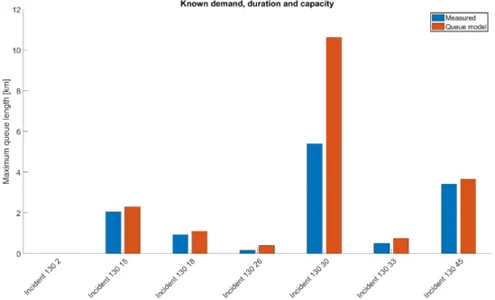
6.2. Traffic model verification – known demand, duration and capacity ...51
6.3. Predicted demand ...55
6.4. Predicted duration ...58
6.5. Predicted capacity ...61
6.6. Predicted demand, duration and capacity ...62
6.7. Application of methodology in real-time incident management ...65
Conclusions and future research needs ...68
References ...71
Appendix A – Incident duration for accidents and objects on the roadway ...73
Appendix B – Traffic modelleing results for all incidents ...76
Incident 130 2 ...76
Incident 130 15 ...78
Incident 130 26 ...84
Incident 130 30 ...87
Incident 130 33 ...90
1.
Introduction
Incident management aims to improve traffic conditions on the incident site, both with in terms of road safety and traffic efficiency. Ensuring the safety of road users and rescue personnel is, of course, the most important task. However, the road users can experience long travel times and fast backwards propagating queues, resulting in large negative impacts on traffic efficiency and costs for the society in terms of delays. Therefore, an efficient traffic management, not compromising road safety, is of great importance for larger cities with frequently observed breakdowns.
To achieve an efficient incident management, information both about the current and the future traffic state is needed. Predictions of the future traffic state at the incident site and its surrounding road network, together with an estimate of the incident duration, can then be used for travel time forecasts and prediction of queue length and queue-propagation speed at different time instants. The duration of an incident can be divided into the following phases: discovery, verification, initial response, scene management, and recovery (Ebner m.fl., 2011). After the recovery phase the incident scene is cleaned and the road can be fully opened again, but it will still take some time to restore the traffic conditions to normality, which is the last phase in the traffic incident management phases according to Ebner m.fl. (2011). As a conclusion, when an incident occurs it is essential to contribute with predictions and answers to the following issues, both for incident management and to provide as accurate information as possible to road users (see Figure 1 for an illustration in the space -time domain):
1. How much time is required for the incident management? 2. Will there be queue propagation?
3. How far in the network will the queue reach?
4. How much time is needed for restoration to normality?
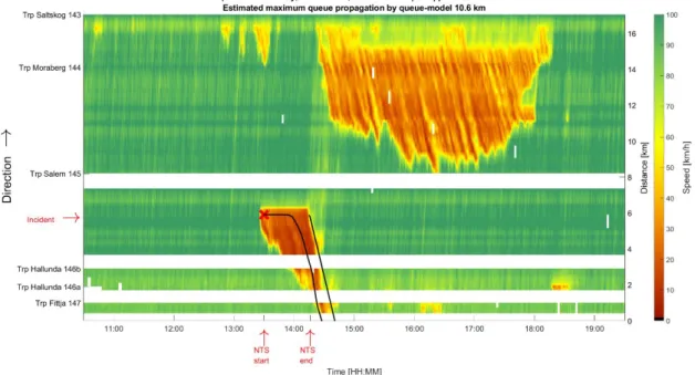
Figure 1. Illustration of an incident and what uncertain variables that need to be predicted in order to predict effects of incidents, either in real-time or in a scenario-based evaluation. The observed speeds ranges from 0 (red) to 100 (green) km/h. The time together with the start and the end of the incident is given on the y-axis and the location is given on the x-axis.
Question 1 highly depend on the severity and magnitude of the incident. This question requires detailed data on incident characteristics and durations of previous incidents to enable accurate predictions. Question 2 - 4 require estimates and predictions of the traffic states and how they
propagate in time and space. Traffic state predictions are commonly based on measurements of the current and past traffic situation, which together with a traffic model can be used to predict how the future, not yet known, traffic state change over time and/or space. Knowledge of incident
characteristics and the effect these will have on incident duration and the traffic characteristics, such as capacity, free flow speed, etc, is thus essential for a correct prediction. Further, an estimate of the demand at the time of the incident, and the near future, is required to predict how the traffic state will develop over time, given the predicted inflow profile.
One problem in analyzes of the traffic efficiency and capacity effects of incidents is that essential information about the incident characteristics and the incident management actions is not saved, alternatively not saved with a sufficient level of detail. Examples of information that is commonly not saved are how many lanes an incident blocks or which lanes that are closed by the traffic management center, over how large distances lanes are blocked or closed, as well as durations of the incident phases, e.g. time from knowledge of the incident to arrival of rescue leaders, rescue vehicles, time required for partial progress in incident management, such as medical interventions, salvage, etc. All this information is essential in the development of decision support for incident management to ensure that the best strategies are used together. Collection of this type of information needs to be done through automatic logging or with the help of outside observers as traffic managers, roadside assistance and rescue personnel need to have full focus on taking care of the incident.
1.1. Purpose and aim
The purpose of this work is to contribute with increased knowledge about different types of traffic incidents and how traffic performance is affected when an incident occurs by using available data sources with different levels of detail.
The aim is to propose methods for estimating capacity, duration and demand profiles in case of an incident, and to explore how the level of detail and the possibility to identify explanatory variables for incidents with similar characteristics given currently available data sources affects the proposed methods.
In a broader perspective, the knowledge obtained within the project is intended to be used for incident management, to be able to apply effective actions to prevent heavy congestion and improve traffic efficiency.
1.2. Methodology framework
The proposed methodology consists of several parts. Figure 2 gives an overview of the methodology framework, including possible application areas. In the figure, it is illustrated how the resulting output from the proposed methodology can be used as input to different application areas. However, to be utilized in each application area additional methods might be required. The development of such methods is outside of the scope of this study.
First, the available data sources have been identified through discussions with the Swedish Transport Administration, Trafik Stockholm and the included project partners (VTI, LiU, Movea, and KTH). Quantitative methods (1.1) are applied to estimate the traffic state, duration of incidents, demand profiles, etc. for different incident types and qualitative methods (1.2) are applied to investigate if more details can be included from individual incidents. The results from 1.1 and 1.2 is used in 2 to analyze if it is possible to identify different traffic characteristics, demand profiles and incident durations for a number of possible explanatory variables. To evaluate the performance of the applied methodology, the results from 1.1, 1.2 and 2 is used in a scenario-based analysis (3.2) by applying two different traffic models: a version of the queue model developed in PRIMA (Taylor m.fl., 2017, Olstam m.fl., 2015) and the Cell Transmission Model (CTM), which is a well-known first-order macroscopic traffic simulation model (Daganzo, 1994). The queue model is especially designed for
incidents and its modelling of different incident phases, why the focus is on the incident location and the queue propagation without modeling of the traffic state extent in the space domain, while the CTM model is a time and space discrete model, meaning that it does also have a spatial representation of the traffic states. A road stretch south of Stockholm with frequently observed incidents and accidents are used both to develop and evaluate the methodology. The performance of the proposed methods for estimating duration, demand and capacity effects are evaluated by predicting the queue length using the traffic models and compare it to observed queue lengths from measurements for seven incidents, corresponding to the most common incident type, i.e. scenario-based analysis. Sensitivity analysis is performed to investigate how sensitive the predictions of queue length are too uncertainties in the predictions of duration, demand and capacity. The main considered application area for the proposed methodology is in this study delimited to real-time incident management (3.4), but also scenario-based analysis (3.2) is highly relevant since it is used to evaluate the performance of the proposed
methodology for historical incidents.
Figure 2 Overview of the methodology framework
The estimations and predictions of capacity, demand profiles and incident duration is dependent on the availability of historical and real-time data. In real-time incident management the estimation of queue length, travel times, etc. must be performed online given a continuous flow of data, however, the predictions and estimation of specific variables, such as capacity, demand profiles and incident
durations, can be based only on historical data and offline predictions and estimations. In that case, the real-time data is used only to find the most suitable capacity estimate, demand profile and incident duration based on the available information at the incident site. It is possible to enhance the
predictions and estimations of the specific variables in real-time by performing online predictions of future traffic conditions if the availability of data is enough to perform such predictions and the data can be delivered without a considerable delay. Additionally, the online methods used for prediction has to be fast enough to deliver real-time predictions as input to the incident management.
1.3. Delimitations
The focus of the study is on the proposed methodology for predicting and estimating traffic characteristics, duration, and demand profiles at incidents. The study does not intend to develop methods for the suggested application areas in Figure 2. Instead, this study is delimited to an investigation of the performance of the proposed methodology for real-time incident management (application area 3.4: Real-time estimation) by performing a scenario-based analysis of past incidents (application area 3.2: Scenario-based analysis). The real-time incident management framework is investigated using already existing methods.
This work is limited to incidents on urban motorways and the empirical observations and investigations are based on data from a 15 km long urban motorway stretch south of Stockholm, Sweden. The focus has been on the incident category stopped vehicles, since the other types of incident are less frequent, resulting in too few observations to draw any conclusions on possible explanatory variables. Data is limited to observations from 2017. However, it is believed that the proposed methodology can be used for other road types with similar data set.
The project does not aim to develop a decision support system for incident management. The project results should instead be seen as a proposed methodology that can be used in a future implementation of such a decision support system.
The developed relationships between traffic characteristics, demand and duration, and the identified explanatory variables should not be seen as descriptive for all roads with similar road and traffic characteristics, since more research and a larger data set is needed to conclude on these relationships.
1.4. Structure of the report
First, a description of the case study road stretch and the available traffic and incident for this road stretch is presented in Chapter 2. Analysis and methods for estimating capacity during incidents, incident duration, and demand are then presented in chapter 3,4 and 5, respectively. The proposed methodology is evaluated in chapter 6, by using the predicted capacity, duration and demand for seven representative incidents as input in a traffic model for predicting queue propagation at incidents. An outline of how the proposed methodology can be used in incident management is also presented. Finally, in Chapter 7, conclusions and suggestions for further research are given.
2.
Description of the study case and available data sources
A case study-based approach has been used to investigate how currently available data sources can be used to estimate capacity, duration and demand in connection with incidents data. The case study area is chosen based on a set of criteria: (1) the road network should have a straightforward design with few on- and off-ramps and longer stretches with homogenous road conditions to be able to isolate effects of incidents from effects caused by regular congestion, (2) incidents should be a common phenomenon along the road stretch, (3) more than one data sources should be available, (4) the available data sources should include enough measurements to estimate one or more of the traffic state, duration of incidents, demand profiles, (5) if possible, detailed information about incidents should be included to increase the knowledge on specific traffic characteristics for the investigated incidents. The E4 South of Stockholm, between Södertälje and Fittja, just before the inner city of Stockholm, fulfill the
requirements and have been chosen as the case study area. The considered road stretch is a 15 km long motorway stretch with three on- and off-ramp locations, see Figure 3. The road stretch consists of large homogenous road segments with three lanes and a speed limit of 100 km/h. At the on- and off-ramps the number of lanes varies from two to four. At Hallunda and further towards Stockholm city the speed limit is reduced to 80 km/h. Congestion is frequently observed during high traffic flows both in the southbound and the northbound direction because of merging maneuvers and lane-drops at the on- and off-ramp locations. Additionally, incidents are common due to the high speed limit together with a high traffic flow and a narrow road with three lanes and limited road side, and sometimes much curvature and steep slopes.
Figure 3. Considered road stretch, E4 South of Stockholm, between Södertälje and Fittja, marked with blue, both the northbound and southbound direction were included in the analysis.
The available data sources are taken from
• detector data incorporated in the Motorway Control System (MCS) • incident data from Nationellt Trafikledningsstöd (NTS)
• accident data from the Swedish Traffic Accident Data Acquisition (STRADA), and • detailed incident and accident reports (Vägvakt).
The year 2017 is chosen for collection of MCS, NTS and STRADA data. Vägvakt reports are
unfortunately no longer collected and the data therefore consists of older data covering the years 2010 to 2013.
The MCS detector data consists of speed and flow measurements on individual lanes. 116 densely placed detectors are located on the considered road stretch, 60 in the northbound direction and 56 in the southbound direction. Figure 4 gives an overview of the detector locations. The measurements (counts of vehicles and mean speed) are collected over one-minute periods. Additionally, information about lane-closure is included since an incident is almost always followed by a closure of one or more lanes. The MCS data is used in the quantitative methods to estimate the traffic state and demand profiles and to detect days with incidents.
Figure 4. Overview of detector locations along the considered road stretch, E4 South of Stockholm, between Södertälje and Fittja (Löfgren, 2014).
Detailed incident data is available through the NTS and STRADA databases for the whole considered road stretch. In the NTS database information about individual incidents and accidents are available. The STRADA database includes descriptions of accidents that has resulted in personal injuries. The information is gathered from the police and the healthcare. The information in STRADA is available for everyone on an aggregated level, but more detailed information is available for those actively involved in traffic safety research. The incident data is used to identify individual incidents, to categorize the incidents into subgroups and to identify possible explanatory variables for how the capacity and other important traffic characteristics are affected by different types of incidents. The available information from the NTS and the STRADA database is summarized in Table 1.
Table 1. Description of available data from the NTS and the STRADA database.
Data Description
NT
S
ID The specific id of an incident
Date The date of the incident
Time The time of the incident
Event Defines the type of incident, accident/stopped vehicle/dropped load/burning vehicle/towing
Source The source from where the information about the incident have been collected. This might for example be the road assistance personnel.
Location Information about the location, such as the gps coordinates of the detector (portal) associated with the incident, road direction and the on- and off-ramp location if the
incident occur at such location. Notes
Can include information about included vehicle types, number of involved vehicles, road assistance, detailed location of the involved vehicles (lane location, number of blocked lanes, on-/off-ramp blocking, etc. The details in the available information varies from nothing to many details depending on the source of information.
Lane number The lane where the incident occurs, ranging from 1 to 3 on a three-lane motorway.
ST
RADA
ID The specific id of an accident resulting in personal injuries
Date The date of the accident
Time The time of the accident
Detector The gps coordinates of the detector (portal) associated with the accident
Event Information about the accident, a more or less detailed description of the course of the accident.
Injury severity The severity of an injury, including slight (swedish: lindrig) and severe (swedish: svår) injuries.
Vehicle type Type of vehicle included in the accident
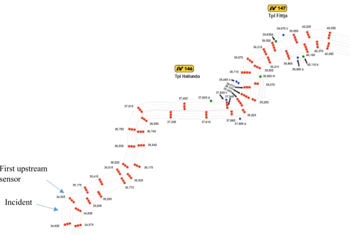
The incident documentation from Vägvakt consists of older incident data on a detailed level in the form of disturbance reports from individual incidents. The disturbance reports include incidents from the motorway situated between interchange Hallunda (Interchange 146 in Figure 4) and interchange Moraberg (Interchange 144 in Figure 4). The reports contain information about alarm type, times, location, event type, cause of incident, degree of blockage, interventions and other comments, see an example of a disturbance report (in Swedish) in Figure 5.
3.
Estimation of capacity and fundamental diagram
Some parameters describing the traffic characteristics are of great importance when evaluating the effects of an incident. These are capacity, free flow speed, critical density and the shockwave speed. The capacity indicates how many vehicles per hours that can be served at the incident site. The
capacity will obviously be affected by an incident as a result of partially or fully blocking of lanes. A first guess would be to only reduce the capacity with the number of lanes that are not available, however, this is usually not the case. The type of incident, as well as the severity, number of rescue units, etc. will all have an impact on the resulting capacity. The CEDR project Pro-Active Incident Management (PRIMA) (Nitsche m.fl., 2016) concluded that there is limited knowledge on how much the capacity is affected by different types of incidents.
The free flow speed is the average speed at free-flowing traffic conditions, corresponding to the
average speed at low traffic flows. At a homogenous motorway stretch this is usually close to the actual speed limit on the road. However, when an incident occur vehicles might have a different desired speed, even if there is no congestion on the incident site. Commonly, the drivers reduce the speed to adapt to the prevailing traffic conditions at the incident site, due to e.g. a sense of insecurity, limited lateral space, for safety-related reasons and concerns for people and rescue workers at the incident site, etc.
The critical density describes how many vehicles per kilometer that is occupying the road when a
traffic breakdown occur and a backwards propagating queue is likely to arise. That is, when the arriving flow is equal to the capacity.
The shockwave speed is describing the propagation speed of the congestion. A high shockwave speed
means a fast propagation of the congestion within the road network at demand levels above the capacity, while a small shockwave speed gives a slow propagation of the congestion within the road network.
The parameters can be used to describe the of the speed-flow, speed-density and density-flow relations as a mathematical expression, generally referred to as the fundamental diagram. The fundamental diagram is one of the main building blocks in a traffic flow model for estimation and prediction of future traffic states. Therefore, a good correspondence between the estimation of the parameters in the fundamental diagram and the observed parameters will result in a traffic model capable of capturing the realistic traffic performance. However, it should be noted that a traffic model is a simplification of the reality why the fundamental diagram might need further adjustments depending on the choice of traffic model. A simple form, which usually manage to capture the relations well-enough, is the hyperbolic linear fundamental diagram, which is an approximation of Daganzo-Newell’s fundamental diagram (Phillips, 1979, Newell, 1993, Work m.fl., 2010). The functional form is very similar to the well-known triangular fundamental diagram, but unlike the triangular fundamental diagram, the uncongested part (below critical density) is assumed to have a decreasing speed due to the increasing density. The functional form of the density-flow relation for the hyperbolic fundamental diagram is shown in Figure 6. As concluded in Fan och Seibold (2012), the hyperbolic-linear fundamental
diagram is relatively simple, but can still capture and described many of the required features of traffic in a satisfactory way.
Figure 6. The density-flow relation of the Hyperbolic-linear fundamental diagram.
The jam density (𝜌𝜌𝑚𝑚𝑚𝑚𝑚𝑚), i.e. the maximum number of vehicles per kilometer in standstill traffic, can
without loss of reliability be assumed to be similar irrespective of the situation, i.e. incident or not. For this reason, only the free flow speed (𝑉𝑉0), the shockwave speed (𝑤𝑤𝑓𝑓) and the critical density (𝜌𝜌𝐶𝐶) is
concluded to have an impact on the resulting capacity (𝐶𝐶). Thus, it is desirable to have parameter estimates of free flow speed, the shockwave speed and the critical density for different incident types to model the traffic state evolution of an incident in a realistic way.
Before the capacity distribution and the parameters of the fundamental diagram for incidents can be estimated, observations representing the capacity and throughput must be identified, independent on if an incident is observed or not. The capacity observations are given by observations of traffic flow and speed (or density if available), just before a breakdown of the traffic, where a breakdown is defined as the transition from non-congested traffic to congested traffic. The throughput is the traffic flow after an incident occur and it can be used to find parameters for the congested part of the fundamental diagram. However, the throughput can also be used to find parameters for the uncongested part of the fundamental diagram if the demand after the incident is lower than the capacity at the incident, i.e. when the demand can be served at the incident site also after the incident occur. To avoid using uncertain observations of capacity and throughput, the observations of traffic flow and speed at the incident and after the incident should be stationary, i.e. observations of traffic flow with a small variance aggregated over a longer time period. The methodology for identification of breakdowns and identifying periods with stationary traffic conditions are described in section 3.1. When the
breakdowns and the periods with stationary traffic conditions are given, the capacity observations, as well as the throughput observations are identified in section 3.2. Finally, the capacity distribution and the parameters of the fundamental diagram are estimated in section 3.3 and 3.4, respectively.
3.1. Identification of breakdowns and periods with stationary traffic
conditions (quantitative approach)
The identification of breakdowns follow the method proposed by Cassidy och Windover (1995), Cassidy (1998), Cassidy och Bertini (1999) and Soriguera m.fl. (2017) applied to the MCS data (described in chapter 2). However, due to the large data set with one-minute observations over one year and for several detectors, we propose an automated process for identification of breakdowns. The following steps are performed for each detector individually using an automated process:
1. Identification of changes in the traffic state through identification of periods with stationary traffic conditions
3.1.1. Identification of changes in the traffic state through identification of periods
with stationary traffic conditions
• First, periods with stationary traffic conditions are identified by aggregating one-minute observations over larger time periods to reduce the fluctuations in speed and flow over time. The period with stationary traffic condition should be at least 10 minutes and calculated as averages of speed and traffic flow with fluctuations of less than 1.7 standard deviations for the considered period as suggested by Soriguera m.fl. (2017).
• Secondly, breakpoints are identified to find larger changes in the traffic conditions, resulting in a change in the traffic state, where a traffic state is defined by speed, flow and density. Cassidy och Windover (1995), Cassidy (1998), Cassidy och Bertini (1999) and Soriguera m.fl. (2017) propose a method for identifying changes in the traffic state by the use of the
cumulative count of the number of vehicles. The authors conclude that piece-wise linear trends can be observed in the cumulative count of the number of vehicles and that the traffic conditions of each segment of the piece-wise linear function represent the current traffic state. Further, transitions (discontinuities) between the linear segments of the piece-wise linear function represent changes in the traffic state. Therefore, the periods with stationary traffic conditions are used to create the cumulative count of number of vehicles. Each segment of the piece-wise linear function can be assumed to remain stable for longer time periods than those observed in one stationary traffic condition, i.e. including multiple periods of stationary traffic conditions. Hence, it is first at larger changes in the traffic conditions, a change in the traffic state is observed.
• In Cassidy och Windover (1995), Cassidy (1998) and Cassidy och Bertini (1999), the
segments of the piece-wise linear function are identified through manual inspection. However, for larger data sets there is a need to automate this process. This is done by applying the Matlab function findchangepts, see MATLAB (2020b) for more info. The function is used to identify linear trends and breakpoints between linear trends by considering a threshold of minimum improvement in total residual error in mean and slope. The threshold is given as an input to the function and is set by manual inspection of data from several randomly chosen sample days. The threshold is set large enough to guarantee that the breakpoints for the considered sample days represents observable transitions in the traffic conditions, representative to a change in the traffic state, but small enough to not loose important transitions in the traffic condition. Observe that the threshold is only verified for the considered sample days.
• The final output is breakpoints at specific points in time with observable changes in the traffic conditions, leading to a change in the traffic state, see Figure 7 for an illustration. Breakpoints are detected at the dashed lines as a result of an observable change in the traffic state, where the ‘observability’ is defined by the threshold value. The characteristics of the observed traffic state can be represented as the averages of included periods with stationary traffic conditions.
Figure 7. Cumulative count of number of vehicles is scaled for easier detection of breakpoints and for easier comparison between functions in later steps, according to suggestions in Cassidy och Windover (1995), Cassidy (1998) and Cassidy och Bertini (1999). Observe that the exact value of the scaled graphs (y-axis) is with purpose hard to read since it is only the slopes and breakpoints that are of importance for the proposed method.
3.1.2. Identification of traffic breakdowns
A breakdown can be identified in data by investigating occasions when the traffic density is increasing at the same time as the traffic flow is decreasing. A decrease in the traffic flow is represented as a large reduction in the slope between two segments of the piece-wise linear function of cumulative count of number of vehicles. Additionally, a large increase in density is detected by observing large increases in the slope between two segments of the piece-wise linear cumulative density function. And opposite, if the two functions (counts and density) have similar slopes the traffic state is assumed to be in non-congested traffic conditions, which can be used to identify a recovery from a breakdown. The cumulative density is derived from stationary speed and flow observations (flow divided by speed), due to the lack of measurements of density or occupancy, which are added together over time. Observe that there might not be a correlation between a change in measured speed and an instant change in density, why this simplification might have some impact on the time of the identification of breakdowns. However, this approach is believed to be good enough to identify the changes in the traffic state. In the automated process, two thresholds are used to identify large negative changes in the slope of the cumulative count of the number of vehicles from one segment of the piece-wise linear function to another, together with positive changes in the slope of the cumulative density from one segment of the piece-wise linear function to another. The thresholds are set by manual inspection in a similar way as the threshold described in section 3.1.1. See Figure 8 for an example of a detected breakdown. The functions are scaled for easier comparison. In the example a breakdown occurs after 25 minutes where a reduction in the slope between two segments of the cumulative count of the number of vehicles is observed, together with an increase in the slope between two segments of cumulative density function. The traffic state has recovered from the breakdown after 100 minutes when the two functions have almost identical slopes again.
Figure 8. Example of the cumulative count of the number of vehicles and the cumulative density, resulting in a breakdown. Observe that the exact value of the scaled graphs (y-axis) is with purpose hard to read since it is only the slopes and breakpoints that are of importance for the proposed method.
The resulting output from section 3.1 are breakpoints indicating changes in the traffic state. See Figure 9 for an example of the available output for one day (2017-04-25). The blue and the red curves in the figure represents the average traffic flow and the average speed, respectively, during periods of stationary traffic conditions. The length of each period with stationary traffic conditions is represented as the length with a constant value in the curve.
Figure 9. Illustration of periods of stationary traffic conditions in terms of average flow (blue curve) and average speed (red curve). The vertical lines represent the last period with stationary conditions before and after the observed breakdown.
3.2. Identification of capacity and throughput observations (qualitative
approach)
Under normal traffic conditions breakdowns are commonly observed at bottleneck locations, such as lane drops or merging maneuvers. However, this is not the case for incidents, instead the breakdowns occur at random locations along the road stretch. This becomes evident by looking at the observed breakdowns during normal traffic conditions and during incidents in Figure 10.
Figure 10. Illustration of the number of breakdowns during normal traffic conditions, most commonly as a result of merging and lane-drops at on- and off-ramps, and breakdowns at incidents, for the southbound (a) and northbound (b) direction.
Lane closures are common during incidents, with the goal to hinder vehicles from entering the incident site, to make it easy for rescue units to enter the incident site and to allow for smooth removal of vehicles involved in the incident. Therefore, information of location of lane closures in the MCS data is first matched with the identified breakdown times and locations (based on the process in section 3.1) and then with the incident data in the NTS database to separate breakdowns under normal traffic conditions from breakdowns due to an incident. Observe that since the breakdown location observed from the MCS data and the incident location in the NTS database are specified in terms of detector number, the specified detector number for the incident and the detector number for the breakdown might diverge for the different data sources, even though they are connected. To avoid missing true matches due to uncertainties in location, three detectors upstream and downstream of the incident location observed in the NTS database have been considered when matching incidents and breakdown locations between the two databases.
0 10 20 30 40 50 60 # br eak dow ns Detectors Southbound direction
Normal traffic conditions Incidents
0 5 10 15 20 25 30 # br eak dow ns Detectors Northbound direction
Normal traffic conditions Incidents
(a)
After matching breakdowns in the MCS data with incidents in the NTS data, breakdowns for around 80% of the incidents are identified. From these incidents around 75% incidents could be categorized into the stopped vehicle incident category (without personal injuries), 22% incidents could be categorized into accidents (with personal injuries) and 3% other types. It is concluded that stopped vehicle is the most frequently observed incident type. The other categories are assumed to consist of too few observations and thereby include large uncertainties in the capacity estimations, why they are excluded from further analysis.
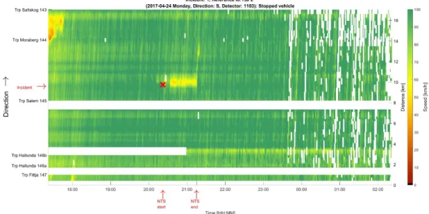
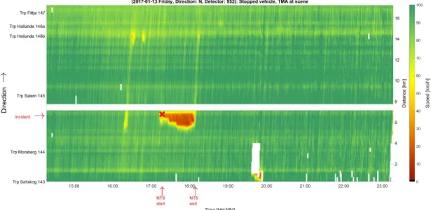
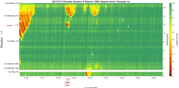
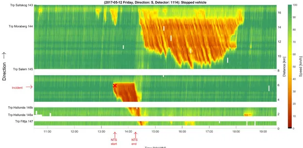
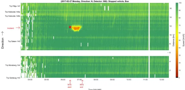
The 101 observations of stopped vehicle incidents were analyzed in detail during a one-day workshop with the project participants Ellen Grumert, Viktor Bernhardsson, Johan Olstam and Joakim Ekström. Figure 11 gives an example of the information provided for each incident. The figures present the time stamps for detection of an incident in NTS data and breakdown detections using the MCS data. The figures were used to classify if stationary traffic flow observations could be considered as observations of capacity or throughput. An observation of traffic flow at the incident site can be classified as the capacity if an incident has been detected (NTS start), but before a breakdown occurs (Last stationary before), while an observation of traffic flow at the incident site is classified as throughput after a breakdown has occurred (flow observations between First stationary after and NTS end). This approach was further elaborated for the subcategory stopped vehicle with one lane closure on homogenous road sections with the speed limit of 100 km/h. The output from the workshop were observations of capacity and throughput for the given subcategory, where uncertain observations of capacity and throughput were excluded. The identified observations were used for the estimation of capacity and the parameters of the fundamental diagram.
From the workshop it was concluded that even though the stopped vehicle incidents were categorized into similar subcategories based on number of closed lanes, speed limit and homogenous/off- or on-ramp location, the observed capacity might vary, probably due to circumstances and traffic conditions not observable in the available data, such as weather conditions, number of rescue units, lanes affected but not closed in MCS, etc.
Figure 11. Example of information provided for each incident at the workshop. The upper subplot illustrates the Variable Speed Limit sign status (recommended speed limit or closed lane ‘x’) and the lower sublot displays the stationary traffic conditions in terms of flow (blue line) and speed (red line), the NTS timestamps and the last stationary flow before traffic breakdown and first stationary flow after traffic breakdown.
3.3. Estimation of the capacity distribution
When observations of the capacity have been identified based on the approach described in section 3.2, the capacity can be estimated for the considered subcategory stopped vehicles at homogenous road sections with three lanes, one lane closed and a speed limit of 100 km/h. As concluded by Kondyli m.fl. (2017), the capacity is known to vary widely on a daily basis and even for similar traffic conditions and at the same site. Therefore, the capacity should be described and modelled as a
stochastic variable with a stochastic variable, rather than as a fixed value. The cumulative distribution function can be used to represent possible outcomes of the capacity (or the traffic flow at a
breakdown). To estimate the cumulative distribution function observations of capacity are required. The traffic flow observations classified as capacity observations in section 3.2. is used to estimate the cumulative distribution function. Different approaches exists in the literature and commonly suggested methods are the non-parametric product limit method (PLM) (Minderhoud m.fl., 1998) and the
parametric Maximum Likelihood Method (MLM) (Geistefeldt och Brilon, 2009, Minderhoud m.fl., 1997). A benefit with PLM is that it does not require a specific form of the cumulative distribution, however, the distribution function does only reach 1 if the observed maximum traffic flow is followed by a breakdown. MLM require a predefined form of the distribution function. In the literature a Weibull distribution is commonly assumed since it has been proven to give a good representation of the distribution of capacity in many previous empirical studies, see e.g. Minderhoud m.fl. (1997) or Geistefeldt och Brilon (2009). Besides the capacity observations, it is possible to make use of the observations of traffic flow before a breakdown since the capacity is known to be at least more than the observed traffic flow. However, during incidents the traffic conditions are changing due to for example a reduction in the number of available lanes and thereby this approach can only be used during normal traffic conditions. Instead, only the capacity observations are used to estimate the distribution of capacity. Since we only have observations resulting in breakdowns, the PLM will result in the full distribution function. Since MLM and PLM results in comparable distribution functions it is concluded that a Weibull distribution gives a good representation of the capacity distribution function also in this case. The resulting cumulative distribution functions using the two methods are shown in Figure 12 together with the expected value of the Weibull function.
Figure 12. The cumulative distribution function of capacity at stopped vehicle incidents at homogenous road sections with three lanes, one lane closed and a speed limit of 100 km/h.
As can be seen in Figure 12 there is a larger tail at lower flow levels. The reasons for this can probably be explained by the fact that not all explanatory variables have been identified due to limitations in the level of detail in the available incident data. For example, for very low-capacity observations it might be the case that more than one lane is indispensable, due to blocking of lanes by the stopped vehicle or the rescue units, etc., even though only one lane is closed according to the available MCS data. Other factors affecting the capacity can be weather or road conditions, the road design (curvature, slope,…), and etc. One question is also which value that is most correct to use in a traffic model, the expected value of the Weibull distribution or another probability level? One possibility is to illustrate the uncertainty in the estimate by using an upper and lower bound, such as for example the 95%- or 75%-percentile. However, the choice of upper and lower bound is related to how much of the extreme cases that should be covered and with a too wide range, such as the 95-% percentile, there is a risk to end up with a large number of possible outcomes. The effects the different percentiles will have on the resulting fundamental diagram is presented in section 3.4.
3.4. Estimation of the parameters of the fundamental diagram
The fundamental diagram is estimated for the subcategory stopped vehicles at homogenous road sections with three lanes, one lane closed and a speed limit of 100 km/h. The traffic flow observations classified as capacity and throughput, identified in the workshop described in section 3.2, is used to estimate the parameters of the uncongested and the congested part of the hyperbolic-linearfundamental diagram. Since some of the incidents occur at low traffic flows where the capacity never is reached, it should not be classified as throughput but rather the traffic flow corresponding to the current demand and related to the uncongested part of the fundamental diagram. Hence, a threshold related to the critical density is used to separate observations of traffic flow after the incident into traffic flow belonging to the uncongested part and throughput belonging to the congested part. The threshold value is based on the distribution of critical density, which is estimated similar to the capacity distribution in section 3.3. The distribution of critical density and the expected value used as threshold are shown in Figure 13. Only the traffic flow observations corresponding to a critical density value above the threshold value is categorized as throughput observations and used for the estimation of the congested part.
Figure 13. The cumulative distribution function of critical density for stopped vehicle incidents at homogenous road sections with three lanes, one lane closed and a speed limit of 100 km/h.
The congested and the uncongested part of the fundamental diagram is estimated by using MATLAB’s built-in function cftool, see MATLAB (2020a) for more details on the function. The optimization algorithm Levenberg-Marquardt is used to minimizes the absolute difference of the residuals (Least
0 50 100 150 200 Density (veh/km) 0 0.2 0.4 0.6 0.8 1 Probability (%) MLE estimation PLM estimation
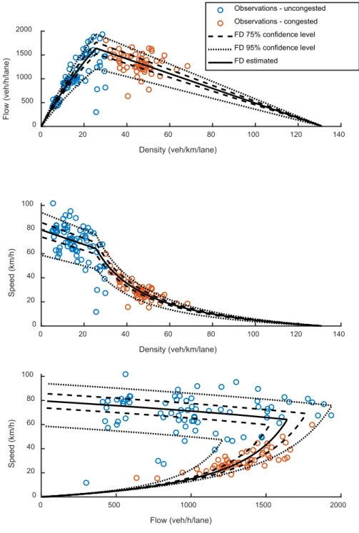
Absolute Residuals, LAR). The jam density is assumed to be identical to the case without an incident. All other parameters are estimated with the tool. The final fundamental diagram is given in Figure 14 and the resulting parameters are presented in Table 2. Two percentiles are presented to illustrate the uncertainties of the different percentiles. The fundamental diagram using the two percentiles have been adjusted by changing the capacity according to the percentiles in the capacity distribution and assuming that the critical density and the jam density is the same irrespective of percentile.
Table 2. Final parameters for the calibrated hyperbolic-linear fundamental diagram and upper and lower bounds using the 95%- and 75%-percentiles in the capacity distribution.
Parameter Estimated FD 95% percentile (low;high) 75% percentile (low;high)
𝐶𝐶 (veh/h/lane) 1640 (1210.5;1940.0) (1523.5;1768.5) 𝜌𝜌𝑚𝑚𝑚𝑚𝑚𝑚 (veh/km/lane) 131.5 (131.5;131.5) (131.5;131.5)
𝑉𝑉0 (km/h) 79.9 (58.8;94.2) (74.0;85.8)
𝜌𝜌𝑐𝑐𝑐𝑐𝑐𝑐𝑐𝑐(veh/km/lane) 51.2 (51.2;51.2) (51.2;51.2)
Figure 14. Calibrated hyperbolic-linear fundamental diagram with 75% and 95% percentiles. 0 20 40 60 80 100 120 140 Density (veh/km/lane) 0 500 1000 1500 2000 Flow (veh/h/lane) Observations - uncongested Observations - congested FD 75% confidence level FD 95% confidence level FD estimated 0 20 40 60 80 100 120 140 Density (veh/km/lane) 0 20 40 60 80 100 Speed (km/h) 0 500 1000 1500 2000 Flow (veh/h/lane) 0 20 40 60 80 100 Speed (km/h)
4.
Estimation of duration of incidents
An important aspect when estimating the effects of incidents is the incident duration, i.e. how much time elapses from the start of the incident to the incident site is cleared and the location of the incident is again unaffected in terms of capacity. During this time, the capacity per se may vary depending on the presence of rescue units (police, ambulance, fire service, etc.) and/or tow trucks. In order to get a rough idea of how the incident duration are influenced by different types of incidents, the extent of the incident and how many lanes that are blocked, disturbance reports from 468 incidents from Road Assistance (Vägvakt) have been compiled and analysed.
4.1. Data collection
To be able to estimate the duration of different types of incidents, a database was created from the disturbance reports from Vägvakt. The VägVakt reports includes more details about the incidents compared to the NTS reports, see chapter 2 for a description of the Vägvakt and NTS reports. Hence, the Vägvakt reports enables a more detailed analysis of how different potential explanatory variables might influence incident duration for different types of incidents. The database created based on the VägVakt reports contains the following information for each incident:
• Alarm time and end time for the incident
• Event type (accident, stopped vehicle, object and other phenomena)
• Blocking (left lane, middle lane, right lane, road shoulder and emergency pocket) • Number of vehicles and vehicle type and if rescue units were on site in the event of an
accident
• Reason for stopped vehicle (only relevant for incidents of event type stopped vehicle) • Type of object on the roadway (only relevant for incidents of event type object)
Out of the 468 disturbance reports from Vägvakt, 426 were of such quality that all information was included. Table 3 show the distribution of alarms with respect to incident type (accident, stopped vehicle or object) and number of blocked lanes or road shoulder and which lane that was blocked. Table 3. Distribution of alarms from the 426 disturbance reports that had complete information.
Accident Stopped vehicle Object
Total 50 301 75
1 lane blocked 19 153 29
2 lanes blocked 9 1 7
3 lanes blocked 0 0 1
Right lane + road
shoulder 4 21 2 Right lane 19 146 25 Middle lane 7 3 9 Left lane 24 6 12 Road shoulder 7 77 11
4.2. Analysis
The analysis has been done by calculating the mean value, standard deviation and confidence interval for different combinations of potential explanatory variables. Table 4 show the duration depending on the type of incident (accident, stopped vehicle or object) and the number of blocked lanes or road shoulder, including which lane that was blocked. 75%-confidence intervals were created to investigate if there is any statistically significant difference between incident duration for the different types of
incidents (accidents, stopped vehicles and objects on the roadway). On one hand, the analysis show that there is no statistically significant difference between accident and stopped vehicle incidents. On the other hand, there is a statistically significant difference between accident/stopped vehicle and objects on the roadway where the average value is approximately 52 minutes for accident/stopped vehicle and 26 minutes for objects on the roadway. The significance test between accident and stopped vehicle duration gives a result in the form - t-critical < t-Stat < t-critical gives a result of -1.16 < 0.47 < 1.16 (p-value = 0.64), between accident and object blockage duration in the form t-Stat > t-critical gives a result of 4.46 > 1.16 (p-value = 2.11664E-05) and between stopped vehicle and object
blockage duration in the form t-Stat > t-critical gives a result of 5.27 > 1:15 (p-value = 4.36396E-07). Table 4. Average duration and 75% confidence intervals (hours:minutes) divided by incident type and consequence based on blocked lane or road shoulder for the 426 disturbance reports with complete information.
Accident
duration Stopped vehicle duration Object blockage duration
1 lane blocked 00:43 ± 00:07 00:47 ± 00:03 00:22 ± 00:07 2 lanes blocked 01:09 ± 00:15 00:451) 00:22 ± 00:03
3 lanes blocked - - 01:15
Right lane + road shoulder
blocked 00:26 ± 00:05 00:57 ± 00:10 00:18 ± 00:32 Right lane blocked 00:46 ± 00:07 00:47 ± 00:03 00:27 ± 00:08 Middle lane blocked 01:09 ± 00:16 00:35 ± 00:20 00:29 ± 00:09 Left lane blocked 00:57 ± 00:08 00:46 ± 00:15 00:20 ± 00:06 Road shoulder blocked 00:59 ± 00:20 00:49 ± 00:05 00:12 ± 00:03
Mean value 00:53 00:51 00:26
Standard deviation 00:33 00:47 00:32
Confidence interval 75-% 00:05 00:03 00:04
Upper confidence value 00:58 00:54 00:31
Lower confidence value 00:48 00:48 00:22
1) Only one value, therefor have no confidence interval been calculated.
Table 5 show the incident duration for stopped vehicles considering the number of blocked lanes or road shoulder and the cause of the stopped vehicle. Results for accidents and objects on the roadway are presented in Appendix A. 75% confidence interval were created to investigate if there is any statistically significant difference between the incident duration when different number of lanes are blocked on the roadway at the incident site in the event of a stopped vehicle. The analysis shows no statistically significant difference at the 75 % confidence level between number of blocked lanes on the roadway. The significance test between 1 lane blocked and road shoulder blocked in the form - t-critical < t-Stat < t-t-critical gives a result of -1.15 < -0.34 < 1.15 (p-value = 0,73). Two blocked lanes is limited to one observation and three blocked lanes are never observed, why no t-tests can be
Table 5. Average duration and 75% confidence intervals (hours:minutes) in the event of a stopped vehicle divided by blocked lanes or road shoulder and reason for the stopped vehicle.
1 lane blocked 2 lanes blocked 3 lanes blocked Road shoulder
Engine etc. 00:48 ± 00:06 - - 00:54 ± 00:17 Towing 01:07 ± 00:10 - - 01:03 ± 00:21 Obstructive 00:57 ± 00:08 00:45 - 00:58 ± 00:11 Flat tire 00:43 ± 00:06 - - 00:47 ± 00:07 Out of gasoline 00:31 ± 00:09 - - 00:18 ± 00:04 Other reason 00:24 ± 00:25 - - 00:45 ± 00:14 Mean value 00:47 - - 00:49 Standard deviation 00:40 - - 00:42 Confidence interval 75-% 00:03 - - 00:05
Upper confidence value 00:51 - - 00:55
Lower confidence value 00:44 - - 00:44
Time of the day that the incident occur might influence the incident duration. To investigate if this is the case, the incidents were grouped based into four time intervals, irrespective of incident type, see Table 6. The result shows that there is a statistically significant difference for 1 blocked lane between 06:30-09:00 and the other time intervals during the day. Where the average value is 30 minutes for 06:30-09:00 and 41-52 minutes for the other time intervals. The significance test between 06:30-09:00 and 09:00-15:30 in the form t-Stat < t-critical gives a result of -2.91 < -1.16 (p-value = 0.005),
between 06:30-09:00 and 15:30-18:00 in the form t-Stat < t-critical gives a result of -2.19 < -1.16 (p-value = 0.031) and between 06:30-09:00 and 18:00-06:30 in the form t-Stat < t-critical gives a result of -1.82 < -1.16 (p-value = 0.073).
Table 6. Duration (hours:minutes) of all types of incidents divided into blocked lanes or roadside and time of day.
1 lane
blocked blocked 2 lanes blocked 3 lanes shoulder Road Total
06:30-09:00 Mean value 00:30 - - 00:48 00:43
Standard deviation 00:20 - - 00:29 00:45
Confidence interval 75-% 00:03 - - 00:17 00:06
Upper confidence value 00:34 - - 01:05 00:49
Lower confidence value 00:26 - - 00:30 00:36
15:30-18:00 Mean value 00:42 00:42 - 00:37 00:40
Standard deviation 00:35 00:25 - 00:37 00:35
Confidence interval 75-% 00:04 00:18 - 00:09 00:03 Upper confidence value 00:47 01:00 - 00:46 00:44 Lower confidence value 00:37 00:24 - 00:28 00:37
09:00-15:30 Mean value 00:52 00:47 - 01:02 00:56
Standard deviation 00:43 00:28 - 00:31 00:59
Confidence interval 75-% 00:07 00:20 - 00:13 00:07 Upper confidence value 00:59 01:07 - 01:16 01:04 Lower confidence value 00:44 00:27 - 00:48 00:48
18:00-06:30 Mean value 00:41 00:56 - 00:38 00:49
Standard deviation 00:36 00:46 - 00:35 00:43
Confidence interval 75-% 00:06 00:20 - 00:13 00:03 Upper confidence value 00:47 01:16 - 00:51 00:53 Lower confidence value 00:35 00:35 - 00:24 00:45
Table 7 show the results for stopped vehicles considering the possible impact of the time of the day on the incident duration. The analysis shows that there is no statistically significant difference with respect to the time of day at a 75% confidence level for stopped vehicle incidents. Hence, there is no need to differentiate the duration based on the time of the day for stopped vehicle incidents, which is useful knowledge when an estimate of the duration is required as an input in for example a scenario-based analysis or for travel-time prediction. Corresponding analysis (also showing no statistical difference) for accidents and objects on the roadway is available in Appendix A.
Table 7. Duration (hours:minutes) in the event of a stopped vehicle divided by number of blocked lanes or road shoulder and time of day.
1 lane
blocked blocked 2 lanes blocked 3 lanes shoulder Road Total
06:30-09:00 Mean value 00:43 - - 00:48 00:46
Standard deviation 00:49 - - 00:29 00:52
Confidence interval 75-% 00:10 - - 00:17 00:09
Upper confidence value 00:54 - - 01:05 00:55
Lower confidence value 00:32 - - 00:30 00:37
15:30-18:00 Mean value 00:43 - - 00:35 00:41
Standard deviation 00:36 - - 00:36 00:37
Confidence interval 75-% 00:05 - - 00:09 00:04
Upper confidence value 00:49 - - 00:44 00:46
Lower confidence value 00:37 - - 00:26 00:37
09:00-15:30 Mean value 00:55 - - 01:02 00:59
Standard deviation 00:39 - - 00:31 01:03
Confidence interval 75-% 00:07 - - 00:13 00:10
Upper confidence value 01:03 - - 01:16 01:10
Lower confidence value 00:47 - - 00:48 00:49
18:00-06:30 Mean value 00:49 - - 00:38 00:58
Standard deviation 00:37 - - 00:35 00:41
Confidence interval 75-% 00:07 - - 00:13 00:04
Upper confidence value 00:56 - - 00:51 01:02
Lower confidence value 00:42 - - 00:24 00:53
4.3. Summary of findings
The analysis shows that there is a statistically significant difference between the average duration of an accident or stopped vehicle and an object on the roadway, where the average value is approximately 50 minutes for an accident or stopped vehicle and 27 minutes for an object on the roadway.
The results show that there is a statistically significant difference between 1 blocked lane or road shoulder and 2 blocked lanes in the event of a stopped vehicle, where the average value is
approximately 44 minutes for 1 blocked lane or road shoulder and 1 hour and 2 minutes for 2 blocked lanes. The result also shows that there is a statistically significant difference between 1 blocked lane and 2 blocked lanes in the event of an accident where the average value is 43 minutes for 1 blocked lane and 1 hour and 20 minutes for 2 blocked lanes. Finally, the results show that there is a statistically significant difference between all blockages due to objects on the roadway. For 1 blocked lane the average is 17 minutes and for 2 blocked lanes the average is 23 minutes and for blocked roadside the average is 11 minutes.
Table 8. Average duration for the cases with statistically significant difference divided by incident type and blocked lanes or road shoulder.
1 lane
blocked blocked 2 lanes blocked 3 lanes shoulder Road Total
Accident 00:43 01:09 - 00:59 00:53
Stopped vehicle 00:47 - - 00:49 00:51
Object 00:22 00:22 - 00:12 00:26
The result of the analysis of duration at different times of the day shows that there is no significant difference between time of day regardless of how the data is divided.
Knowledge of incident duration and which aspects that might affect the incident duration is useful for Traffic Management Centers (as Trafik Stockholm). However, due to the large spread it might be an advantage to have a strategy where a start value is used in an initial estimation and then, if there are indications that the incident management will take longer time, the duration is adjusted to the average value and if indications of even longer incident management times the duration is adjusted to an upper confidence bound. Table 9 show possible start, average and upper bounds based on 75% confidence intervals of the duration data. If a strategy instead is based on 95% confidence intervals for the lower/start and upper bound, the strategy looks like in Table 10.
Table 9. Duration levels for duration estimation for incident traffic management purpose based on 75% confidence intervals.
Level blocked 1 lane blocked 2 lanes blocked 3 lanes shoulder Road Total
Accident Upper level 00:50 01:24 - 01:19 00:58 Average level 00:43 01:09 - 00:59 00:53 Start level 00:36 00:54 - 00:39 00:48 Stopped vehicle Upper level 00:50 - - 00:54 00:54 Average level 00:47 - - 00:49 00:51 Start level 00:44 - - 00:44 00:48 Object Upper level 00:29 00:25 - 00:15 00:31 Average level 00:22 00:22 - 00:12 00:26 Start level 00:15 00:19 - 00:09 00:22
Table 10. Duration levels for duration estimation for incident traffic management purpose based on 95% confidence intervals.
Level blocked 1 lane blocked 2 lanes blocked 3 lanes shoulder Road Total
Accident Upper level 00:55 01:38 - 01:37 01:02 Average level 00:43 01:09 - 00:59 00:53 Start level 00:31 00:40 - 00:21 00:44 Stopped vehicle Upper level 00:53 - - 00:58 00:56 Average level 00:47 - - 00:49 00:51 Start level 00:41 - - 00:40 00:46 Object Upper level 00:35 00:29 - 00:17 00:34 Average level 00:22 00:22 - 00:12 00:26 Start level 00:09 00:15 - 00:07 00:19