Co-Evolving Online High-Frequency Trading
Strategies Using Grammatical Evolution
Patrick Gabrielsson, Ulf Johansson and Rikard König
School of Business and Information TechnologyUniversity of Borås Borås, Sweden
{patrick.gabrielsson, ulf.johansson, rikard.konig}@hb.se Abstract—Numerous sophisticated algorithms exist for
discovering reoccurring patterns in financial time series. However, the most accurate techniques available produce opaque models, from which it is impossible to discern the rationale behind trading decisions. It is therefore desirable to sacrifice some degree of accuracy for transparency. One fairly recent evolutionary computational technology that creates transparent models, using a user-specified grammar, is grammatical evolution (GE). In this paper, we explore the possibility of evolving transparent entry- and exit trading strategies for the E-mini S&P 500 index futures market in a high-frequency trading environment using grammatical evolution. We compare the performance of models incorporating risk into their calculations with models that do not. Our empirical results suggest that profitable, risk-averse, transparent trading strategies for the E-mini S&P 500 can be obtained using grammatical evolution together with technical indicators.
I. INTRODUCTION
Since the introduction of electronic exchanges in the late 20th century, a number of sophisticated algorithms have been developed for discovering reoccurring patterns in financial time series. However, the most accurate techniques available produce opaque models, from which it is impossible to discern the rationale behind trading decisions. It is therefore desirable to sacrifice some degree of accuracy for transparency. One fairly recent evolutionary computational technology that creates transparent models, using a user-specified grammar, is grammatical evolution (GE) [1, pp. 9-24].
When developing trading models, it is necessary to consider both entry- and exit strategies. The entry strategy decides when to enter a bid or offer into the market (or when to remain idle), whereas the exit strategy decides when to cut losses short or when to take profit by closing open positions in the market. Furthermore, a highly desirable property of any trading model is a high return-to-risk ratio with a low trading cost. Therefore, a trading model needs to consistently produce positive returns whilst minimizing risk and trading costs.
The most lucrative form of trading is high-frequency trading, i.e. when trading decisions are made intra-day, usually using a minute-, second- or millisecond time resolution. In a high-frequency setting, the availability of timely, fundamental economic and financial information is scarce, hence technical indicators are employed in this study. Furthermore, the nature of high-frequency trading requires that information be
processed in real-time. Therefore, we employ a moving window to train, validate and test our trading strategies in order to create a method suitable for an online trading system.
The above discussion constitutes the rationale behind our study, i.e. to co-evolve profitable, high-frequency entry- and exit strategies using grammatical evolution, while minimizing risk and trading costs. The choice of using historical tick data from the E-mini S&P 500 index future market in our study is due to its high liquidity and because it is a leading indicator for US equity.
This paper is structured as follows. Chapter II introduces the theoretical framework on which this study is based with regards to financial market analysis and evolutionary method. Chapter III reviews related work. Chapter IV presents the methodology adopted in this paper, including the experimental approach used to evolve and validate our trading strategies. The results from the experiments are presented in Chapter V, followed by conclusive remarks and an elaboration on suggested future work in Chapter VI.
II. BACKGROUND A. Technical Analysis and Dow Theory
Using a high-level taxonomy, market analysis methods can be divided into fundamental analysis, technical analysis and quantitative analysis. Fundamental analysis involves a detailed study of the underlying economical-, financial- and political factors affecting the fair value of an asset, in order to determine if the actual market value of an asset is either undervalued or overvalued, hence creating an opportunity for investment. Quantitative analysis assumes markets are random, and hence, models the price-development of an asset as a stochastic process (a random walk), where investment opportunities are identified from the statistical properties of the financial time series. Technical analysis is based on the assumption that all available information is aggregated into the price of an asset and that there is a serial correlation between past-, current- and future prices. Therefore, technical analysis involves the study of historical price movements with the intention of forecasting future price movements.
Technical analysis has its roots in Dow Theory, developed by Charles Dow in the late 19th century and later refined and
published by William Hamilton in the first edition (1922) of his book “The Stock Market Barometer” [2]. Robert Rhea
developed the theory even further in “The Dow Theory” [3], first published in 1932. The six basic tenets of Dow Theory assume that; averages (prices) discount everything (i.e. the market reflects all available information), markets have three trends (a primary trend, a secondary trend and a minor trend), major trends have three phases (accumulation during the peak of a downtrend, public participation during a mature trend and distribution during the peak of an uptrend), averages must confirm each other (Dow required similar patterns in the Dow Jones Industrial Average and the Dow Jones Rails Average before a signal was confirmed), volume must confirm a trend (i.e. trading volume should increase in the direction of the major trend) and a trend is assumed to be in effect until it gives definite signals that it has reversed (a trend will maintain its momentum until an ambiguous signal verifies that a trend reversal is imminent).
Modern day technical analysis [4] is based on the tenets from Dow Theory, in which prices discount everything, price movements are not totally random and the only thing that matters is what the current price levels are. The reason why the prices are at their current levels is not important (in contrast to fundamental analysis). The basic method in technical analysis starts with an identification of the overall trend by using moving averages, peak/trough analysis and support and resistance lines. Once a trend has been identified, technical indicators are used to measure the momentum of the trend and the buying/selling pressure in the market. In the final step, the strength and maturity of the current trend, the reward-to-risk ratio of a new position and potential entry levels for new long or short positions are determined.
This paper adopts the theory underlying technical analysis, where technical indicators are used to discover price trends and to time market entry and exit.
B. Grammatical Evolution
Grammatical evolution (GE) [5], pioneered by Ryan, Collins and O'Neill, is an evolutionary algorithm which can be used to create computer programs in an arbitrary language. It draws its inspiration from genetics and evolution in the biological system. In the biological system, genetic information is stored as strings of nucleotides in DNA molecules. Each nucleotide triplet, called a codon, constitutes a code for a specific amino acid. In turn, sequences of amino acids form proteins, which are the building blocks for all life. The genetic code of an individual is called the individual's genotype, whereas the resulting set of proteins obtained through the expression of the genetic code is called the individual's phenotype. Proteins are created from the genetic code through the two processes of transcription and translation. Firstly, parts of the DNA string is transcribed into RNA molecules, in which codons are mapped onto anti-codons. An anti-codon contains the complement nucleotides found in DNA molecules. Once the DNA string has been transcribed into a RNA string, the string is traversed and each anti-codon triplet maps a sequence of amino acids. Finally, sequences of amino acids constitute the proteins which make up an individual (phenotype).
In GE, the DNA string is represented as a binary string, where eight consecutive bits represent a codon. The binary
string is then transcribed into an integer string, where each integer results from the mapping of the eight consecutive bits in the binary string. The integer string is then traversed, where each integer codes for a specific production rule. This is equivalent to the translation process in the biological system where a set of RNA anti-codons code for a sequence of amino acids, resulting in a protein. In GE, the sequence of rules make up a complete executable computer program [6, pp. 74-76].
In GE, the mapping process between the genotype (bit string) and the phenotype (computer program) is accomplished through a grammar definition. A grammar in GE is expressed in Backus-Naur (BNF) form, which is represented by the 4-tuple {N,T,P,S}, where N represents non-terminal elements and
T represents terminal elements of a programming language. P
represents production rules, which transform non-terminal elements into terminal elements. S is just a start symbol which itself is a non-terminal element [1, pp. 11-13]. For example, the simple grammar below has 7 production rules and consists of the following non-terminals N={<signal>, <forecast>, <var>,
<op>, <value>, <int>, <real>} and terminals T={snow, rain, humidity, temperature, 0, 0.5}:
<S> ::= if(<signal>) {<forecast>;} else {<forecast>;}
<signal> ::= <var> <op> <value> | (<signal>) and (<signal>)
<forecast> ::= snow | rain <var> ::= humidity | temperature <op> ::= < | >
<value> ::= <int> | <real> <int> ::= 0
<real> ::= 0.5
Following the mapping process from genotype to phenotype, assume the bit string has been transcribed to the following integer string:
23 5 8 12 33 7 1 14 15 17 6 9 16 5 1 2 3
The translation process works by scanning the grammar from left-to-right, top-to-bottom, looking for non-terminals. The integer string is also scanned from left-to-right, where each integer (codon) is decoded to decide how to turn terminals into terminals. In the above example, the first non-terminal is the start symbol <S>. When this non-non-terminal is encountered, the first integer (codon) in the integer string is read, i.e. the number 23. Since the non-terminal <S> only has one choice for its production rule, i.e. "if(<signal>)
{<forecast>;} else {<forecast>;}", the codon does not need to
be decoded, and hence the <S> symbol is replaced with the string "if(<signal>) {<forecast>;} else {<forecast>;}". The next non-terminal symbol is "<signal>" in the statement "if(<signal>)". The "<signal>" symbol's production rule, i.e. "<var> <op> <value> | (<signal>) and (<signal>)", has two choices, separated with the pipe "|" character. Therefore the next codon in the integer string needs to be decoded. A codon is decoded by taking the modulus of the integer codon value by the number of choices for the current production rule according to "c mod n" where c is the integer codon value and n is the number of choices for the current production rule. Since the integer codon value is 5 and the number of choices is 2 their
modulus yields the value "c mod n = 5 mod 2 = 1". If there are
n choices, each choice is numbered consecutively from 0 and
up to n-1. Therefore, the second choice is selected from the result of the modulus operation, i.e. "(<signal>) and
(<signal>)". This is then substituted into the original string in
place of the "<signal>" symbol in the "if(<signal>)" string, which yields the resulting string "if((<signal>) and
(<signal>)) {<forecast>;} else {<forecast>;}". This process is
repeated until all the non-terminals have been replaced by terminals.
Selection, crossover and mutation on the bit string (genotype) is handled in the same way as in the traditional genetic algorithm (GA). Likewise, the population size and the number of generations are used to control the evolutionary process as in the genetic algorithm.
Since grammatical evolution (GE) produces transparent models, it was selected as the evolutionary strategy for our study. Version 2.0 of the freely available GE software GEVA (Grammatical Evolution in jaVA) [7] was used to evolve our trading models. A comprehensive list of research relating to GE can be found in [8].
III. RELATED WORK
In [6, pp. 183-192], Grammatical Evolution (GE) was used to create trading models for the daily prices of the indices FTSE, Nikkei and DAX. Two technical indicators, moving average and momentum, were used. The induced models produced buy and sell signals for market entry, using a fixed horizon for the exit strategy. The fitness function used for the GE, included the average return and the maximum drawdown in its calculations. The produced models outperformed their benchmark, based on a buy and hold strategy. The study showed that, by incorporating risk (maximum drawdown), into the fitness function, less riskier models were obtained, as compared to the benchmark strategy.
In [6, pp. 193-201], a similar study was conducted, where a moving window was used to retrain the model every 5 trading days. During training, information from the newly added 5 days of market data were used, together with the model's previous data, to adapt the model to prevailing market conditions. Only a single technical indicator, moving average, was included as a component in the GE grammar, but the size of each trade was based on the strength of the trading signal produced by then model. In this study, the fitness function was based on the model's total return and did not include any trading costs. The adaptive model was benchmarked against a static model (no memory), in which the static model was completely retrained every 5 trading days. The results imply that an adaptive model performs better than a static model.
In [6, pp. 203-210], intra-day trading models were created with GE. Three models, each using a different exit strategy, were benchmarked against each other. The first model closed a position after 30 minutes, whereas the second model extended the open position for another 30 minutes if the model's prediction was still valid. The third model used an exit strategy based on a 0.1% stop-loss and a 0.8% take-profit. The fitness function used for all three models did not include any risk or trading costs in its calculations. The study showed that the exit
strategy based on a stop-loss/take-profit, outperformed the other two strategies. In turn, the extended close strategy outperformed the standard close strategy.
In [9] and [10], the entry- and exit strategies were coevolved using GE. In [9], the fitness function incorporated risk and trading costs into its calculations, where the standard deviation of the total return was used as a proxy for risk. In [10], four different fitness functions were benchmarked against each other, although trading costs were not included in the calculations. Both studies showed clear benefits of coevolving entry- and exit strategies with regards to profitability.
This study combines the approaches used above to co-evolve profitable, high-frequency entry- and exit strategies using grammatical evolution, while minimizing risk and trading costs. A moving window is used to retrain the models after each fourth trading day on minute data. Three different trading models are benchmarked against each other. The first model's fitness function incorporates trading costs and risk, based on the maximum drawdown, in its calculations. The second model's fitness function incorporates trading costs, but does not consider risk. The third model is based on a random trading strategy. This combination constitutes the novelty in the study.
IV. METHOD A. Data Acquisition and Feature Extraction
The S&P (Standard and Poor’s) 500 E-mini index futures contract (ES), traded on the Chicago Mercantile Exchange, was chosen for the research work. Two months worth (5th July – 2nd
September 2011) of tick data was downloaded from Slickcharts [11] which provides free historical intra-day data for E-mini contracts.
A tick is the minimum amount a price can be incremented or decremented for a certain contract. For the E-mini S&P 500, the minimum tick size is 0.25 points, where each tick is worth $12.50 per tick and contract.
The data was aggregated into one-minute bars, each including the open-, high-, low- and close prices, together with the 1-minute trade volume. Missing data points, i.e. missing tick data for one or more minutes, was handled by using the same price levels as the previously existing aggregated data point.
Two technical indicators were chosen in order to extract trend and momentum information from the aggregated data; the simple moving average indicator and the relative strength indicator [4]. The parameter values for these indicators were optimized by the grammatical evolution process.
B. Dataset Partitioning
The dataset was split into ten folds, each of size k=5610 data points (5610 minute bars), equivalent to 4 trading days, in order to support a validate-test" (i.e. an online "train-backtest-trade") approach. This was accomplished by creating a large enough window of size N=22440 data points (4 folds = 16 trading days), to be used as the initial training set. The trading model was then trained using the training window, validated (backtested) on the closest two folds preceding the
training window and tested (traded) on the closest fold succeeding the training window. Following this, the training
window was rolled forward one fold (4 trading days) and the train-validate-test procedure was repeated. In total, four training windows were used over the chosen dataset. The training, validation and test datasets are shown in Fig.1. The initial training window (training window 1) is show in the middle of the figure, bounded by a black box, preceded by its two validation folds and succeeded by its single test fold. The range of training windows 1-4 are shown along the bottom of the figure.
C. Fitness Function and Performance Measures
A fitness function can be based on simple returns, calculated according to (1), where Pt-1 denotes the price of the asset when the position is opened, Pt denotes the price of the asset when the position is closed and is equal to 1 if the asset was bought when the position was opened or equal to -1 if the asset was short-sold.
The problem with such a fitness function is its inability to incorporate risk into its calculation. Therefore, one commonly used measure of a trading strategy's fitness is the Sharp Ratio [6, pp. 124]. The Sharp Ratio determines the rate of a model's average return (adjusted for the risk-free rate) and its standard deviation according to (2) where (3) is the average return and (4) is the standard deviation of the return.
The risk-free rate (federal funds) is only applicable if a trade is carried over night (from one trading day to another), which is not the case in high-frequency trading where all open
positions are closed before the end of the trading day. Therefore, the Sharp Ratio for high-frequency trading is calculated according to (5).
However, the Sharp Ratio only gives an accurate measure if the returns are normally distributed. This is due to (4) and is easily seen by observing that both positive and negative deviations from the average return are incorporated in its calculation. Hence, the Sharp Ratio summarizes the average deviation from the average return and does not account for the risk of extreme negative effects that can be detrimental to profits. Therefore, a better risk-adjusted measure is the Calmar Ratio (6), which uses the maximum drawdown (MD) as its risk measure [6, pp. 124]. The maximum drawdown measures the largest drop in returns during a trading period which is a better measure of risk as compared to the standard deviation.
Once again, the risk-free rate is only applicable if a trade is carried over night. Therefore, the Calmar Ratio for high-frequency trading is calculated according to (7).
Finally, trading costs need to be incorporated in the fitness function. Trading costs consist of commission fees, transaction fees, brokerage fees, interest fees, tax fees and slippage in the form of market impact, liquidity and other unforeseen circumstances causing a discrepancy between the estimated- and actual trading costs. Interest fees (risk free rate) are not applicable in high-frequency trading and can therefore be omitted. This study does not consider taxes on returns or slippage due to market impact and liquidity (liquidity issues are reduced since we only trade one-lots), hence the effects of larger, dynamically sized market orders are not assessed. This leaves us with commission fees, transaction fees and brokerage fees. These fees are highly dependent on which brokerage is
used, exchange membership and other circumstantial factors. Nevertheless, fees of 20%-30% on returns are reasonable estimates. Therefore, we will incorporate an approximate trading cost in our performance measure by deducting $3 per roundtrip, i.e. every time we close an open position, we will deduct $3 from the return regardless if the return is positive or negative. Our resulting fitness function is calculated according to (8), i.e. as the average cost-adjusted return divided by the maximum drawdown, where the maximum drawdown is based on the cumulative cost-adjusted returns.
In order to evaluate the performance of the trading models obtained by using a risk-adjusted fitness function, we benchmark them against models obtained using a fitness function based solely on return (9).
Numerous performance measures are used to evaluate the performance of a single trading model and to compare performances of multiple trading models [6, pp. 137-140]. The most common measures have already been described, i.e. the return, mean and standard deviation of the return, Sharp ratio and maximum drawdown. Furthermore, it is of interest to know the number of trades produced by a trading model, the trade frequency (i.e. trades per trading day) and the average time a trade remains in the market. These last three measures are all proxies for risk. Besides these single-number performance measures, equity curves are used to visualize the continuous performance and risk associated with the trading models. We include all the above performance measures and equity curves in our analysis.
D. Experiments
The grammar for the grammatical evolution of the entry- and exit strategies was defined as below. Here we permit any combination of technical indicators and values. We include "domain" knowledge in the form of our if-statements, i.e. we know we need a ternary decision for the entry strategy (buy, sell or remain idle) and for the exit strategy (exitlong, exitshort and remain idle) [9].
<enterrule> ::= if(<signal>) {<trade>;} else {<trade>;}
| if(<signal>) {<trade>;} else if {<signal>} {<trade>;} else {<trade>;}
<trade> ::= buy(i) | sell(i) | idle() <signal> ::= <var> <relop> <var> | <var> <relop> <value> | (<signal>) "&&" (<signal>) | (<signal>) "||" (<signal>) <var> ::= px(i) | sma(i,<int>) | rsi(i,<int>) <relop> ::= "<=" | ">=" | "==" | "<" | ">" <value> ::= <int> | <real> | <int><real> <int> ::= <GECodonValue(1,300)>
<real> ::= .1|.2|.3|.4|.5|.6|.7|.8|.9
<exitrule> ::= if(<signal>) {<exit>;} else {<exit>;} | if(<signal>) {<exit>;} else if {<signal>}
{<exit>;} else {<exit>;}
<exit> ::= exitlong() | exitshort() | idle() <signal> ::= <var> <relop> <var>
| <var> <relop> <value> | (<signal>) "&&" (<signal>) | (<signal>) "||" (<signal>) <var> ::= px(i) | sma(i,<int>) | rsi(i,<int>) <relop> ::= "<=" | ">=" | "==" | "<" | ">" <value> ::= <int> | <real> | <int><real> <int> ::= <GECodonValue(1,300)>
<real> ::= .1|.2|.3|.4|.5|.6|.7|.8|.9
The parameters for the grammatical evolution were set according to Table I.
Different GE parameter settings were experimented with, before arriving at the settings presented in Table I, such as various combinations of population sizes, selection operators, crossover schemes and elitism sizes. Especially, it was found that using a higher mutation rate destroyed heritability and increasing the number of generations beyond 50 did not severely affect the convergence of the population. Steady state replacement was not considered, although it is hypothesized that this could be beneficial for a continuous adaption of the trading strategy to changing market conditions.
The evolutionary procedure commenced as follows. Initially, 1000 individuals were randomly created to populate the first generation and each individual's genotype was mapped to its phenotype by decoding the individual's codons using the grammar. Each individual was then evaluated on the training set using the fitness function. The individuals in the current generation were then used to populate the next generation using tournament selection, crossover and mutation. Since a generational replacement strategy was used, the entire current generation was replaced by the next generation (as opposed to the steady state approach used in [6, pp. 193-201]). Additionally, the fittest individual in the current generation was copied, unaltered, to the next generation. The fitness evaluation, selection, crossover, mutation and replacement process was then repeated for a total of 50 generations. The fittest individual in the final generation was then chosen as the winner and its phenotypic strategies were back tested and evaluated on the validation dataset.
TABLEI GEPARAMETERS
Parameter Setting
Generations 50
Population Size 1000
Selection Operator Tournament Selection
Tournament Size 3
Crossover Operator Single Point Crossover Crossover Probability 0.8
Mutation Operator Bit Flip Mutation Probability 0.01
Replacement Type Generational
Elitism True
This process was repeated 30 times in order to calculate an average performance measure on the validation dataset, since the results produced by GE are non-deterministic. Furthermore, the individual with the highest performance measure on the validation dataset was chosen as the optimal trading strategy for the test dataset. Although, to yield an average performance measure on the test dataset (for comparison purposes), all 30 individuals from the validation set were evaluated on the test set.
The training window was then rolled forward and the process above was repeated. This was done for all four training windows. Finally, the results were examined, together with the trading strategies for all datasets.
The above procedure was carried-out for both the risk-adjusted fitness function and the fitness function based solely on return. Furthermore, the procedure was repeated for a random trading strategy. The random trading strategy randomly selected an entry decision from the set {buy, sell, idle} every minute. The exit strategy was time-based, i.e. each order was kept in the market a random amount of minutes, from the range [0,100], followed by closing the position.
V. RESULTS
The performance measures for the risk-adjusted fitness function are tabulated in Table II. The table displays the various measures for each window (1-4), each consisting of a training-, validation- and test dataset. All measures are averages of 30 runs. There is also a total average given over all datasets at the bottom of the table. The first column displays the dataset, followed by the total return in the second column. The remaining columns show the Sharp Ratio (SR), Maximum Drawdown (MD), Trade Count (TC), Trade Frequency (TF) and Time In Market (TIM) respectively. The trade frequency is based on trades per day and the time in market is expressed in minutes.
By inspecting Table II, it is obvious that all average returns are positive. Furthermore, the mean and standard deviation of the returns reveal that most individual trades yielded positive returns. The Sharp Ratio is above 2 in all but two data sets (window 3), which indicates a relatively low risk investment (values above 2 are indicative of a good return-to-risk ratio). Besides the validation- and test datasets in window 3, the maximum drawdown is virtually negligible. The trade count and trade frequency is kept at a minimum by the risk-averse objective function. The time in the market varies from dataset to dataset yielding relatively large values in one validation dataset (window 1) and one test dataset (window 3). The total average over all datasets, shows that the risk-adjusted fitness function produced profitable trading strategies across all datasets with relatively high average returns and low dispersions (good Sharp Ratio). The trade frequency was relatively low and no substantial sudden drops in returns (maximum drawdown) were recorded during trading. Therefore, as hypothesized, the fitness function has produced profitable, risk-averse trading strategies.
The performance measures for the fitness function based solely on return are tabulated in Table III.
The results presented in Table III show that the fitness function, based solely on return, yields positive average returns in all but two test datasets (in window 1 and 4). Noticeably, the returns have relatively low means and high standard deviations. This produces low Sharp Ratios and therefore risky investments, which is also confirmed by the substantial draw-downs. The trade counts and trade frequencies are also high. On average, the time an order is in the market before it is closed lies between 16-68 minutes. Compared to the risk-adjusted fitness function, the fitness function based solely on the return produces much higher returns, on average, whilst taking on much higher risk (draw-downs). This confirms the
TABLEIII
Performance Results (Return-Only Fitness Function)
Dataset Return ($) SR MD TC TF TIM
WINDOW 1 Train 663,477 0.18 -220,176 20077 1254 74.23 Valid 220,720 0.22 -51130 9993 1249 72.15 Test -33,517 -0.02 -244264 5017 1254 87.93 WINDOW 2 Train 721,852 0.17 -243995 19888 1242 65.75 Valid 143,972 0.07 -220008 15370 1921 90.95 Test 90,727 0.13 -72281 4727 1181 56.92 WINDOW 3 Train 728,823 0.17 -242237 19207 1200 66.28 Valid 14,990 0.01 -218548 9949 1243 88.65 Test 317,502 0.43 -35126 4711 1177 60.49 WINDOW 4 Train 917,570 0.20 -242469 19613 1225 62.75 Valid 199,594 0.21 -72918 9970 1246 64.36 Test -99,742 -0,09 -260013 5148 1286 117.91 TOTAL AVERAGE Train 757,931 0.18 -237219 19697 1231 67.25 Valid 144,819 0.13 -140651 11321 1415 79.03 Test 68,742 0.11 -152921 4901 1225 16.24 TABLEII
Performance Results (Risk-Adjusted Fitness Function)
Dataset Return ($) SR MD TC TF TIM
WINDOW 1 Training 19,596 2.28 -0.52 44 2.76 59.91 Validation 17 2.21 -3.47 12 1.54 330.10 Test 113 2.05 -1.77 3 2.25 11.10 WINDOW 2 Training 20,937 2.16 -0.50 51 3.18 61.24 Validation 85 2.37 -0.50 4 0.50 12.00 Test 957 122.4 -0.15 3 0.77 46.74 WINDOW 3 Training 21,166 2.29 -0.50 47 2.91 56.55 Validation 3 0.00 -6.50 22 2.75 0.36 Test 65 0.69 -35.28 6 1.57 135.52 WINDOW 4 Training 21,104 2.38 -0.40 41 2.58 62.82 Validation 27 2.26 0.00 6 0.75 11.17 Test 2,568 4,49 -32.22 7 1.75 51.83 TOTAL AVERAGE Training 20,701 2.28 -0.48 46 2.85 60.13 Validation 33 1.71 -2.62 11 1.39 88.41 Test 926 41.71 -17.35 5 1.58 61.30
hypothesis that, using a risk-adjusted fitness function, produces more reliable investments. Although, on this particular set of datasets, the return-only fitness function creates substantially more wealth, on average.
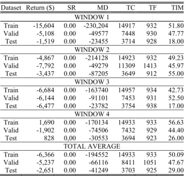
Finally, Table IV shows the results obtained using the random strategy.
Except for the training- and test datasets on window 4, the random trading strategy produced negative returns on all datasets. The results show that the average return on all datasets is close to zero with a high standard deviation, which is expected from a random strategy. As a consequence, the Sharp Ratio is close to zero and the maximum drawdown is substantial. The trade count and trade frequency is also relatively high. The time an order is spent in the market is unimportant, since this was randomly chosen by the random trading strategy.
The results for all three strategies are visualized as equity curves, on all datasets, in Fig. 2. The best results of all
strategies on all datasets are tabulated in Table V. As can be seen in Fig. 2, the strategies acquired using the risk-adjusted fitness function, produce (almost) non-decreasing equity curves. Hence, these strategies are profitable and risk-averse. Compared to the return-only fitness function, the number of trades are considerably smaller for the risk-adjusted strategy.
For the return-only equity curve, the GE algorithm still managed to find profitable trading strategies, albeit with a considerably larger amount of risk. The performance is relatively good on the validation set, with upward-trending equity curves in all windows. The average profits are also good on the test datasets, although the substantial drawdown is noticeable.
As expected, the random strategy yields a highly stochastic behavior with substantial draw-down on most datasets. This compares to the performance of the zero-intelligence strategy used in [9].
TABLEV
Performance Results (Best individuals in each dataset)
Dataset Return ($) SR MD TC TF TIM
TEST WINDOW 1 RiskAdj 87.0 87.0 0.00 1 0.25 4.00 Return -2.730.50 0.00 -239339.50 5536 1384.00 77.97 Random -1,519.50 -0.00 -23455.50 3714 928.50 18.00 TEST WINDOW 2 RiskAdj 1,934.00 1.65 -0.50 7 1.75 48.29 Return 75860.00 0.07 -90408.00 5505 1376.25 44.52 Random -3,437.00 -0.00 -87205.50 3649 912.25 55.00 TEST WINDOW 3 RiskAdj 444.00 0.47 -77.50 12 3.00 37.50 Return 282308.00 0.50 -34345.50 3009 752.25 85.78 Random -6,477.00 -0.01 -23782.50 3754 938.50 17.00 TEST WINDOW 4 RiskAdj 1,634.00 0,88 -25.50 7 1.75 31.71 Return -78,907.50 -0.07 -228615.50 5190 1297.50 100.44 Random 828.00 0.00 -30553.00 3694 923.50 26.00 TOTAL AVERAGE RiskAdj 1,024.75 29.71 -25.87 7 1.69 30.37 Return 93,086.83 0.13 -148177.13 4810 1202.50 77.18 Random -2,651.37 0.00 -41249.13 3703 925.69 29.00 TABLEIV
Performance Results (Random Trading Strategy)
Dataset Return ($) SR MD TC TF TIM
WINDOW 1 Train -15,604 0.00 -230,204 14917 932 51.80 Valid -5,108 0.00 -49577 7448 930 47.77 Test -1,519 0.00 -23455 3714 928 18.00 WINDOW 2 Train -4,867 0.00 -214128 14923 932 49.23 Valid -7,792 0.00 -49279 11309 1413 45.97 Test -3,437 0.00 -87205 3649 912 55.00 WINDOW 3 Train -6,684 0.00 -163740 14957 934 42.73 Valid -6,144 0.00 -91101 7453 931 52.50 Test -6,477 0.00 -23782 3754 938 17.00 WINDOW 4 Train 1,690 0.00 -170134 14933 933 56.63 Valid -1,902 0.00 -74506 7432 929 44.40 Test 828 0,00 -30553 3694 923 26.00 TOTAL AVERAGE Train -6,366 0.00 -194552 14933 933 50.09 Valid -5,237 0.00 -66116 8411 1051 47.67 Test -2,651 0.00 -41249 3703 925 29.00
From the equity curves, the hypothesis that the GE managed to find profitable trading strategies in the provided search space holds. This fact is confirmed by the observable difference between the random strategy and the other two strategies.
One specific profitable entry strategy obtained from the grammatical evolution is shown below. The first rule constitutes the entry strategy which is easily interpreted as "if the price is over its 100-period SMA and the 5-period RSI is below 15 then buy, else if the price is under its 150-period SMA and the 10-period RSI is above 80 then sell, otherwise do nothing". In other words, if the index is trending upwards and is considered oversold, then buy. Conversely, if the index is trending downwards and the index is considered overbought, then sell.
if( ( px(i) > sma(i,100) ) && ( rsi(i,5) < 15 ) ) {buy(i);}else if( ( px(i) < sma(i,150) ) && ( rsi(i,10) > 80 ) ) {sell(i);} else {idle(i);}
VI. CONCLUSIONS AND FUTURE WORK
In this study we hypothesized that profitable trading strategies (entry and exit) could be coevolved for the E-mini S&P 500 using grammatical evolution (GE) together with technical indicators (SMA and RSI). We further hypothesized that the obtained trading strategies were based on patterns discovered in the historical prices and not simply caused by chance. This was confirmed by benchmarking the results with a random trading strategy. We compared the trading strategies obtained from a risk-adjusted fitness function and a return-only fitness function. The results suggest that risk-averse trading strategies can be obtained by incorporating risk together with return into an objective fitness function. Although, the return-only fitness function yielded substantially higher returns on average, it took on considerably more risk than the risk-averse fitness function. The GE algorithm produced transparent, comprehensible models and the obtained trading rules were easily deciphered.
In this study, we only considered two technical indicators as components in the grammar for the GE. It would be interesting to incorporate more indicators into a future study. Furthermore, we only considered the E-mini S&P 500 index future market. There are a plentitude of other markets that can
be considered in a future study, including other asset classes and cross-market trading strategies.
The study did not consider the effects of larger, dynamically sized market orders (or unfilled limit orders) with respect to market impact. For practical purposes, this needs to be incorporated into a future study.
The GE framework provides an excellent opportunity to incorporate domain-specific knowledge into the search process through its grammar. This enables the possibility of evolving more targeted trading strategies. The GE framework's pluggable architecture also permits a future experimentation with various search strategies, besides the canonical form of GA used in this study, such as island-based GA or swarm-based search methods.
Finally, it is expected that better results can be obtained in a future study by using larger datasets and by exploring other fitness functions.
REFERENCES
[1] I. Dempsey, M. O'Neill and A. Brabazon, Foundations in Grammatical
Evolution for Dynamic Environments, 1st ed. Springer-Verlag, 2009.
[2] W. P. Hamilton, The Stock Market Barometer: Wiley, 1998. [3] R. Rhea, The Dow Theory: Fraser Publishing, 1994.
[4] J. Murphy, Technical Analysis of the Financial Markets: New York Institute of Finance, 1999.
[5] C. Ryan, J.Collins and M.O'Neill, Grammatical Evolution: Evolving
programs for an arbitrary language. In: W. Banzhaf, R. Poli, M.
Schoenauer, et al., eds. Proc of the First European Workshop on Genetic Programming (EuroGP98), LNCS, 1998, 1391: p 83–96.
[6] A. Brabazon and M. O'Neill, Biologically Inspired Algorithms for
Financial Modelling, 1st ed. Springer-Verlag, 2006.
[7] GEVA, 2013. [Online]. Available: http://ncra.ucd.ie/Site/GEVA.html. [Accessed: 20-Apr-2013].
[8] Grammatical Evolution, 2013. [Online]. Available: http://www.grammatical-evolution.com/pubs.html. [Accessed: 20-Apr-2013].
[9] R. Bradley, A. Brabazon, and M. O’Neill, Evolving Trading Rule-Based
Policies, in Applications of Evolutionary Computation, C. Chio, et al.,
Editors. 2010, Springer Berlin Heidelberg. p. 251-260.
[10] K. Adamu and S. Phelps, Coevolutionary Grammatical Evolution for
Building Trading Algorithms, in Electrical Engineering and Applied Computing, S.-I. Ao and L. Gelman, Editors. 2011, Springer
Netherlands. p. 311-322.