Terence McGarvey
Barrier separated road type design
Accelerated degradation
VTI r apport 925A | Barrier separ ated road type design. Acceler
www.vti.se/en/publications
VTI rapport 925A
Published 2017
VTI rapport 925A
Barrier separated road type design
Accelerated degradation
Abstract
To reduce the risk of vehicular head-on collisions, the Swedish Transport Administration
(Trafikverket), has been transforming high traffic-volume conventional roads into barrier separated roads. This process has reduced the number of fatalities by around 80 percent.
However, evidence has shown that barrier separated roads degrade quicker than conventional road types.
The extent of the problem was quantified by comparing various sets of road surface characteristic data. Comparisons revealed that degradation levels increase by up to 60 percent in the single lane sections of 2+1 type barrier separated roads.
Vehicle position surveys were carried out and subsequent data analysis confirmed that confinement of vehicle lateral wander is a main cause of the problem. The analysis indicated that in the single lane section of a 2+1 type barrier separated road, vehicle lateral wander reduced by 24 percent for light vehicles and 19 percent for commercial traffic. These figures increased to 44 percent and 39 percent for a 1+1 type barrier separated road.
Accelerated degradation can be attributed to poor cross-sectional design. The amount of vehicular lateral wander is restricted and results in surface wear and loading being concentrated in narrow tracks along the road section.
Design improvements are possible but will obviously require higher initial investment expenditure.
Title: Barrier separated road type design - accelerated degradation
Author: Terence McGarvey
Publisher: Swedish National Road and Transport Research Institute (VTI)
www.vti.se
Publication No.: VTI rapport 925A
Published: 2017
Reg. No., VTI: 2006/0011-290
ISSN: 0347-6030
Project: 2+1 Väg och breddning av väg
Commissioned by: Swedish Transport Administration
Keywords: 2+1, barrier separated road, lateral wander, degradation
Language: English
Referat
För att minska risken för frontalkrockar har Trafikverket omvandlat högt trafikerade traditionellt utformade vägar till mötesfria vägar. Denna omvandlingsprocess har minskat antalet dödsolyckor med ungefär 80 procent.
Dock har det visat sig att mötesfria vägar bryts ner snabbare än traditionellt utformade vägar. Omfattningen av problemet har kvantifierats genom att jämföra olika datauppsättningar om vägytors karakteristiska egenskaper. Dessa jämförelser visade att spårdjupsutvecklingen ökade upp till 60 procent på de enfiliga sträckorna av mötesfria vägar som 2+1-vägar.
Undersökningar av fordonsposition utfördes också och en efterföljande analys bekräftade att inskränkning i fordonens sidolägesvariation utgjorde en väsentlig del av problemet. Analysen
indikerade att på enfiliga sträckor av 2+1-vägar minskade sidoförflyttning med 24 procent bland lätta motorfordon och 19 procent bland tunga. Dessa siffor ökade till 44 procent respektive 39 procent för 1+1-vägar.
Accelererad nedbrytning uppstår på grund av dålig tvärsnittsdesign. Sidoförflyttning av fordon begränsas, vilket resulterar i slitage och att belastning koncentreras till smala spår längs med vägsträckan.
Designförbättringar är möjliga, men kräver större initiala investeringsinsatser.
Titel: Mötesfria vägar – accelererad nedbrytning
Författare: Terence McGarvey
Utgivare: VTI, Statens väg- och transportforskningsinstitut
www.vti.se
Serie och nr: VTI rapport 925A
Utgivningsår: 2017
VTI:s diarienr: 2006/0011-290
ISSN: 0347-6030
Projektnamn: 2+1 Väg och breddning av väg
Uppdragsgivare: Trafikverket
Nyckelord: 2+1, mötesfria vägar, sidolägesvariation, accelererad nedbrytning
Språk: Engelska
Foreword
This project has been funded in total by the Swedish Transport Administration.
Investigations, data analysis, photographing and report writing have been carried out by Terence McGarvey (VTI).
Thanks, are given to Håkan Wilhelmsson (VTI) and Sven-Åke Lindén (formerly of VTI) who carried out the vehicle position surveys, and to Thomas Lundberg (VTI) who provided support regarding road surface survey data.
Final thanks are extended to Nils-Gunnar Göransson (VTI) and Carl-Gösta Enocksson (Swedish Transport Administration) for support and advice given throughout the project duration.
Linköping, June 2017
Terence McGarvey Project leader
Process for quality review
Internal peer review was performed on 11 May 2016 by Anna Arvidsson. Terence McGarvey has made alterations to the final manuscript of the report. The research director Anita Ihs has examined and approved the report for publication on 21 March 2017. The conclusions and recommendations expressed are the author’s and do not necessarily reflect VTI’s opinion as an authority.
Process för kvalitetsgranskning
Intern peer review har genomförts 11 maj 2016 av Anna Arvidsson. Terence McGarvey har genomfört justeringar av slutligt rapportmanus. Forskningschef Anita Ihs har därefter granskat och godkänt publikationen för publicering 21 mars 2017. De slutsatser och rekommendationer som uttrycks är författarens egna och speglar inte nödvändigtvis myndigheten VTI:s uppfattning.
Contents
1. Introduction ...13 2. Aim ...14 3. Method ...15 4. Accelerated Degradation ...16 General ...16 Evidence ...16 Example Studies ...17 Conclusion ...235. Possible causes of accelerated degradation ...24
6. Confinement of vehicle lateral wander ...25
General ...25
Vehicle position surveys ...25
Conclusion ...30
7. Unsuitable surfacing ...31
Specification...31
Conclusion ...31
8. Vehicle speed increase ...32
Average speeds ...32 Surface Wear ...32 Commercial Vehicles ...33 Conclusion ...33 9. Design ...34 Design guidelines ...34 Longitudinal alignment ...34 10. Construction ...36 Road widening ...36 Transition Points ...37
Interface between new and existing construction ...40
11. Vehicle Position ...41
Plotting vehicle position ...41
Surveyed average positions and standard deviations ...42
Wide side-verge example ...46
Cross section design improvements ...47
Reductions in recommended design widths ...52
Conclusion ...53
12. Update of VTI Surface Wear Model...54
13. Recommendations and further research ...55
Design – Conversion of 9 m road to 2+1 ...55
Vertical construction joints ...57
VTI Surface wear model ...57
Construction standards ...57 Referenser ...59 Appendix 1 ...61 Appendix 2 ...63 Appendix 3 ...65 Appendix 4 ...73 Appendix 5 ...75 Appendix 6 ...77 Appendix 7 ...79 Appendix 8 ...81
Summary
Barrier separated road design (2+1) – Accelerated degradation by Terence McGarvey (VTI)
Barrier separated roads enable near-motorway safety levels to be achieved at a much lower cost than with actual conversions to motorway or dual carriageway standards. Transforming a high traffic volume road into a barrier separated road type reduces the number of fatalities by around 80 percent. A large percentage of the high traffic volume road network in Sweden has already been transformed into 2+1 roads.
However, evidence has shown that barrier separated roads degrade quicker than conventional road designs.
The extent of the problem was quantified by comparing various sets of road surface characteristic data. These comparisons revealed increases in rut development of up to 60 percent in the single lane
sections of 2+1 type barrier separated roads.
Vehicle position surveys were carried out and subsequent data analysis confirmed that vehicle
confinement was a main cause of the problem. The analysis indicated that in the single lane section of a 2+1 type barrier separated road, vehicle lateral wander reduced by 24 percent for light vehicles and 19 percent for commercial traffic. These figures increased to 44 percent and 39 percent for a 1+1 type barrier separated road.
Factors such as lane width, verge width, total width between road edge and central barrier, and close proximity of the central barrier all had some influence on vehicle position and the amount of lateral wander.
In addition, the use of existing road surface materials may also contribute to the problem. Depending on traffic flow volumes, transforming a conventional road into a barrier separated road may result in increased specification standards. Use of an inferior existing surface could result in a 30 percent increase in surface wear.
Accelerated degradation can be attributed to poor cross-sectional design. The amount of vehicular lateral wander is restricted and results in surface wear and loading being concentrated in narrow tracks along the road section.
Sammanfattning
Mötesfria vägar – Accelererad nedbrytning av Terence McGarvey (VTI)
Mötesfria vägar gör att säkerhetsnivåer liknande de på motorvägar kan åstadkommas till en mycket lägre kostnad än vid en faktisk ombyggnation till motorväg eller vägbana med dubbla körfält. En omvandling av en högtrafikerad väg till mötesfri väg minskar antalet dödsolyckor med cirka 80 procent. En stor andel högtrafikerade vägar i Sverige har redan omvandlats till 2+1-vägar. Dock har det visat sig att mötesfria vägar bryts ner snabbare än traditionellt utformade vägar. Omfattningen av problemet har kvantifierats genom att jämföra olika datauppsättningar om vägytors karakteristiska egenskaper. Dessa jämförelser visade att spårdjupsutvecklingen ökade upp till 60 procent på de enfiliga sträckorna av mötesfria vägar som 2+1-vägar.
Undersökningar av fordonposition utfördes också och i den efterföljande analysen bekräftades att fordonbegränsningar utgjorde en väsentlig del av problemet. Analysen indikerade att på enfiliga sträckor av 2+1-vägar minskade sidoförflyttning med 24 procent bland lätta motorfordon och 19 procent bland tunga. Dessa siffor ökade till 44 procent respektive 39 procent för 1+1-vägar.
Faktorer som filbredd, kantbredd, total bredd mellan vägkanten och centrala barriären samt närhet till den centrala barriären hade alla en viss inverkan på fordonets position och sidoförflyttning.
En genomgång av tekniska krav visade att det kanske inte är lämpligt att använda ett existerande slitlager när man designar mötesfria vägar. Beroende på volymen av trafik kan det behövas ökade tekniska krav i omvandlingen från en traditionell väg till mötesfri väg. Användande av undermåliga existerande slitlager kan öka slitaget med 30 procent.
Accelererad nedbrytning beror främst på dålig tvärsnittsdesign. Om sidoförflyttning av fordon begränsas, koncentreras slitage och belastning till smala spår längs med vägen.
Förbättrad design, till exempel breddade mitt- och sidovägrenar, ökar sidoförflyttning av fordon och minskar nedbrytning. Sådana åtgärder kräver dock större initiala investeringsinsatser.
1.
Introduction
When driving on a conventional wide two-lane road, the risk of a head on collision is high and many motorists have been killed or severely injured in this type of accident. To reduce the number of casualties, Trafikverket, the Swedish Transport Administration, has been constructing barrier
separated roads since 1998.Transforming high traffic volume roads to this type has reduced the
number of fatalities by around 80% (Carlsson, 2009).
A barrier separated road is a specific type of two or three-lane road and is often referred to as a 1+1 or 2+1 road type. Recommended standard designs are described in the publications Krav och råd för vägars och gators utformning (Trafikverket, 2015). Typical layouts consist of two lanes in one direction and one lane in the other. The layout alternates every few kilometres and lanes are separated by a central barrier or wire fence. In certain circumstances 1+1 sections are required to form part of the layout.
Figure 1. Barrier separated road type – typical layouts.
This type of design enables near-motorway safety levels to be reached at a much lower cost than actual conversions to motorway or dual carriageway standards. A large percentage of the high traffic volume road network in Sweden has already been transformed into barrier separated roads.
Figure 2. Barrier separated roads in Sweden (Trafikverket, 2017).
The above figure, which details the lengths of barrier separated road types in Sweden between 2002 and 2016, shows the increased investment in barrier separated road construction. Currently there are around 3000 km of 2+1 and 1+1 barrier separated roads and this is expected to rise to around 4 000 km after completion of planned construction projects. The road safety and construction cost benefits of barrier separated road type design are clear, however, evidence has shown that this type of road construction is prone to quicker degradation than with traditional designs (Carlsson, 2009 och Vadeby,
2.
Aim
The aim in this project was to investigate why barrier separated roads, in particular 2+1 and 1+1 road types, were degrading at a faster rate than conventional designs.
The idea was to first quantify the problem and then determine likely causes. Once these causes were identified and understood, solutions to the problem could then be suggested.
3.
Method
The first stage of the project was to confirm the occurrence of accelerated degradation. This was achieved by comparing rates of surface wear and deformation. Rut depth is one of many parameters measured annually on most of the Swedish bituminous road network. Data was used to determine initial and secondary rut development levels in the single and double lane sections found in barrier separated road types. Comparisons between the single and double sections and with conventional road types were then carried out.
The next stage involved identifying and investigating many possible causes of the problem. Causes investigated included the suitability of existing road surfaces, changes in vehicle speeds, and the confinement of vehicle lateral wander.
Vehicle position surveys were carried out on several Swedish road types and these provided useful data on vehicle position and lateral wander, traffic volume, vehicle speed, and vehicle classification. This data was used to show how vehicle behaviour varied in the different lane types.
Design, specifications, and construction practices were also considered. The aim was to try and increase the amount of vehicle lateral wander and reduce the amount of traffic over longitudinal vertical construction joints. This involved comparing vehicle position data with cross sectional designs.
4.
Accelerated Degradation
4.1.
General
Transformation strategies and methods vary depending on available budgets and technical knowledge. Existing road construction, road geometry, ground conditions and environment can also vary
significantly. Variations to recommended design standards are also common. This means that every project is likely to be unique in some way.
4.2.
Evidence
Evidence has shown that this type of road construction is prone to quicker degradation than with traditional designs.
One way accelerated degradation can be demonstrated is by comparing rutting or track development rates (mm per year) before and after transformation to barrier separated road type.
Analysis of road condition survey data from the Mälardalen region in Sweden (Håkan Jansson, 2011) showed that a significant increase in rut/track development occurred after a road section was
transformed into a barrier separated road type. Rut development rates for barrier separated road types, with Annual Average Daily Flow (AADF) values between 2 000 and 8 000, typically ranged between 1.1 mm and 1.9 mm per year. This can be compared to the before transformation rates which ranged between 0.4 mm and 0.6 mm per year.
Additional statistical data
(
Carl-Gösta Enocksson, 2011) also indicated higher rut development ratesfor barrier separated road types. Analysis of this data, from all Swedish regions, showed that barrier separated road rut development rates ranged between 1.1 mm and 2.2 mm per year. Rut development rates for conventional road types ranged between 0.6 mm and 1.1 mm per year. The smallest rut development rate difference between the two road types was found to be in the Skåne region of Sweden.
Data also showed that barrier separated roads had the highest yearly rut development rates when plotted against three different traffic volume (AADF) groups; 1 000–3 999, 4 000–7 999 and over 8 000.
4.3.
Example Studies
To try and understand where in the road the accelerated degradation was occurring, two barrier separated road sections were selected for study.
Location 1
The E4, between the Tönnebro and Söderhamn intersections, was reconstructed as a barrier separated road and opened to traffic in 2004.
The 25 km long project consists of fifteen 2+1 sections and three 1+1 sections. Section lengths vary between 800 and 2 000 m.
The maximum speed limit is 110 km/h.
Annual average daily flow (AADF) between 2006 and 2010 (Appendix 1):
• Northbound 3450 • Southbound 3650
Traffic consisted of approximately 80% light vehicles and 20% heavy vehicles. Traffic growth between 2006 and 2010 was around 10%.
The surfacing course is an SMA (ABS) 11.
Location 2
The E12, between Norrfors and Brattby, was reconstructed as a barrier separated road and opened to traffic in 2004.
The 9 km long project consists of four 2+1 sections and one 1+1 section. Section lengths vary between 750 m and 2 300 m.
The maximum speed limit is 90 km/h.
Average traffic volume between 2006 and 2010(Appendix 2):
• North-west bound 3150 • South-east bound 3200
Traffic consisted of 90% light vehicles and 10% heavy vehicles. Traffic growth between 2006 and 2010 was around 10%.
The surfacing course is an SA (MJOG) 16.
Rut development comparisons
Due to the considerable number of variables that can influence pavement degradation, it is very difficult to accurately compare pavement performance. To increase the accuracy of the comparisons, each example was divided up into single lane, double lane and transition sections.
Figure 5. Map showing the E4 and the distribution of single lane, double lane, and transition sections.
Road surface condition data was used to calculate rut development rates on each section. Transition sections, between single and double lane sections, were ignored due to variations in lengths and lane widths.
In both cases some type of reconstruction work has been carried out: • Location 1, E4 – after September 2010
• Location 2, E12 – before August 2009
This meant that useful data was limited to the following years: • Location 1, E4 – 2006, 2007, 2008, 2009 and 2010 • Location 2, E12 – 2009, 2010 and 2011
Location 1, E4 – Rut Development
Using the available data (average maximum rut depth over a 20 m length) it was possible to calculate secondary phase rut development rates (mm per year) between 2006 and 2010. Also detailed in Table 1 are the 2006 rut depths. These depths, measured after approximately two years after construction, give an idea of the initial phase rut development.
Table 1. Rut depths (mm) 2006, and rut development (mm/year) 2006 to 2010. Section Ref 15 10.2 8.3 1.7 1.4 - - - -14 10.4 12.1 1.1 1.8 - - - -13 10.8 8.4 1.7 1.1 - - - -12 6.9 10.8 0.9 1.7 - - - -11 10.0 - 1.7 -- - - -10 10.3 8.4 1.0 1.7 - - - -9 6.8 7.4 1.5 0.9 - - - -8 7.7 7.2 0.9 1.5 - - - -7 7.2 9.2 1.2 0.9 - - - -6 7.8 8.8 1.0 1.4 - - - -5 6.7 8.2 1.9 0.7 - - - -4 7.8 7.7 1.1 1.4 - - - -3 6.5 8.2 1.3 1.0 - - - -2 9.9 7.5 1.0 1.6 - - - -1 8.4 5.6 1.6 1.2 Southbound Southbound Northbound Northbound
Lane 1 (d) Double Lane Section - Transition section Lane 1 (s) Single Lane Section
Rut Development mm per year (2006 - 2010) Rut Depth (mm) 2006
Southbound results can be summarised as follows:
• Average rut development rate in the single lane sections, Lane 1(s), was 1.6 mm per year (Range between 1.2 mm and 1.9 mm)
• Average rut development rate in the double lane sections Lane 1(d) was 1.0 mm per year (Range between 0.9 mm and 1.1 mm)
• Initial rut development after approximately 2 years was high, especially between section references 10 and 15
Northbound results can be summarised as follows:
• Average rut development rate in the single lane sections, Lane 1(s), was 1.6 mm per year (Range between 1.8 mm and 1.4 mm)
• Average rut development rate in the double lane sections Lane 1(d) was 1.0 mm per year (Range between 0.7 mm and 1.4 mm)
• Initial rut development after approximately 2 years was high
Location 2, E12 – Rut development
Using the available data (average maximum rut depth over a 20 m length) it was possible to calculate secondary phase rut development rates (mm per year) between 2009 and 2011. Also detailed in Table 2 are the 2009 rut depths. These depths, measured between one to two years after maintenance was carried out, give an idea of initial phase rut development.
Table 2. Rut depths (mm) 2009, and rut development (mm/year) 2009 to 2011.
South-east bound results can be summarised as follows:
• Average rut development rate in the double lane sections, Lane 1(d), was 1.4 mm per year (Range between 1.3 mm and 1.4 mm)
• Average rut development rate in the single lane sections, Lane 1(s), was 1.6 mm per year (Range between 1.5 mm and 1.7 mm)
Northwest bound results can be summarised as follows:
• Average rut development rate in the double lane sections, Lane 1(d), was 1.1 mm per year (Range between 0.9 mm and 1.3 mm)
• Average rut development rate in the single lane sections Lane1(s) was 1.7 mm per year (Range between 1.4 mm and 1.9 mm)
Section Ref 4 4.2 3.1 1.3 1.9 - - - -3 3.3 5.0 1.7 1.3 - - - -2 5.8 3.6 1.4 1.4 - - - -1 2.8 4.8 1.5 0.9 South-east South-east
North- west North-west
Lane 1 (d) Double Lane Section - Transition section Lane 1 (s) Single Lane Section
Rut Development Rut Depth (mm) 2009
mm per year (2009 - 2011) (1 or 2 years after resurfacing)
Figure 7. E12 rut development (mm per year).
4.4.
Conclusion
The considerable number of variables that can influence pavement degradation make it very difficult to divide a road into sections and accurately compare pavement performance. However, in these two examples, rut development rates were up to 60% higher in the single lane sections.
An unknown number of vehicles will have been driven in lane 2 of the double lane section. Most of these vehicles are likely to be light vehicles and this will account for a small percentage of the difference between the rut development rates.
If the effects from factors such as traffic volume, construction specifications, and workmanship standards are considered to be consistent through each section, it can be suggested that differences in degradation rates are a result of variations in the road layout.
These differences, which must be influencing how vehicles are driven in the available space, are investigated further in the following chapters.
5.
Possible causes of accelerated degradation
When a road section is transformed into a barrier separated road, factors such as traffic volume,
studded tyre usage, environmental conditions, and winter maintenance methods are unlikely to change. However, differences will occur in the way that the road is designed, constructed and maintained. Significant differences will also be apparent in the way vehicles use the available road space. The following figure shows how these differences could be related to accelerated degradation.
Figure 8. Accelerated degradation - Possible causes.
In the following chapters, consideration is given to how vehicle confinement, speed variation, surfacing suitability, design, and construction practices can affect the road surface and structure.
6.
Confinement of vehicle lateral wander
6.1.
General
In chapter 4, it was suggested that differences in the road layout could be a reason that degradation rates are higher in the single lane sections.
Factors such as the proximity of central and side barriers, cross section design, and vehicle speed will influence driver behaviour and determine the amount of vehicular lateral wander.
6.2.
Vehicle position surveys
Locations
To determine the extent of lateral wander, a series of vehicle position surveys were carried out on two barrier separated roads near Linköping, Sweden.
Measurements were taken in both directions at two locations on each road. This gave a total of eight survey points – four single lane sections and four double lane sections.
There were no junctions between the survey sites so the same traffic was recorded twice in each direction (for example at A2 and then at B1). However, a small number of vehicles were missed as a certain percentage will have used lane 2 in the double lane sections.
Figure 11. Position survey points (red arrow and text) and lane widths.
Using the survey data, it was possible to summarise the distribution of lateral position, average position, and variation of lateral position of approximately 270,000 vehicles.
The choice of measurement locations depended on several factors. Close proximity to VTI’s Linköping office was an advantage as the measurement equipment required frequent monitoring. It was considered important to capture the same traffic between locations A to B and C to D, so there were no ‘on off’ intersections between measurement locations. It was also very important to consider the safety of those who would install, maintain and remove the measurement equipment. Each measurement location was adjacent to a lay-by which allowed for the safe parking of a vehicle. Installation and removal of the equipment was carried out during off peak hours and with physical protection from a TMA vehicle. Work at the single lane locations was carried out under temporary closures.
Measurement Method and Technique
In the 1980s, VTI's measurement laboratory developed a unique traffic measurement system that recorded vehicle side position and gauge. Since then, the technique has been refined and updated and provides accurate position data.
Figure 12. Co-axial cable sensor (Photo. Terence McGarvey)
The system uses three coaxial cables which are fixed to the road surface in a Z type formation. Start, diagonal and stop cables are required. Distance between start and stop cables is 5 m and the diagonal cable is laid at a 45° angle to the start cable.
When a tyre runs over a cable, a triboelectric effect happens and electron migration occurs in the cable. This charge is then amplified and converted to a voltage pulse. Timings of voltage pulses are stored in a traffic analyser, type TA89, and then transferred to a computer for further analysis. The
analysis programme used is PREC95(Anund and Sörensen, 1995).
Average position and standard deviations
In previous work (McGarvey, 2016), it has been shown that position data can be used to describe the distribution of a vehicles lateral position. Density curves were symmetrical and had distinctive bell shapes. This is consistent with normal distribution and means that standard deviation values are a good indicator of lateral wander. By applying the three-sigma rule, it can be assumed that nearly all vehicle positions will be contained within three standard deviations of the average position.
From the survey data, average position and standard deviations were determined. These were then used to describe the variation of lateral position, or lateral wander, for two vehicle categories:
• light vehicles (LV)
• commercial vehicles (HGV)
Table 3. Average position standard deviations.
Road Survey
Point
Std Dev Front Left Wheel (mm)
Std Dev
Front Right Wheel (mm) Lane Width (m)
LV HGV LV HGV 34 A2 320 250 325 285 3.15 B1 270 240 270 235 3.75 34 B2 375 255 375 285 3.15 A1 255 205 265 245 3.75 636 D2 400 265 400 300 3.15 C1 265 225 265 230 3.50 636 C2 365 270 355 265 3.15 D1 255 225 260 230 3.50
From these results, it can be concluded that: • HGV values were lower than LV values
• Both vehicle categories had lower values in the single lane sections • Lane widths were greater in the single lane sections
• Slightly higher values can be observed in the 3.75 m wide single lane (compared to 3.5 m wide single lane)
• Values may be influenced by the total width (between road edge and central barrier) rather than just lane width
Table 4. Summary of standard deviations.
Lateral Position Std Dev (mm)
Lane Lane Width (m) Light vehicle Commercial Vehicle
Lane 1 (d) 3.15 365 270
Lane 1 (s) 3.50 260 225
Lane 1 (s) 3.75 265 230
Note: Lane 1 (d) = lane 1 in the double lane section, Lane 1(s) = lane 1 in the single lane section. Comparisons with other road types
Position surveys were also carried out on sixteen conventional road types (Appendix 4). In addition, data was collected from motorway survey sites near Linköping and Uddevalla (Appendix 5), and from a 1+1 road type (Appendix 6) south of Linköping. Position data was calculated and compared with 2+1 road types. Results are summarised in the figures below.
Figure 14. Average lateral position standard deviations.
100 150 200 250 300 350 400 450 2,7 2,9 3,1 3,3 3,5 3,7 3,9 Std Dev (m m ) Lane Width (m)
Light Vehicles
2+1 (double) 2+1 (single) normal road 1+1 (9m) motorwayLinjär (normal road)
100 150 200 250 300 350 400 450 2,7 2,9 3,1 3,3 3,5 3,7 3,9 Std Dev (m m ) Lane Width (m)
Heavy Goods Vehicles
2+1 (double) 2+1 (single) normal road 1+1 (9m) motorway
It was assumed that increasing the lane width should increase the amount of vehicle lateral wander. This is confirmed in Figures 14 and 15 for normal road types (red square).
On the other hand, for 2+1 road types, there is actually a reduction in the amount of vehicle lateral wander in the wider single lane sections (green and blue diamond).
The amount of vehicle lateral wander in the 2+1 road double lane sections (blue diamond) was like motorway type roads (blue circle). Lane widths, however, were approximately 0.5 m narrower. Vehicular lateral wander in 9 m wide 1+1 road types was extremely low (purple diamond).
6.3.
Conclusion
The amount of vehicular lateral wander was determined by calculating how much vehicles deviate from their average lateral position. Confinement levels increase as standard deviation values reduce.
Table 5. Comparison of road types and standard deviations of average lateral position.
Road Type Lane Width
Std Dev of Average Position (mm)
Light Vehicle HGV Normal (9 m) 3.65 m 350 285 2+1 3.15 m (double lane) 365 (+4%) 270 (-5%) 2+1 3.75 m (single lane) 265 (-24%) 230 (-19%) 1+1 (9 m) 3.30 m 195 (-44%) 175 (-39%) Motorway 3.70 m 410 (+17%) 270 (-5%)
From the above table, vehicle confinement levels were similar for normal (9 m) and 2+1 (double lane section) type roads. Surface wear and deformation rates, regarding confinement, should therefore also be similar.
However, vehicle confinement increased in the single lane sections of 2+1 road types and on 1+1 road types. This suggests that accelerated degradation, attributed to vehicular confinement, only occurs in the single lane sections of the barrier separated road network.
As lane widths in single lane sections are generally wider than lanes in the double lane section, the increase in confinement must be influenced by either the close proximity of the central barrier or the total width between road edge and central barrier.
7.
Unsuitable surfacing
7.1.
Specification
The function of a road surface layer is to perform in accordance with the specified design. Traffic volume, studded tyre use, vehicle speed, lane width, and type of winter maintenance are examples of factors considered when specifying surfacing materials. Taking these factors into account,
specification documents (Trafikverket, 2011) provide the following equation which can be used to
calculate an adjusted traffic volume value - AADF k just.
AADF k just = AADF k * JDD * JSH * JKF * JVH
Where: AADF k is the annual average daily flow per lane
JDD is the adjustment factor for level of stud tyre use
JSH is the adjustment factor for maximum speed limit
JKF is the adjustment factor for road width or lane width
JVH is the adjustment factor for type of winter maintenance (use of salt or not)
This value is then used to specify the correct type of surfacing and aggregate quality. (Trafikverket, 2013)
If there is a change to a roads original design, it is highly likely that some of these factors will be affected. In the case where a conventional road is converted to a barrier separated road, lane widths are likely to change. It is also possible that the maximum speed limit will be increased.
These changes can result in a higher adjusted traffic volume value and could necessitate an increase in specification standards. In certain circumstances, existing road surfacing materials will not meet the increased specification standard. The existing surface will therefore not be as suitable and will degrade at an accelerated rate.
For example, it is possible that the specification standard for aggregate abrasion values will increase when a conventional road is transformed into a 2+1 road. According to VTIs surface wear model (Appendix 7), a road surface aggregate with an aggregate abrasion value of 10 (required for an AADF
k just between 1500 and 3500) will wear 30% more than a road surface aggregate with a value of 7
(required for an AADF k just between 3500 and 7000).
7.2.
Conclusion
In certain cases, conventional roads may be widened to facilitate the extra lane required for 2+1 road type design. No resurfacing of the existing road surface or strengthening of the road structure will take place.
In certain circumstances, existing road surfacing materials will not meet the higher specification standard required for the roads new function. To avoid accelerated rates of surface wear, resurfacing with an appropriate surface course will be necessary.
8.
Vehicle speed increase
8.1.
Average speeds
Higher vehicle speeds of light vehicles using studded tyres increases the rate of surface wear (Jacobson and Wågberg, 2007). An increase in surface wear rate should therefore be expected if a higher speed limit has been introduced. It is also possible that variations in speed patterns, between single lane and double lane sections, could influence surface wear and deformation rates.
Using data from the position surveys, it was possible to determine average vehicle speeds for both single and double lane sections.
The data, summarised in Table 6, shows that there were certain patterns between single and double lane sections. For example:
• Commercial vehicles were driven at a constant speed through single and double lane sections, (for example from A2 (90 km/h) to B1 (89 km/h)
• Commercial vehicles were driven slightly slower on the sections with the 100 km/h speed limit (even though speeds were under the permitted limit)
• Light vehicles had a higher speed in the double lane sections, for example from A2 (107 km/h) to B1 (102 km/h). Differences were slightly more on the sections with the 110 km/h speed limit
• Corresponding speeds (for example, at sites A2 and B2) are nearly identical
Table 6. Average Vehicle Speeds (refer to Figure 11 for position survey locations).
Road Location Av Speed km/h Light Vehicle Av Speed km/h Commercial Vehicle Speed Limit km/h 34 A2 107 90 110 34 B1 102 89 110 34 B2 108 90 110 34 A1 101 89 110 636 D2 96 86 100 636 C1 92 85 100 636 C2 96 86 100 636 D1 93 85 100
8.2.
Surface Wear
by approximately 6%. However, an unknown number of light vehicles will be driven in lane 2 of the double lane section. Depending on the number of vehicles, this increase in actual surface wear will be distributed between the two lanes.
8.3.
Commercial Vehicles
In Table 6 average speeds are consistent through both single and double lane sections. It can also be assumed that most of the commercial traffic will be driven in lane 1 of the double lane sections. This means that the effect commercial vehicles have on deformation rates, with regards to vehicle speed, should be similar in both single and double lane sections.
8.4.
Conclusion
Differences between “before and after conversion” average vehicle speeds will influence the amount of surface wear.
Double lane sections have a slightly higher light vehicle average speed than single lane sections. Total surface wear in the double lane section could be around 6% higher than in the single lane section. However, a portion of this increase will occur in lane 2.
If an increased speed limit has been introduced, for example from 90 km/h to 100 km/h, then an additional increase in surface wear should also be expected.
The effect commercial vehicles have on deformation rates, with regards to vehicle speed, should be similar in both single and double lane sections.
9.
Design
9.1.
Design guidelines
Conventional 13 m wide roads can be converted to barrier separated roads without the need for
widening. Alternatively, narrower roads can be widened to 14 m to accommodate the extra traffic lane. New build sections should be 14 m wide.
Design standards are described in the publications Krav och råd för vägars och gators utformning (Trafikverket, 2015). According to standards there are various typical sections that should be used for barrier separated road type design:
• Conversion of existing 13 m road, with or without pedestrian and cycle usage
• New build and widening of existing road less than 13 m with or without pedestrian and cycle usage
• Conversion of existing 13 m road, with or without pedestrian and cycle usage, and with limited double lane sections
Depending on the standard, typical lane widths can be either 3.25 m or 3.50 m for the double lane sections and 3.50 m or 3.75 m for the single lane sections. Verge widths can vary between 0.50 m and 1.0 m. Widths between the central barrier area (300 mm wide) and offside lane edge can vary between 0.45 m and 0.95 m.
For 1+1 sections, suggested lane widths are 3.25 m, 3.50 m or 3.75 m. Verge widths can vary between 0.50 m and 0.75 m. Widths between the central barrier area (300 mm wide) and offside lane edge can vary between 0.35 m and 0.60 m.
It should be noted that the verge width and width between the central barrier and offside lane edge contain the painted markings which are typically between 0.20 m and 0.30 m wide.
9.2.
Longitudinal alignment
In Figure 16, typical 2+1 road type design options are detailed.
Widening of the existing road can be carried out in three different ways: • Example 1 - Widening on one side only
• Example 2 - Widening to accommodate lane 1 of the double lane sections • Example 3 - Widening to accommodate the single lane sections
Each method will have an effect on where the longitudinal joints will occur. Positioning is very important and must be considered at the design stage in order to avoid or minimise direct trafficking over the joints.
From a driving point of view, Example 1 (Figure 16) will provide a better longitudinal design. Vehicles can flow smoothly between single and double lane sections. Examples 2 and 3 require vehicles driving in lane 1 to manoeuvre right and left at the transition sections.
Figure 16. Longitudinal design options.
In the above figure, the existing road plan profile is detailed by the red lines. The options to widen the road are shown in black in examples 1, 2 and 3. The hatched area indicates the new widened section.
E x is ti n g P a v e m e n t E d g e E x is ti n g M id P o in t Conventional 9m road type design
Transition (Not to Scale)
Example 1 Widening on One Side Only
Example 2 Widening for Double Lane Section
Example 3 Widening for Single Lane Section
E x is ti n g P a v e m e n t E d g e
10.
Construction
10.1. Road widening
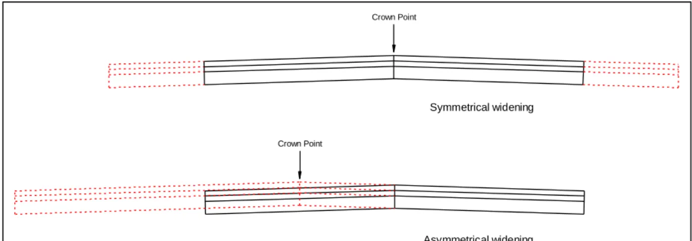
VGU advises that roads narrower than 13 m wide should be widened to 14 m to accommodate the extra traffic lane. Widening techniques, Figure 17, can be classed as either symmetrical or
asymmetrical. The examples show equal pavement widths either side of the crown-point (mid-point) and this is normal for conventional road type design.
Figure 17. Symmetrical and asymmetrical widening – Conventional road type.
A barrier separated road design, however, requires unequal pavement widths either side of the crown-point. In addition, the position of the crown-point will vary when the road changes between single and double lane sections. This is shown in the section examples detailed in Figure 18.
Figure 18. Widening – 2+1 road type.
Crown Point
Crown Point
Symmetrical widening
Asymmetrical widening
Widening for Single Lane Section
Widening for Double Lane Section
10.2. Transition Points
Problems with construction quality can be experienced at the transition points between single and double lane sections. Transitions will often narrow down to near zero at the tie-in point. Examples of these weak problem areas are detailed in Figures 19 and 20.
Figure 19. Weak transition points – Plan view. Hatched marking indicates new widened section
Weak area Tie-in point
Transition (Not to Scale)
Example 3
Widening for Single Lane Section Example 2
Figure 20. Weak transition point (Photo. Terence McGarvey).
Narrow lengths of road pavement will often be structurally weaker than full width sections as it is very difficult to achieve laying consistency and satisfactory levels of compaction. These areas are likely to degrade quicker than the full width sections.
A possible solution, Figure 21, would be to extend the widened section up to or beyond the actual tie in point. However, further consideration must be given to the longitudinal vertical construction joint which will be exposed to traffic.
An option would be to introduce a transverse vertical joint, J1, and hatched road markings. Transverse joints are easier to construct and the road markings would prevent traffic driving over the longitudinal joint, J2.
The following figure describes how to achieve this when existing surface courses are being retained. The method can be easily modified if an overlay of the existing surface course is planned.
Figure 22. Revised construction method.
Longitudinal joint, J3, will still be subjected to traffic loading but will be protected to a certain extent by the surface, binder and base courses.
Construction methods associated with the vertical interface between new and existing pavement construction (longitudinal joint - J4) are discussed in the next chapter.
10.3. Interface between new and existing construction
Vertical interfaces between new and existing construction are considered to be weak points in the road structure. The vertical joint along the existing road crown-point can also be considered as a potential weak point. Ideally, vertical joints should be constructed out-with vehicle wheel tracks; however, this may prove to be difficult for certain recommended section designs.
Figure 23. Widening from 9 m to 13 m (without cycle and pedestrian use).
Figure 24. 2+1 project – Vertical joint positions (A+B) during and after construction (Photo. Terence McGarvey).
It can be seen in Figures 23 and 24 that vertical joint positions can be constructed in or close to vehicle wheel paths and are therefore likely to be subjected to direct trafficking.
To try and improve cross section design, consideration must be given to where in the road vehicles drive. This can be achieved by plotting vehicle average positions and standard deviations.
3 0 0 R o a d E d g e La n e E d g e M a rk in g C e n tr e M a rk in g La n e E d g e M a rk in g G a u rd ra il La n e E d g e M a rk in g La n e E d g e M a rk in g R o a d E d g e K1(d) K2(d) K1(s) 3500 3250 3750 4000 New construction Vertical joints within wheel track 9000 Existing construction Existing crown point 500 450 750 500
Typical Section for Widening of Existing 9m Road - Double Lane Section (without pedestrian and cycle use)
11.
Vehicle Position
11.1. Plotting vehicle position
To confirm where vehicles are driven in a lane, data from the vehicle lateral position surveys was used to map vehicle front tyre average positions and associated standard deviations. As tyre contact widths were unknown, widths of 175 mm (205 tyre size) for light vehicles, and 265 mm (295 tyre size) for heavy vehicles have been assumed and used in the calculations.
Normal distributions are symmetric and have bell-shaped density curves with a single peak. This is like the distribution pattern observed with vehicle position (Appendix 8). Two quantities must be specified: the mean (𝑥̅), where the peak of the density occurs, and the standard deviation (s), which indicates the width of the curve.
The example below (Figure 25), shows how average positions (𝑥̅) and standard deviations (s) can be used to estimate the probability of where in the road a particular group of vehicles are driven.
Figure 25. Distribution of light vehicle position. (McGarvey, 2016)
By applying the three-sigma rule, it can be assumed that nearly all tyre positions will be contained within three standard deviations of the average tyre position. The example above shows that off-side tyre positions are confined within a 1 711 mm band width. Near-side tyre positions are confined within a 1 765 mm band width.
11.2. Surveyed average positions and standard deviations
The following scaled drawing examples show the average tyre positions (full line) and associated standard deviations (dash line). Green lines indicates light vehicles and blue lines indicates heavier commercial traffic.
Example 1: Road 34 – Survey locations A1 and A2
Figure 26. Road 34 - Survey locations A1 and A2.
In this case, the presence of side guard rail, on both sides, has pushed the traffic position to the left. Almost all traffic in the single lane section (within three standard deviations) was confined within the traffic lane.
A large percentage of traffic in the double lane section was positioned close to the mid-point between the two lanes.
Lateral wander was much more confined in the single lane section.
HGV track assuming a front tyre contact of 265mm
Light vehicle track assuming a front tyre contact width of 175mm Road 34: Surve y Location A2 and A1
S id e G a u rd ra il L a n e E d g e M a rk in g L a n e E d g e M a rk in g C e n tr e G a u rd ra il L a n e E d g e M a rk in g S id e G a u rd ra il L a n e E d g e M a rk in g (Motala) (Motala) (Linköping)
Example 2: Road 34 – Survey locations B2 and B1
Figure 28. Road 34 - Survey locations B2 and B1.
The above example shows that the narrow verge width has pushed traffic in the single lane section to the left. Almost all traffic was confined within the lane width.
Traffic position in the double lane section was very central. A smaller percentage of traffic, compared with locations A1 and A2, was positioned over the mid point of the two lanes and over the side lane edge marking and verge.
Lateral wander was much more confined in the single lane section.
Figure 29. Road 34 - Survey locations B2 and B1 (Photo. Terence McGarvey).
(Motala) (Linköping) (Linköping) L a n e E d g e M a rk in g R o a d E d g e C e n tr e G a u rd ra il L a n e E d g e M a rk in g L a n e E d g e M a rk in g R o a d E d g e L a n e E d g e M a rk in g
HGV track assuming a front tyre contact of 265mm
Light vehicle track assuming a front tyre contact width of 175mm Road 34: Survey Location B2 and B1
Example 3: Road 636 – Survey locations C1 and C2
Figure 30. Road 636 - Survey locations C1 and C2.
Here, traffic was positioned slightly to the right in the double lane section. A small percentage of traffic was positioned over the mid point of the two lanes.
Traffic position in the single lane section was also right of centre. A small percentage of vehicles were positioned over the side lane edge marking.
Lateral wander was much more confined in the single lane section.
Figure 31. Road 636 - Survey locations C1 and C2 (Photo. Terence McGarvey). (Linköping) L a n e E d g e M a rk in g (Vikingstad) (Vikingstad) R o a d E d g e L a n e E d g e M a rk in g L a n e E d g e M a rk in g C e n tr e G a u rd ra il R o a d E d g e L a n e E d g e M a rk in g
Road 636: Survey Location C1 and C2
Light vehicle track assuming a front tyre contact width of 175mm
Example 4: Road 636 – Survey locations D2 and D1
Figure 32. Road 636 - Survey locations D2 and D1.
Traffic in the double lane section was positioned slightly to the left. A larger percentage of traffic, compared with location C2, was positioned over the mid point of the two lanes.
Traffic position in the single lane section was positioned right of centre. A larger percentage of traffic, compared with location D1, was positioned over the side marking and verge.
Lateral wander was much more confined in the single lane section.
Figure 33. Road 636 - Survey locations D2 and D1 (Photo. Terence McGarvey).
By comparing these vehicle position examples with typical cross section examples, it can be concluded that a significant number of vehicles will be driven over the longitudinal vertical joint interfaces formed between new and existing construction. To minimise the effect of this trafficking, improvements to the cross-section design must be made.
(Linköping) (Linköping)
Light vehicle track assuming a front tyre contact width of 175mm
HGV track assuming a front tyre contact of 265mm
Road 636: Survey Location D2 and D1
(Vik ingst ad)
L a n e E d g e M a rk in g R o a d E d g e L a n e E d g e M a rg in g C e n tr e G a u rd ra il R o a d E d g e L a n e E d g e M a rk in g L a n e E d g e M a rk in g
11.3. Wide side-verge example
An ideal barrier separated road design should provide sufficient lane and verge widths to minimise traffic confinement in the single lane sections. The design should also ensure that vertical joints, between the new construction and existing structure, are positioned out with vehicle wheel tracks. The positive effect associated with a wide side-verge can be demonstrated in the following example. The road has been constructed with a wide side-verge along most of the single lane sections.
Figure 34. Road 22, Single lane section with wide side-verge (Photo. PMSv3, Trafikverket).
Comparisons of rut depth values showed that development rates are very similar in both single and double lane sections. This could indicate that the amount of vehicular lateral wander is similar in the single and double lane sections, and that no accelerated degradation is taking place.
11.4. Cross section design improvements
Using the vehicle position information described in chapter 11.1 as a template, it was possible to modify the typical cross sections recommended in VGU:
Option 1: Widening for double lane section
Figure 36. Option 1 – Widening for double lane section.
Typical distribution of wheel tracks (based on Road 34, survey locations B2 and B1): • Light Vehicle Track (green) assuming a front tyre contact width of 175 mm • Heavy Vehicle Track (blue) assuming a front tyre contact width of 265 mm
In this example, figure 36, the vertical joint at binder course level is placed between lanes 1 and 2 of the double lane section. Surface course and base course vertical joints will be formed 300 mm either side of this point. The existing width of 9.00 m is not sufficient to meet VGU recommendations, so a reduction in Lane 1(s) verge width* (1.00 m to 0.80 m) is required. Alternatively, additional widening on this side will be necessary.
Proposed section widths = (1.00) (3.50) (3.25) (0.45) (0.30) (0.75) (3.75) (0.80*) = 13.80 m Wheel tracking in Lane 1(d) is positioned almost central, however, a significant number of heavy vehicles will still be driven directly over the vertical joint zone - the base course vertical joint is positioned between one and two standard deviations of the HGVs average position.
This design can be further improved in Option 2.
450 300
3500 3250 3750
4800 9000
New construction Existing construction (9m)
1000 750 800* R o a d E d g e R o a d E d g e La n e E d g e M ar k in g La ne E d ge M a rk in g C e nt re M a rk in g La ne E d ge M a rk in g La ne E d ge M a rk in g G a u rd ra il Lane 1(s) Lane 2(d) Lane 1(d)
Vertical Joint Zone - Avoid Trafficking
Existing crown point
Option 2: Widening for double lane section
Figure 37. Option 2 – Widening for double lane section.
Typical distribution of wheel tracks (based on Road 34, survey locations B2 and B1): • Light Vehicle Track (green) assuming a front tyre contact width of 175 mm • Heavy Vehicle Track (blue) assuming a front tyre contact width of 265 mm
This example, figure 37, is similar to Option 1 apart from Lane 1(d) width which is increased by 0.20 m to 3.70 m.
Similarly, an existing width of 9.00 m is not sufficient to meet VGU recommendations, so a reduction in Lane 1(s) verge width* (1.00 m to 0.80 m) is required. Alternatively, additional widening on this side will be necessary.
Proposed section widths = (1.00) (3.70) (3.25) (0.45) (0.30) (0.75) (3.75) (0.80*) = 14.00 m
Assuming that the wheel track distribution in Lane 1(d) will remain the same and the central position is maintained, the vertical joint position at base course level will now be nearer to the second standard deviation point. This means that a lower percentage of HGVs will be driven over the vertical joint zone.
Comparisons with survey location B2 show an improvement of around one standard deviation.
450 300
3700 3250
1000 750 3750 800*
5000 9000
New construction Existing construction
R oa d E dg e La ne E d ge M a rk in g La ne E d ge M a rk in g G a u rd ra il La ne E d ge M a rk in g R oa d E dg e La ne E d ge M a rk in g C e nt re M a rk in g .239 Lane 1(s) Lane 2(d) Lane 1(d)
Vertical Joint Zone - Avoid Trafficking
Existing crown point.
Option 3: Widening for single lane section
Figure 38. Option 3 – Widening for single lane section.
Typical distribution of wheel tracks (based on Road 34, survey locations B2 and B1): • Light Vehicle Track (green) assuming a front tyre contact width of 175 mm • Heavy Vehicle Track (Blue) assuming a front tyre contact width of 265 mm In this example, figure 38, the base course vertical joint is placed at the edge of Lane 1(s). Assuming an existing width of 9.00 m, the total width would be 14.35 m.
Proposed section widths = (1.00) (3.75) (0.95) (0.30) (0.45*) (3.25) (3.70) (0.95*) = 14.35 m
*Widths can be adjusted to ensure that existing crown-point is positioned between Lane 1(d) and Lane 2(d) 450 30 0 3750 3250 3700 1000 950 950 5350 9000
New construction Existing construction (9m)
R o a d E d g e La n e E d g e M ar k in g C e nt re M a rk in g La ne E d ge M a rk in g G au rd ra il La ne E d ge M a rk in g R oa d E dg e Lane 2(d) Lane 1(d) Lane 1(s)
Vertical Joint Zone - Avoid Trafficking
Existing crown point Critical Point
Option 4a: Combined single and double lane design
A combination of design options 2 and 3 could provide an ideal solution with regards to placement of joints. This would result in varying road width between 14.00 m and 14.35 m, however, the 1.00 m wide verge in design option 2 could be widened to 1.35 m to give a constant 14.35 m construction width. The single lane section (bottom right in Figure 39) is however restricted to 5.30 m.
Figure 39. Option 4a – Combined single and double design.
K1(s)
K1(d) K2(d) K1(s)
9000 Existing Cons truction 5350 New C onstruction
5350 New C onstruction 9000 Existing Construction
Transition Length (Not to scale) K2(d) K1(d) G a u r d r a il ( 3 0 0 ) G a u r d r a il ( 3 0 0 )
*Widths can be adjusted to ensure existing c rown point is positi oned bet ween K1 (d) and K2 (d)
5700 3750 3250 3700 1000 950 5300 1350 3700 3250 450 750 3750 800 950* 450* Exis ting crown point Verti cal Joint Zone
Option 4b: Combined single and double lane design
To widen the single lane section (bottom right in Figure 40), the vertical joint zone between new and existing construction can be moved further into lane 2 of the double lane section. As most vehicles in lane 2 are likely to be light vehicles, this may be an acceptable compromise.
Figure 40. Option 4b – Combined single and double design.
The extent of degradation associated with trafficking of longitudinal vertical construction joints is unknown. Workmanship standards, bonding interaction between surfaces, and compaction levels will vary along the length of the joint. Accelerated degradation testing using a Heavy Vehicle Simulator (HVS) may provide useful information on this problem.
5350 New C onstruction 9000 Existing Construction
Transition Length (Not to scale) G a u r d r a il ( 3 0 0 ) 5700 3750 3250 3700 1000 950
9000 Existing Cons truction 5350 New C onstruction G a u r d r a il ( 3 0 0 ) 3700 3250 5650 3750 1000 450 900 1000 450* 950*
Verti cal Joint Zone - Avoid Traffi cking
Exis ting crown point Lane 1(s) Lane 2(d) Lane 1(d)
Lane 1(d) Lane 2(d) Lane 1(s) *Widths can be adjusted to ensure existing c rown point is positi oned bet ween K1 (d) and K2 (d)
11.5. Reductions in recommended design widths
Amendments to standard designs are often required to overcome specific engineering difficulties. In other cases, amendments may be motivated by financial reasons. Amendments may include the replacement of 2+1 sections with 1+1 sections. They may also include width reductions in the cross-section design. Deviations from recommended design widths will influence vehicle position and amount of lateral wander. If these effects reduce the amount of lateral wander, degradation rates are likely to accelerate.
For conventional road design, the following diagram (for light vehicles) shows that decreases in lane width reduce the standard deviation value. It is possible that this trend will also apply to the single lane and double lane sections in a barrier separated road.
Figure 41. Average position standard deviations (refer to Chapter 6).
However, with barrier separated road design, lane width is not the only confining factor. The total width, between road edge and central barrier, also influences vehicle position and the amount of lateral wander. Total width, for single lane sections, can vary between 4.75 m and 5.00 m for conversions of existing 13 m wide roads. Total widths for widened or new constructions are recommended to be 5.50 m or 5.70 m.
The values for lane 1(s) in the above figure are associated with total widths between 5.10 m and 5.20 m. If a recommended width of 5.70 m had been constructed, standard deviation values would possibly have increased to around 300 mm. This extra deviation will increase lateral wander and reduce surface wear and deformation. This design width is possible and is detailed in figure 40.
11.6. Conclusion
The main problems associated with barrier separated road type design are: • Increased confinement of traffic in the single lane sections
• Longitudinal vertical joints positioned under the offside wheel tracks
An ideal barrier separated road design should provide sufficient lane and verge widths to minimise traffic confinement in the single lane sections. The design should also ensure that vertical joints, between the new construction and existing structure, are positioned out with vehicle wheel tracks. A single lane section width of 5.70 m will help reduce the effects of traffic confinement and will ensure that vertical joints are placed out with vehicle wheel tracks.
Placement of longitudinal vertical joints, between lanes 1 and 2, in the double lane section will never be ideal. It is impossible to eliminate trafficking over these joints. Consideration should, however, be given to a wider 3.70 m lane in lane one of the double lane section.
The design should also take into consideration the longitudinal alignment, especially at transition points between single and double lane sections. Weak “triangular” shaped tie in sections should be avoided where possible.
It is very difficult to produce a standard cross or long section design that will meet all requirements. For example:
• Asymmetrical design provides the best longitudinal design but will require a longitudinal vertical joint in lane two of the double lane section.
• Widening for the single lane sections will provide the best solution for reduced confinement and longitudinal vertical joint placement but will require “triangular” shaped tie in sections. Vehicles driving in lane 1 will also require to manoeuvre either right or left at each transition point.
• If no overlay of the existing surface is planned, then widening for the double lane section will provide the easiest solution. However, this design will also require “triangular” shaped tie in sections. Vehicles driving in lane 1 will also require to manoeuvre either right or left at each transition point.
In all cases, the interface between new and existing construction should be used as the start point for design. Consideration should also be given to vehicle types, position in the road, and amount of lateral wander in order to reduce the number of vehicles driving over longitudinal construction joints. If longitudinal joints can be placed out-with two standard deviations of a vehicles average position, only 2.5% of the vehicles will be driven over the joint. A 14.35 m cross section width may prove to be ideal.
12.
Update of VTI Surface Wear Model
Using VTIs surface wear prediction model (Wågberg och Jacobson, 2007) it is possible to estimate surface wear in the single and double lane sections of barrier separated roads.
A similar version of the model is used in PMS Objekt, the Swedish Road Administrations pavement management system.
The following standard deviations are currently used in the surface wear model to describe the variation of average lateral position.
Table 7. Standard deviations according to surface wear model.
Type Road width (m) Lateral Position Std Dev (mm)
1 7 250 2 9 300 3 13 450 4 Wide Road 500 5 Motor Way 250 6 Tunnels 225 7 2+1 Road 200 8 Narrow Road 180
For barrier separated roads, it is recommended that Road type 7 is used in calculations for double lane sections – Lane 1(d) and Lane 2(d). Road type 6 is recommended for single lane sections – Lane 1(s). However, actual measured standard deviations of vehicle lateral position do not match these values. With reference to the following table from chapter 6, vehicles in the double lane section, Lane 1(d), have a deviation value of 365. The deviation value for vehicles in the single lane section, Lane 1(s) is 265.
Table 8. Actual standard deviations according to survey data.
Lateral Position Std Dev (mm)
Lane Lane Width (m) Light vehicle Commercial Vehicle
Lane 1 (s) 3.75 265 270
Lane 1 (d) 3.15 365 230
Using the actual standard deviation values will reduce the amount of estimated surface wear by around 25% in the single lane section and by approximately 40% in the double lane section.
13.
Recommendations and further research
13.1. Design – Conversion of 9 meter road to 2+1
It has been shown that rutting develops quicker in the single lane sections of barrier separated roads. The rutting rate in the double lane sections was comparable with conventional design. It was also confirmed that confinement of vehicles was more severe in the single lane sections. Increasing the total width of the single lane section is possible but this will result in a higher initial investment cost. If an existing road is widened to accommodate the new single lane section (Figure 42), a total single lane width of 5.70 m can be achieved if the total road width is extended to 14.35 m.
Figure 42. Widening for single lane section.
However, when the road structure is widened to accommodate the new lane in the double lane section, a maximum width of only 5.30 m is possible for the single lane section (Figure 43).
Figure 43. Widening for double lane section.
If the vertical joints between new and existing construction are placed further into lane 2 of the double lane section (Figure 44), then the total width in the single lane section can be increased from 5.30 m to 5.65 m.
The joints will be subjected to direct trafficking, but, as most vehicles in lane 2 are likely to be light vehicles, this may be an acceptable compromise.
5350 New Construction 9000 Existing Construction
G a u r d r a il ( 3 0 0 )
*Widths can be adjusted to ensure existing crown point is positioned between K1 (d) and K2 (d)
5700 3750 3250 3700 1000 950 450* 950* 9000 Existing Construction 5350 New Construction G a u r d r a il ( 3 0 0 ) 5300 1350 3700 3250 450 750 3750 800 Ref 1 Ref 2
Figure 44. Widening for double lane section.
This additional width should reduce the confinement effect and therefore reduce the rate of rutting.
13.2. Design – New build 2+1
New build projects should include a minimum cross section width of 14.40 m. This allows for a 3.70 m wide lane to be constructed in lane 1 of the double lane section. This extra width will help to confine vehicle wander within lane and edge markings. The 5.70 m total width in the single lane section should also increase vehicle lateral wander to more acceptable levels.
Figure 45. New build design options with single lane on left side (top) and single lane on right (bottom).
13.3. Design - Road 22, Söderköping to Valdemarsvik
The design used for this road section should also be given consideration. A wide side verge is
9000 Existing Construction 5350 New Construction G a u rd ra il ( 3 0 0 ) 3700 3250 5650 3750 1000 450 900 1000 450 3250 3700 1000 1000 G a u rd ra il ( 3 0 0 ) 3750 950 Ga 3250 37 00 u rd ra il ( 3 0 0 ) 1000 450 57 00 3750 950 14 400 5700 1000 14 400 Ref 3