Groundwater balance and level variation induced by PV and WIND pumping system

THESIS 30 HP

School of Sustainable Development of Society

and Technology (HST)

GROUNDWATER BALANCE AND LEVEL

VARIATION INDUCED BY

PV AND WIND PUMPING SYSTEM

Degree project at Mälardalen University

Student:

Elena Brugiati

Examiner:

Prof. Jinyue Yan

Supervisors:

Dr. Hailong Li

"It is a capital mistake

to theorize before one has data.

Insensibly one begins

to twist facts to suit theories,

instead of theories to suit facts."

Scherlock Holmes

“E’ un errore madornale

teorizzare senza dati oggettivi,

involontariamente uno inizia

ad adattare i fatti alle ipotesi

e non le ipotesi ai fatti”

Scherlock Holmes

i

ABSTRACT

A quick glance at the electrification world map will show that rural areas are in great need of affordable and reliable electricity to achieve development. Renewable energies (RES) are one of the most suitable and environmentally friendly solutions to provide electricity within rural areas. Among the alternative energy sources, solar energy is considered cheap, readily available, nonpolluting and, therefore, promising mean of reducing the consumption of nonrenewable energy sources and sustainable development.

Desertification is one of the main problems plaguing the Chinese grassland. The gradually increasing reduction of vegetation cover causes the soil erosion. Agriculture is an important sector for this country, but unfortunately not much of the land area has good conditions for farming. In this context the irrigation can be a solution to the problem and the use of PVWPS (Photovoltaic Water Pumping Systems) or WPS (Wind Pumping Systems) to produce the electricity for the motor-pumps represents both economic and technical good solution.

Hence, solar energy has a crucial role to exploit water resources in remote areas and to avoid the desertification usually caused by overgrazing.

SIDA research (Swedish International Development Cooperation Agency) fits with this scope, through the specific project “Demonstration and Scale-Up of Photovoltaic Solar Water Pumping for the Conservation of Grassland and Farmland in China”. This project is to integrate renewable Photovoltaic (PV) technology, water-saving irrigation techniques and water resource management to design a robust and user-friendly system to bring benefits to farmers. The goal of this project is to build a PV solar system driven water pump that can pump water from a nearby source to a tank. This work of thesis takes part in SIDA project, and it is focused on groundwater modelling to evaluate water table variations due to the use of PV or WIND water pumping system. The model has been validated matching gathered data from the solar pumping station in Inner Mongolia, China, with the obtained results. The purpose is to create a kind of model useful to carry out several practical evaluations including forecast of future drawdown of the water table.

Groundwater balance has been also carried out with a simple model to determine the available groundwater resource, to provide water for irrigation to halt Chinese grassland degradation without reach the depletion of the aquifer.

The model has been applied to real locations in China in which the water supply match the Alfalfa and pasture grass water demand. The annual cost-benefit analysis has been evaluated in order to verify the economic feasibility of the system.

The new findings of this work show that the modelling is capable of simulating the variation of groundwater after PV pumping system and the effects of future withdrawals in the study area. The matching between the obtained results and the real measurements provides confidence that groundwater modelling is accurate and can positively assist in understanding groundwater systems, enabling planning for future groundwater withdrawals. Moreover, the model used to

ii

drive a simple annual water budget in three different location in China, shows that the groundwater is sustainably exploited for all the three pilot sites as Hohhot, Lanzhou and Quamdo. Available water resources in these areas are able to match Alfalfa and pasture grass water demand without cause the groundwater damage as shown by the results obtained regarding the change in storage. Local condition make it feasible to set up the PV system in the study areas and the project is economically feasible and convenient as highlighted by the economic analysis carried out only for the locality of Quamdo.

iii

TABLE OF CONTENTS

Chapter 1

INTRODUCTION

1.1. Background…………..………..…...1

1.1.1 The SIDA project...2

1.2. Objectives of the thesis...4

1.3. Limitations………...5

1.4. Methodology...5

1.5. Overview………...6

Chapter 2 OVERVIEW OF PHOTOVOLTAIC AND WIND WATER PUMPING SYSTEMS 2.1. Photovoltaic water pumping systems (PVWPS)...8

2.2. Wind pumping for rural areas of the developing countries……..………...9

Chapter 3 BASIC CONCEPTS AND THEORETICAL BASIS OF GROUNDWATER MODELLING 3.1. Aquifer, aquitard and aquiclude…...11

3.2. Aquifers type...11

3.3. Physical properties...13

3.4. Theoretical basis of groundwater modelling……….13

3.5. Steady and unsteady flow.………...14

iv

3.7. Steady-state groundwater flow to pumping wells……...17

3.7.1. Pumping in a confined or semi-confined aquifer………...17

3.7.2. Pumping in a unconfined aquifer...20

Chapter 4 ANALYSIS OF A PUMPING TEST 4.1. The principle...23

4.2. Aquifer test design plan………...24

4.3. The well and the pump………..24

4.4. The measurements to be taken………...25

4.5. Duration of the pumping test...27

4.6. Methods to analyze confined aquifer test data……….…...27

4.6.1. Steady-state flow………..…...28 4.6.1.1 Thiem’s method……….………..……..28 4.6.2. Unsteady-state flow………..……….….………..…..30 4.6.2.1. Theis’s method……….………….30 4.6.2.2. Jacob’s method………...………..32 Chapter 5 RESULTS: GROUNDWATER SIMULATION AND MODELLING 5.1. Trnsys simulation program…...33

v

Chapter 6

FIELD TEST RESULTS: EVALUATING PUMPING TEST DATA AND VALIDATION OF THE MODEL

6.1. Pilot sites………...40

6.2. Description of the systems...40

6.3. Aquifers test data and analysis………...43

6.3.1. Identifying an unknown system...44

6.3.2. Parameter calculation...45

6.3.2.1. System 1………..………45

6.3.2.1. System 2………..………49

6.3.3. Validation of the model………..…….……….………....51

6.3.3.1. System 1………...…52

6.3.3.1. System 2………...…54

6.4. Conclusions...58

Chapter 7 GROUNDWATER BALANCE AT THREE REPRESENTATIVE SITES IN CHINA 7.1. Introduction...59

7.2. Groundwater cycle...60

7.3. Site and data description……….…..………61

7.4. Results………...62

7.4.1. Hohhot, Inner Mongolia……….………..……..62

7.4.2. Lanzhou, Quinghai……….……….……67

vi

Chapter 8

ECONOMIC ANALYSIS

8.1. Outcome...74

8.2. Income...79

8.3. Benefit cost ratio.………..………..…...82

Chapter 9 OVERALL CONCLUSIONS………...……...84 REFERENCES...85 LIST OF TABLES...87 LIST OF FIGURE...89 ANNEX……….………...93

1

1. INTRODUCTION

1.1 Background

Population growth and economic development continue to place increasing pressure on land use, particularly in developing areas of the world. Most often, unfortunately, the areas in need of economic development are areas where the environment is fragile. Desertification is becoming one of the world’s most serious environmental problems. Desertification refers to the formation and expansion of degraded soil. Poor land management, such as overgrazing and over cultivation of dry lands, can easily lead to land degradation and desertification. Increasing population and improper irrigation techniques also contribute to desertification.

In China, and particularly in west China, the over use and the inadequate use of land has contributed to a number of serious environmental problems, especially desertification.

Since the 1970s, overgrazing in the pasture areas has been degrading the ecological system. The combined conflicts among water resources, pasture, and herds make the already fragile ecological system more precarious. Conserving the pasture areas becomes urgent to restore the ecological system in this country. Water conservation in the pasture areas is critical with a focus on developing irrigated pastureland and providing water supply. Nowadays photovoltaic energy is one of the most popular renewable sources since it is clean, inexhaustible and requires little maintenance [3]. The main purpose of this project is the implementation of solar photovoltaic water pumping irrigation systems for pasture land and one of the challenges is the access to electricity to drive pump irrigation because most of the pasture areas are remote and have no access to the electric grid. The pumps driven by PV solar system could be a solution in these remote areas since they operate freely on available sunlight, with no fuel or electrical costs.

For research purposes, engineers and researchers have applied the solar energy for water pumping systems in small areas of the West of China, for the Chinese grassland restoration. The results show that there is a high potential for solar energy pumping and the future of application is promising and also that solar pumping can operate longer and more effectively compared with traditional irrigation technique. The system also directly improves quality of life and promotes socio-economic development in that area. As studies suggest, the grass production might increase 10 times compared to natural grassland [28]. Solar energy, through PV technology for water pumping, can supply both irrigation and drinking water. The great opportunity of this project is:

 to provide a safe and reliable water supply (in terms of quality and water quantity and of independence of energy sources),

 to use an energy source renewable for grassland irrigation and environmentally friendly,

 to have a system with low service costs and

2

1.1.1

SIDA project

The Project will focus on the development and demonstration of solar energy, together with sustainable development of water resources in the pasture areas in Northwestern China. The Project aims to develop a renewable energy-driven irrigation system for conservation of the pasture land. The research will be conducted in the specific project, "Demonstration and scale-Up of photovoltaic solar water pumping for the conservation of grassland and farmland in China".

The Project will:

 increase the productivity of pasture areas;

 reduce overgrazing of natural pastureland and improve the ecological condition;

 develop a market-based system for overcoming the barriers in

institutional arrangements, financial modalities, and policy/regulatory frameworks to allow the model to be replicated and scaled up in the future for conserving pastureland.

The project will be coordinated by steering board consisting of representatives from the partners in the project. The duration of the project will be three years. The budget includes grant from SIDA and in-kind co-funding from the partners in China. The application of solar powered irrigation has significant meanings in China, especially in Northwestern China because the distribution of water resources is uneven and the precipitation is scare in that region as shown in Figure 1.

Using photovoltaic pump system for irrigating the grasslands is very necessary.

3

Figure 2 presents the pilot field study of a 2 kWp PV water pumping systems for the irrigation area of a 4 ha in a remote area, Gangcha County. Due to the time limit, the system optimization and key components (such as water pump and solar PV) have not been designed for the best performance. Anyway some important results have been obtained, such as:

- micro irrigation line is proved to be an effective and water-saving irrigation method in pasture area with little impacts on landscape;

- application of PV driven irrigation system is an effective way for ecological system conservation, production improvement of pasture land;

- the PV irrigation system is suitable for both surface water and groundwater;

- in addition to use the technology for the irrigation of pasture land, it can also be applied for the supply of drinking water for sheep. With the 2000 Wpeak as a package, it can supply water for about 2-4 ha pasture land and 2000 sheep. It can be used for one household or multiple households; - after irrigation the biomass of grass land increase significantly, 4500 kg fresh grass can be increased per ha [7].

4

1.2 Objectives of the thesis

The project presented in this report will be a combination of energy, hydrology and hydraulics engineering and sustainable development in developing countries. The main objectives of this master thesis are:

1. Groundwater modelling through PV and WIND water pumping system simulations with the aim of TRNSYS software.

2. Groundwater annual balance.

The main objectives have been divided in intermediate objectives:

 7 days groundwater modelling through PV and WIND pumped water simulations.

 Identify an aquifer system from pumping test data: to identify an aquifer system, one must compare its drawdown behavior with that of the various theoretical models. The model that compares best with the real system is then selected for the calculation of the hydraulic characteristics [2].

 Evaluate hydraulic properties of the aquifers from pumping test data: when working on problems of groundwater flow, the engineer has to find reliable values for the hydraulic characteristics of the geological formations through which the groundwater is moving. Pumping tests have proved to be one of the most effective ways of obtaining such values [2].

 Dynamic modelling of the groundwater: a model has been created as conceptual descriptions or approximations that describe physical systems using mathematical equations; they are not exact descriptions of physical systems or processes. The applicability or utilization of a model depends on how closely the mathematical equations approximate the physical system being modeled. To evaluate the applicability or utilization of a model, it is appropriate to have thorough understanding of the physical system and of the assumptions applied in the derivation of the mathematical equations [4]. The selected model must be capable of simulating conditions encountered at the site or area. In this master thesis variation of the water level in the well due to the PV and WIND pumping systems has been modeled.

 Validation of the model by comparison with the real data from the field: it is a process of finding out if the product being built is right. That is, whatever theoretical model is being developed, it should do what the user expects it to do.

 Estimates of groundwater recharge at three representative sites in China: These studies are essential for effective management of groundwater, especially when supplies are limited such as in many arid and semiarid areas to halt grassland degradation without reach the depletion of the aquifer.

5

 Economic benefits-cost analysis has been carried out: annual incomes from selling irrigated crop production have been compared to the initial cost of the system including main components of the PVWPS, engineering and installation plus the irrigation system and the well costs. Benefit Cost Ratio (BCR) has been calculated as tool to judge the economic viability of the project.

1.3 Limitations

The assessment has been geographically restricted to northwestern and northeastern of China. Simulations were carried out on the basis of experimental pumping test data identifying a narrow range of possible mean values of transmissivity and storativity. The low accuracy and precision of the measuring instruments used and moreover, some test were false by the local unfavorable conditions. Groundwater flow models are necessarily simplified mathematical representations of complex natural systems. Because of this, there are limits to the accuracy with which groundwater systems can be simulated. These limitations must be known when using models and interpreting model results. Most of the work related to the hydrologic balance is based on a simplified approach: a simple water balance that includes only readily measurable or easy to estimate components has been performed and several assumptions have been done for example on the recharge coefficient. Another assumption that has been done is about the Alfalfa price, since is varying a lot in whole China.

1.4 Methodology

The part of the background has been written using mainly as sources articles and publications, literature and internet, books. The most important work, which has been followed as a guide is “Analysis and Evaluation of Pumping Test Data”, written by G.P. Kruseman -N.A. de Ridder [2]. The pumping test data have been taken from existing studies.

A simple Excel sheet has been elaborated to reproduce the characteristic curves of three different types of aquifer.

The aquifer selected is the one that most approaches to time-drawdown relationships constructed on the basis of pumping test data that have been taken from existing studies.

Excel sheet has been elaborated also to evaluate hydraulic properties of the aquifer and for modelling the variation of groundwater level in observations well induce by PV and WIND water pumping system. Some input data have been obtained thanks to several computer programs: simulated values of PV and WIND pumping flow have been obtained thanks to TRANSYS; weather

6

data have been extracted from CLIMWAT whilst CROPWAT has been used for estimating the crop water requirements; crop production has been simulated with the computer program AQUACROP. Another Excel sheet has been developed to analyze groundwater balance i.e. the analysis of water demand, water supply and change in storage and to analyze the kW peak that is possible to install.

1.5 Overview

The first part of this thesis includes a background about the general problem and the SIDA project; objective, limitation and methodology have been also defined (Chapter 1).

In Chapter 2 photovoltaic and wind water pumping systems have been described in all their basic components.

In Chapter 3 have been described basic concepts and theoretical basis of the model, definitions of aquifer, aquitard, and aquiclude, different types of aquifers, steady and unsteady flow; furthermore Darcy’s law and mass balance equation on which principles of groundwater flow are based, have been described.

Chapter 4 deals with analysis of a pumping test, the principle, aquifer test design plan, the well and the pump, the measurements to be taken and duration of the pumping test. Methods to analyze aquifer test data in three different types of aquifers have been also described in this chapter.

Chapter 5 deals with modelling of the aquifer response from PV and WIND pumping system in two different pilot sites.

Chapter 6 concerns analyzing and evaluating pumping test data from two photovoltaic water pumping systems located in Inner Mongolia. In this chapter have been calculated the aquifer hydraulic parameters, as transmissivity and storativity and the validation of the model has been developed comparing the model obtained by using Theis solution with the measurements carried out during the field experience.

In Chapter 7 accurate estimates of groundwater recharge have been calculated using the mass balance equation at three representative sites in China: Hohhot in Inner Mongolia, Lanzhou in Quinghai and Quamdo, Tibet.

7

In Chapter 9 overall conclusion has been written.

Chapter 10 contains the list of references used to write this work.

8

2. OVERVIEW OF PHOTOVOLTAIC AND WIND WATER PUMPING

SYSTEMS

2.1 Photovoltaic water pumping systems (PVWPS)

In locations where electricity is unavailable or where the use of an alternative energy source is desired, other means are necessary to pump water for consumption. One option is a photovoltaic pumping system. The photovoltaic is a mature technology to convert sunlight into electricity. Solar pumps are used principally for three applications: village water supply, livestock watering, and irrigation.

A benefit of using solar energy to power agricultural water pump systems is that increased water requirements for livestock and irrigation tend to coincide with the seasonal increase of incoming solar energy. When properly designed, these PV systems can also result in significant long-term cost savings and a smaller environmental footprint compared to conventional power systems. Advantages of PV pumping systems include low operating cost, unattended operation, low maintenance, easy installation, and long life. These are all important in remote locations where electricity may be unavailable [7].

Photovoltaic pump are made up of a number of components. The characteristics need to be matched to get the best performance.

The principle components in a solar-powered water pump system include:

 Photovoltaic (PV) panels. The smallest element of a PV panel is the solar cell. Each solar cell has two or more specially prepared layers of semiconductor material that produce direct current electricity when exposed to light. This direct current is collected by the wiring in the panel. It is then supplied either to a direct current pump, which in turn pumps water whenever the sun shines, or stored in batteries for later use by the pump.

 Motor: this can be DC or AC (alternative current). If an AC motor is used then an inverter is also needed. The inverter converts the DC power into three-phase AC power and the current varies continuously as a function of the solar radiation.

 The other major component of these systems is the pump. Solar water pumps are specially designed to use solar power efficiently. Solar pumps use direct current from batteries and/or PV panels. In addition, they are designed to work effectively during low-light conditions, at reduced voltage, without stalling or overheating [9].

9

Figure 3. Example of PV water pumping system for irrigation [9].

The PV array output depends on the intensity of the solar radiation striking the PV array: the more intensively the sun is shining the higher is the power to supply irrigation water while on the other hand on rainy days irrigation is neither possible nor needed. The amount of water delivered by the PV array depends mainly on the amount of the solar radiation received, which depends on the location, the seasonal conditions, the size of the PV array, and the performance of the subsystem.

2.2 Wind pumping for rural areas of the developing countries

Water pumping is one of the most basic and diffuse energy needs in rural areas of the world. It has been estimated that half the world's rural population does not have access to clean water supplies. Where they are used, the demand is for one of the following end uses: village water supplies, irrigation, livestock water supplies. The wind systems that exist over the earth’s surface are a result of variations in air pressure. These are in turn due to the variations in solar heating. Warm air rises and cooler air rushes in to take its place. Wind is merely the movement of air from one place to another. Wind speed data can be obtained from wind maps or from the meteorology office. Unfortunately the general availability and reliability of wind speed data is extremely poor in many regions of the world. However, significant areas of the world have mean wind speeds of above 3 m/s which make the use of wind pumps an economically attractive option. It is important to obtain accurate wind speed data for the site in mind before any decision can be made as to its suitability. The power in the wind is proportional to:

• the area of windmill being swept by the wind • the cube of the wind speed

10

More recently, the pumping of water through small wind-electric systems has become increasingly popular, both due to greater flexibility over mechanical systems and the advantage of being able to use spare electricity for other purposes. Water pumping with wind energy is a type of off-grid system with strong relevance to livestock producers. Most new wind-powered pumping systems use a small wind turbine to power an alternate current (AC) electric pump. The wind turbine is connected to an inverter which converts the produced direct current into alternating current electricity. Wind turbines are often installed in conjunction with solar panels, as the solar array offers predictable performance while the wind turbine can more cost effectively pump larger quantities of water. Systems typically do not involve batteries to store energy, as batteries are expensive and require significant maintenance. Tanks and ponds are used to store water and provide a water supply when the wind and/or solar systems are not pumping water. Figure 4 shows a typical wind-powered livestock watering system in conjunction with solar panels.

11

3. BASIC CONCEPTS AND THEORETICAL BASIS OF

GROUNDWATER MODELLING

3.1 Aquifer, aquitard, and aquiclude

An aquifer is an underground layer of water-bearing permeable rock or unconsolidated materials (gravel, sand) from which groundwater can be extracted using a water well [9].

An aquitard is a geological unit that cannot lead the water through to the surface because of low permeability mostly caused by clay. Clays, loams and shales are typical aquitards.

An aquiclude is an impermeable layer of rock that does not allow water to move through it. Some shale, for example, has such low permeability that they effectively form an aquiclude [10].

3.2 Aquifers type

Aquifers are geological formations that can store, transmit and yield water to a well or spring. There are all kinds of aquifers. The most commonly used types are the confined (or artesian) aquifer, the unconfined (or free, phreatic) aquifer and leaky aquifer. There are also complex aquifer systems consisting of a number of different aquifer types.

Confined aquifer: A confined aquifer (Figure 5) is bounded above and below by an aquiclude. Because of the confining beds, ground water in these aquifers is under high pressure. Because of the high pressure, the water level in a well will rise to a level higher than the water level at the top of the aquifer. The water level in the well is referred to as the potentiometric surface or pressure surface.

Unconfined aquifer: An unconfined aquifer (Figure 6) is characterized by the absence of an aquitard above it but is bounded below by an aquiclude so that the water table forms the upper boundary of the aquifer and is free to move with atmospheric influences such as atmospheric pressure.

Leaky aquifer: A leaky aquifer (Figure 7-8), also known as a semi-confined aquifer, is an aquifer whose upper and lower boundaries are aquitards, or one boundary is an aquitard and the other is an aquiclude. Water is free to move through the aquitards, either upward or downward. If a leaky aquifer is in hydrological equilibrium, the water level in a well tapping it may coincide with the

12

water table. When drilling a hole into the semi-confining layer until reaching the aquifer proper and placing a tight fitting tube, called piezometer, in the hole one may observe that the water level in the tube is either above, at, or below the level of the water table in the semi-confining layer. When the piezometric level is above the level of the water table, the aquifer has an overpressure and groundwater will flow upwards from the aquifer into the semi-confining layer. When, reversely, the piezometric level is below the level of the water table, the aquifer has an under-pressure and there will be downward flow of water (deep percolation, natural drainage) into the aquifer [2].

Figure 5.

Confined aquifer [2].

Figure 6. Unconfined aquifer [2].

13

3.3 Physical properties

The main aquifer characteristics that appear in the equations describing the flow to a pumped well are:

Transmissivity (T): is an aquifer property that allows engineers and hydrologists a mechanism for calculating the amount of water an aquifer system is capable of transmitting across the entire thickness of the aquifer. Transmissivity is defined as the flow rate achievable through a 1-foot section of the aquifer system extending the full thickness of the aquifer under a hydraulic gradient equal to 1 [18].

Storativity (S): characterize the capacity of an aquifer to release groundwater; is a measure of the amount of water released from an aquifer per unit area, per unit change in head. In other words, storativity is an indication of the amount of water that can be removed from an aquifer by pumping. Storativity values are indicators of whether an aquifer is functioning under a confining pressure (confined condition) or water table (unconfined condition) [18].

3.4 Theoretical basis of groundwater modelling

Mathematical models of groundwater flow have been used since the late 1800s.

A mathematical model consists of differential equations developed from analyzing groundwater flow, known to govern the physics of flow. The reliability of model predictions depends on how well the model approximates the actual situation in the field. Inevitably, simplifying assumption must be made in order to construct a model, because the field situation is usually too complicated to be simulated exactly. In general, the assumptions necessary to solve a mathematical model analytically are very restrictive. For example, many analytical solutions are developed for homogeneous, isotropic, and/or infinite geological formations where flow is also steady-state (hydraulic head and groundwater velocity do not change with time). To deal with the more realistic situations (e.g., heterogeneous and anisotropic aquifer in which groundwater flow is transient), the mathematical model is commonly solved approximately using numerical techniques.

When computers first become widely available, numerical models have been the preferred type of model for analyzing groundwater flow and transport.

The first step in developing a mathematical model of almost any system is to formulate what are known as general equations. General equations are differential equations that are derived from the physical principles governing the process that is to be modeled. In the case of groundwater flow, the relevant physical principles are Darcy's law and mass balance. By combining the mathematical relation describing each principle, it is possible to come up with a general groundwater flow equation, which is a partial differential equation (PDE).

14

Since in groundwater studies, the fluxes (Darcy flux, average linear velocity) are macroscopic quantities which are related to the head gradient and hydraulic properties of the aquifer (i.e., porosity, permeability, hydraulic conductivity) by the Darcy's law, the PDE developed for the general groundwater flow is thus established for macroscopic flow in porous media. There are several different forms of the general flow equation depending on whether the flow is two-dimensional or three-two-dimensional, isotropic or anisotropic, and transient or steady state.

3.5 Steady and unsteady flow

There are two types of well-hydraulics equations: those that describe steady-state flow towards a pumped well and those that describe the unsteady-state flow.

In a steady-state flow all fluid flow properties -velocity, temperature, pressure, and density- are independent of time. This means that the water level in the pumped well and in surrounding piezometers does not change with time. Steady-state flow occurs, for instance, when the pumped aquifer is recharged by an outside source, which may be rainfall, leakage through aquitards from overlying and/or underlying not pumped aquifers, or from a body of open water that is in direct hydraulic contact with the pumped aquifer [2]. Unsteady or non-steady flow is one where the properties do depend on time.

It is needless to say that any start up process is unsteady. Unsteady-state flow occurs from the moment pumping starts until steady-state flow is reached. Consequently, if an infinite, horizontal, completely confined aquifer of constant thickness is pumped at a constant rate, there will always be unsteady-state flow. In practice, the flow is considered to be unsteady as long as the changes in water level in the well and piezometers are measurable or, in other words, as long as the hydraulic gradient is changing in a measurable way [2].

In unsteady-flow analysis, two governing algebraic equations must be explicitly solved because the flow and the elevation of the water surface are both unknown. One of the governing equations is the conservation of water volume, and the other is the conservation of water momentum. In steady-flow analysis, the equation for conservation of water volume was trivial because the steady-flows were constant and were used to solve for the flows everywhere in the channel (known elevations were unnecessary). In unsteady-flow analysis, however, a governing equation of conservation of water volume must be explicitly solved for flows and elevations [11].

15

3.6 Darcy’s Law and mass balance

The work is based on the principles of groundwater flow that are embodied in an equation now known as Darcy’s law. Darcy's experiment consisted of a sand-filled column with an inlet and an outlet for water. Two manometers measure the hydraulic head at two points within the column. The sand is fully saturated, and a steady flow of water is forced through it at a volumetric rate of Q [L3/T] [6]. Because the movement of water through the soil sample is slow, the speed of filtration is measured in [m/d]. Darcy’s law states that the rate of flow through a porous medium is proportional to the loss of head, and inversely proportional to the length of the flow path [2]:

Equation 3.1

Where Q is the volume rate of flow (m3_{/d), is is the head loss between the two points within the}

column in m, K is constant of proportionality known as the hydraulic conductivity (m/d), A is cross-sectional area normal to flow direction (m2_{), is the length of the sample expressed in m.}

Alternatively, Darcy’s law can be written as differential form:

(

) Equation 3.2

Where V = Q/A (m/g), which is known as the Darcy velocity and K is a constant of proportionality known as the hydraulic conductivity in the porous medium assumed homogeneous and isotropic. The minus sign (–) indicates that V occurs in the direction of the decreasing head.

It has to be specified that V is the specific discharge and not the real velocity through the sample (pore velocity). Darcy velocity is a fictitious velocity since it assumes that flow occurs across the entire cross-section of the soil sample. Flow actually takes place only through interconnected pore channels.

If we are interested in real flow velocities we must consider the actual paths of individual water particles as they find their way through the pores of the medium.

Hence, should be considered not the area of the entire section, but a reduced area, which takes into account only the pore. This concept can be expressed by the definition of porosity n and can write:

Equation 3.3

Where Vv is the voids volume, and Vt the total volume.

Hence, is possible to define la real velocity of the flow v, as the ratio between the Darcy velocity first calculated, and the porosity:

16

Equation 3.4

then deducting that the real velocity is greater than that of Darcy of a quantity equal to the porosity. The microscopic velocities are real, but are probably impossible to measure.

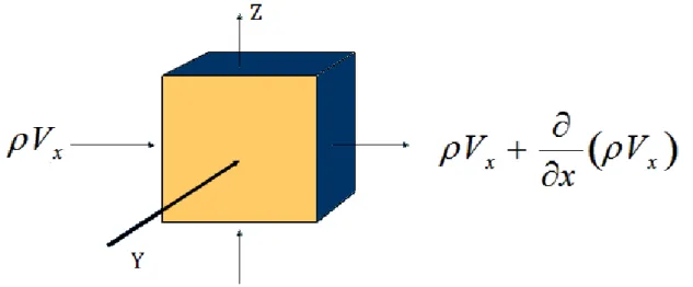
The groundwater flow equation is often derived for a small representative elemental volume (Figure 9), where the properties of the medium are assumed to be effectively constant. A mass balance is done on the water flowing in and out of this small volume, the flux terms in the relationship being expressed in terms of head by using the constitutive equation of Darcy's law, which requires that the flow is slow.

Figure 9. Mass in and Mass out for the mass balance.

(

)

(

)

(

) Equation 3.5

Continuity Equation describes conservation of fluid mass during flow through a porous medium; results in a partial differential equation of flow (Equation 3.5).

If the aquifer has recharging boundary conditions a steady-state may be reached (or it may be used as an approximation in many cases); steady flow means that the flow rate, piezometric head, and amount of fluid in storage do not change with time. Dividing out constant , substituting the Equation 3.2 and assume Kx= Ky= Kz = K can be written as follow:

(

) (

) (

) Equation 3.6

17

3.7 Steady-state groundwater flow to pumping wells

When wells have been pumping for an appreciable time, steady state conditions may prevail. It is only under state conditions that continued drawing of groundwater is feasible. If state conditions are not reached, groundwater levels continue to decline, which finally results in the well falling dry or in a complete exhaustion of the groundwater reservoir.

3.7.1 Pumping in a confined or semi-confined aquifer

Consider a well that is pumping continuously with a constant flow rate Q in a confined or semi-confined aquifer with constant thickness b and homogeneous hydraulic conductivity K. The situation is depicted in Figure 10.

Figure 10. Steady state groundwater flow towards a pumping well in a confined or semi-confined aquifer [12].

Originally, when the well was not pumping the groundwater head was at a level h0, which can be assumed more or less constant in the vicinity of the well. When groundwater is pumped from a well a cone of depression (drawdown) occurs in a confined or semi-confined aquifer as a reduction in the pressure head (potentiometric surface) surrounding the pumped bore. The distance the drawdown cone extends depends primarily on the nature of the aquifer, the pumping rate and the pumping period. Knowledge of the drop in water level and pattern of groundwater flow resulting from well pumping is necessary for assessing environmental impacts in many situations. As the water flows into the well, the water levels or pressure in the aquifer around the well decrease. The amount of this decline becomes less with distance from the well, resulting in a cone-shaped depression radiating away from the well.

18

The flow can be considered completely radial towards the well if the well is screened throughout the entire thickness of the aquifer. Under the following assumptions:

1. The aquifer is confined (semi-confined), 2. The aquifer has infinite aerial extent,

3. The aquifer is homogeneous, isotropic and of uniform thickness, 4. The piezometric surface is horizontal prior to pumping,

5. The aquifer is pumped at a constant discharge rate,

6. The well penetrates the full thickness of the aquifer and thus receives water by horizontal flow.

If qr is the radial groundwater flux at a distance r from the well, it follows from the mass balance equation that the total radial flow towards the well should be equal to the pumping rate:

Equation 3.7

where:

r is the distance from the well (m), b is the thickness of the aquifer (m),

qr is the Darcy velocity (m/d) and the minus sign expresses the fact that qr is negative as it is

directed against the positive sense of the radial axis r.

Using Darcy’s law to express the groundwater flux this becomes:

(

)

Equation 3.8

where T= b· K (m2_{/d) is the transmissivity of the aquifer. From this equation it follows:}

_{Equation 3.9}

This equation can be integrated to obtain an expression for the groundwater head h:

Equation 3.10

where c is an integration constant, whose value can be obtained by stating that at a distance r0 from

19

( ) Equation 3.11

This radius r0 is called the radius of influence (m); it determines the zone in which the pumping well creates a cone of depression and influences the groundwater flow and head. Outside this zone for r > r0 there is no influence and h equals h0. The drawdown s is defined as the difference in

groundwater head due to the pumping well:

( ) Equation 3.12

This equation states that the drawdown is proportional to the pumping rate Q and inversely proportional to the transmissivity of the aquifer. Hence, large drawdown will occur in aquifers with a low transmissivity and for wells with a high pumping rate. This equation also states that the drawdown increases towards the well according to the logarithm of the distance. The maximum drawdown occurs at the well screen and is given by:

( ) Equation 3.13

where sa is the drawdown in the aquifer at the well screen and rw is the outer radius of the well

screen. This equation shows the modest influence of the radius rw, as well as showing, under the

conditions considered, that there is a linear relationship between sa and Q.

The relationship between drawdown and the logarithm of the distance is shown in Figure 11.

20

3.7.2 Pumping in an unconfined aquifer

The second process of flow is one that establishes in an unconfined aquifer due to a fully penetrating well that is pumping continuously with a constant rate Q. The aquifer has homogeneous hydraulic conductivity K. The situation is depicted in Figure 12.

Figure 12. Steady state groundwater flow towards a pumping well in an unconfined aquifer [12]. Originally when the well was not pumping the groundwater table was at a level h0, or H0 above the

base of the aquifer, which can be assumed more or less horizontal in the vicinity of the well. In an unconfined aquifer, the saturated flow thickness, h is the same as the hydraulic head at any location. When the well is pumping a cone of depression is formed that enables groundwater flow towards the well. The flow takes place in the direction of fall of the hydraulic head, h. Pumping from a well causes a decrease of the water table such that the position H of the water table measured from the base of the aquifer becomes variable [12]. The water level in the well defines the top or surface of the zone of saturation; this surface has a pressure that is everywhere the same as atmospheric. The water level inside the well coincides with the piezometric level on the outer surface of the well.

Under the following assumption: 1. The aquifer is unconfined,

2. The aquifer has infinite aerial extent,

3. The aquifer is homogeneous, isotropic and of uniform thickness, 4. The water table is horizontal prior to pumping,

5. The aquifer is pumped at a constant discharge rate,

6. The well penetrates the full thickness of the aquifer and thus receives water from the entire saturated thickness of the aquifer,

21

Equation 3.14

where:

Q is the pumping rate (m3_/d),

r is the radial distance from the well in m, H is the water table position in m,

qr is the radial groundwater flux (m/d).

Using Darcy’s law to express the groundwater flux this becomes:

(

)

Equation 3.15

separating the variables follows:

Equation 3.16

This equation can be integrated between the walls of the well and the undisturbed piezometric to obtain an expression for the water table position H:

( ) Equation 3.17

where:

H0 is the water table original natural position before pumping (m).

r0 is the distance from the well the groundwater table is equal to its original natural position H0

(m).

K is the homogeneous hydraulic conductivity (m/d).

The drawdown s is the difference in water table position due to the pumping well:

Equation 3.18

Carrying out calculations follows:

(

22

This shows that the relationship between drawdown and logarithm of the distance is slightly non-linear; this results from the fact that the drawdown also reduces the transmissivity of the aquifer. With the further assumption that the thickness of the aquifer is considerable, s/2H0 can be

neglected compared to 1, hence:

( ) Equation 3.20

In this case the result becomes identical as for a confined aquifer. The second approach is to define a pseudo drawdown s’ given by:

Equation 3.21

so that:

( ) Equation 3.22

The relationship between the pseudo drawdown, the drawdown, and the logarithm of the distance is shown in Figure 13.

23

4. ANALYSIS OF A PUMPING TEST

4.1. The principle

A pumping test is a practical, reliable method of estimating well performance, well yield, the zone of influence of the well and aquifer characteristics (i.e., the aquifer’s ability to store and transmit water, aquifer extent, presence of boundary conditions and possible hydraulic connection to surface water). A pumping test consists of pumping groundwater from a well, usually at a constant rate, and measuring water levels in the pumped well and any nearby wells called observation wells [13].

The principle of a pumping test is that if we pump water from a well and measure the discharge of the well and the drawdown in the well and in piezometers at known distances from the well, we can substitute these measurements into an appropriate well-flow equation and can calculate the hydraulic characteristics of the aquifer [2]. Pumping tests can last from hours to days or even weeks in duration, depending on the type of aquifer and the degree of accuracy desired in establishing its hydraulic characteristics, but traditional pumping tests typically last for 24 to 72 hours. The obtained data are used to plot drawdown and recovery as shown on Figure 14.

Figure 14. Graph showing the different phases of a constant rate pumping test – the pumping phase and the recovery phase [13].

Pumping test water level measurements should be made prior to, during and immediately following the pumping period (see Figure 14). The information collected during the recovery period is used to verify the results of the pumping test.

24

4.2 Aquifer test design plan

A test design plan will assist the aquifer testing to meet its objectives. Lack of planning can result in delays, increased costs, technical difficulties and poor or unusable data. Factors to consider in aquifer test are:

 Hydrogeological conditions: aquifer type and potential hydrological boundaries.

 time of year the pumping test should be done: aquifer tests are best undertaken outside the irrigation season because pumping from neighboring wells is less likely.

 natural variations in the groundwater levels that occur during the test that needs to be accounted for.

 depth of pump setting and type of pump.

 measuring water levels in neighboring wells and/or streams: wherever possible, nearby wells, especially those closest to observation wells, should not be pumped during an aquifer test.

 measuring pumping rate.

 discharge of pumped water: pumped water must be discharged at sufficient distance and manner so that recharge to the aquifer will not occur.

 pumping duration: to determine later time drawdown parameters in leaky aquifers longer durations are often required.

4.3 The well and the pump

After the well site has been chosen, drilling operations can begin. The well will consist of an open-ended pipe, perforated or fitted with a screen in the aquifer to allow water to enter the pipe, and equipped with a pump to lift the water to the surface. A pumping test does not require expensive large-diameter wells. If a suction pump placed on the ground surface is used, as in shallow water table areas, the diameter of the well can be small. A submersible pump requires a well diameter large enough to accommodate the pump. The diameter of the well can be varied without greatly affecting the yield of the well. Doubling the diameter would only increase the yield by about 10 per cent, other things being equal [2]. The well water is drawn by a pump. The pump and power unit should be capable of operating continuously at a constant discharge for a period of at least a few days. Power needs to be continuously available to the pump during the test. If power is interrupted, it may be necessary to terminate the test, allow the well to recover and run a new test. The capacity of the pump and the rate of discharge should be high enough to produce good measurable drawdowns in piezometers placed far 100 or 200 m from the well, depending on the aquifer conditions [2].

25

4.4 The measurements to be taken

There are three important variables for which accurate records must be kept during an aquifer test: 1. Measurements of the water levels in the well and the piezometers

2. Measurements of the pumping rate from the well 3. Measurements of time.

All may be measured manually or electronically, and accurate records should be retained to allow future analysis and interpretation of test data.

1. The water levels in the well and the piezometers must be measured many times during a test, and with as much accuracy as possible. The most frequent measurements should be at the test start, when the change in depth to water is most rapid. As pumping continues, the intervals can be gradually lessened in frequency. For single well tests (i.e. tests without the use of piezometers), the intervals in the first 5 to 10 minutes of the test should be shorter because these early-time drawdown data may reveal wellbore storage effects. Table 1 outlines measurement frequencies in the pumping well.

Table 1. Recommended minimum intervals for water level measurements for pumping tests in the well [2].

Time since start of pumping

Time intervals

0-5 minutes 0.5 minutes

5-60 minutes 5 minutes

60 -120 minutes 20 minutes

120- shutdown of the pump 60 minutes

Similarly, in the piezometers, water-level measurements should be taken at brief intervals during the first hours of the test, and at longer intervals as the test continues. Table 2 outlines measurement frequencies in those piezometers placed in the aquifer and located relatively close to the well; here, the water levels are immediately affected by the pumping.

Table 2. Recommended minimum intervals for water level measurements for pumping tests in observation wells [2].

Time since start of pumping

Time intervals

0-2 minutes approx. 10 seconds

2-5 minutes 30 seconds

5 -15 minutes 1 minute

15-50 minutes 5 minutes

50-100 minutes 10 minutes

100 minutes-5 hours 30 minutes

5 hours- 48 hours 60 minutes

48 hours- 6 days 3 times a day

26

Table 3. Example of pumping-test data sheet.

Time (min)

s (m)

Water table (m)

400 0 4,64 405 0,02 4,62 410 0,05 4,59 415 0,06 4,58 420 0,09 4,55 425 0,11 4,53 430 0,14 4,5 435 0,16 4,48

2. The pumping rate may be measured in a variety of ways, depending on flow and test requirements. Control of the pumping rate during the test is important as it allows for reliable drawdown data to be collected to determine the yield of the well and aquifer properties. Controlling the pumping rate by adjusting the pump speed is generally not satisfactory. It is better to use a gate valve to adjust the pumping rate to keep it constant. A constant discharge rate, however, is not a prerequisite for the analysis of a pumping test. Aquifers are sometimes pumped at variable discharge rates. This may be done deliberately, or it may be due to the characteristics of the pump. Measuring the discharge of pumped water accurately is also important and common methods of measuring discharge include the use of an orifice plate and manometer or flow meters. If the discharge rate is high, the cone of depression will be wider and deeper than if the discharge rate is low.

Figure 15. Flow meter.

3. Time measurements should be kept as precise as possible. Prior to the test, all water monitoring instruments should be checked to be sure they are working properly. Fresh replacement batteries should be available for all manual sounding probes. Before the test begins, synchronize the watches of all observers. During a constant-rate pumping test the

27

pumping rate must be measured correctly and recorded regularly. In general, the lower the pumping rate, the more accurate and careful the flow measurement must be. An unrecorded change of as little as two per cent in the pumping rate can affect the interpretation of the data, i.e., indicates a false stabilization or a boundary condition.

4.5 Duration of the pumping test

The duration of the pumping test depends on the purpose of the well, the type of aquifer, any potential boundary conditions and accuracy desired in establishing its hydraulic characteristics. Minimum durations of traditional pumping tests are 24 to 72 hours unless stabilization occurs: better and more reliable data are obtained if pumping continues until steady or pseudo-steady flow has been attained. To characterize the hydraulic behavior of a groundwater, aquifer tests shall be used in transient state. These tests are aimed at the determination of the type and aquifer hydraulic parameters characterizing the hydrodynamic behavior of the pumping system. Aquifer tests can all be interpreted under steady-state or unsteady-state, but a complete hydrodynamic characterization necessarily requires the interpretation of the transient test, as under steady-state is not possible to determine the value of the storage coefficient.

There are numerous methods to analyze aquifer test data from multiple wells. The methods that are most accessible for analysis of confined aquifers, and currently most used have been described In this section.

4.6 Methods to analyze confined aquifer test data

When a confined aquifer is pumped, the loss of hydraulic head happens rapidly because the release of the water from storage is entirely due to the compressibility of the aquifer material and the water. This means that the drawdown will be measurable at great distances from the pumping well. Because the pumped water must come from reduction of storage within the aquifer, theoretically, only unsteady-state flow can exist. However, in practice, if the change in drawdown has become negligibly small with time, it is considered to be in a steady-state. Therefore there are methods for evaluating both steady-state flow and unsteady-state flow pump tests.

The assumptions underlying the methods are:

1. The aquifer is confined and the water occupies the entire thickness of the permeable formation;

2. The aquifer has a seemingly infinite areal extent;

28

the test;

4. The piezometric surface is horizontal, prior to pumping, over the area that will be influenced by the test;

5. The aquifer is pumped at a constant discharge rate;

6. The well penetrates the entire thickness of the aquifer and thus receives water by horizontal flow.

And, in addition, for unsteady-state methods:

7. The water removed from storage is discharged instantaneously with decline of head;

8. The diameter of the well is small, i.e. the storage in the well can be neglected [2].

4.6.1 Steady-state flow

4.6.1.1 Thiem’s method

This method is based on the hypothesis of steady-state flow. Thiem was one of the first to use two or more piezometers to determine the transmissivity of an aquifer and it can be used only for confined aquifers. He showed that the well discharge can be expressed as:

(

)

Equation 4.1

where:

Q = the well discharge in m3_/d.

T = the transmissivity of the aquifer in m2_/d.

r1 and r2 = the respective distances of the piezometers from the well in m. s1 and s2 = the respective steady-state drawdown in the piezometers in m.

The following assumptions and conditions should be satisfied: - The assumptions previously listed;

29

Figure 16. Pumping-test in a confined aquifer.

With the Thiem equation the transmissivity of a confined aquifer can be determinated as follows:

(

)

Equation 4.2

The measures may also be carried out using the well in pumping but in this case you have difficulties due to the influence of well losses caused by the flow through the well screen and the flow inside the well to the pump intake.

Hence:

Equation 4.3 where:

is the steady-state drawdown in the well in m. is the radius of the well in m.

Preferably, two or more piezometers should be used, located close enough to the well that their drawdowns are appreciable and can readily be measured.

30

4.6.2 Unsteady-state flow

4.6.2.1 Theis’s method

Theis was the first to develop a formula for unsteady-state flow that introduces the time factor and the storativity. He noted that when a well penetrating an extensive confined aquifer is pumped at a constant rate, the influence of the discharge extends outward with time. Therefore not achieved a balance between flow pumped and depression, and is precisely the evolution in time of the cone of depression to provide the parameters that summarize the hydraulic properties of the aquifers. For this reason this state flow is also called transients, in which it is assumed that the variations of state occur are not in space but also in time.

This method yields the following aquifer characteristics:

 Transmissivity [L2_/T].

 Hydraulic conductivity (where aquifer thickness is known) [L/T].

 Storativity (with an observation well).

The solution of Theis, that relates the pumped flow rate Q at a given time t, starting from the beginning of the pumping with depression s measured at a distance r from the well in pumping at time t, is as follows:

Equation 4.4

where:

s= the drawdown in m measured in a piezometer at a distance r in m from the well Q= the constant well discharge in m3_/d,

T= the transmissivity of the aquifer in m2_/d, and consequently

= the dimensionless storativity of the aquifer, t= the time in days since pumping started.

Equation 4.5

The exponential integral is written symbolically as W(u), which in this usage is generally read ‘well function of u’ or ‘Theis well function’.

31

(

)

Equation 4.6

and the log of 1/u gives:

Equation 4.7

Equations 4.6 and 4.7 show that when observed drawdown is plotted versus t/r2 _{on a double log} graph, this should be similar to a graph of W versus 1/u with only a certain vertical and horizontal translation depending upon the values of Q/4πT and S/4T which are constant.

Figure 17. Analysis of a pumping test according to the method of Theis [12].

Observations s are plotted versus t/r2 _{on double logarithmic graph paper; this is the so called data} graph. Next, W versus 1/u is plotted on similar double log paper, forming the so called type curve or Theis curve. The two curves can be made to match by shifting them vertically and horizontally. In order to determine the vertical and horizontal shifts between the curves a common point is selected on both graphs; this is the matching point and can be arbitrarily chosen as it does not need to lie on the curves. The four coordinates of this arbitrary matching point, smp, (t/r2)mp, Wmp, and (1/u)mp, are the related values of s, r2/t, u, and W(u), noted, which can be used to calculate T and S as:

Equation 4.8

( ) ( )

Equation 4.9

32

4.6.2.2 Jacob’s method

The Jacob method (Cooper and Jacob 1946) is based on the Theis formula, Equation 4.4.

For u < 0.05 the lowest terms of the equation 4.7 can be neglected. It follows that the Theis solution, can be approximated as:

(

) Equation 4.10

This is the approximation of Jacob, which can also be used to analyze a pumping test. In this case observations of drawdown s are plotted versus t/r2 _{on a semi-log graph. Because Q, T, and S are} constant, if we use drawdown observations at a short distance r from the well, a plot of drawdown s versus the logarithm of t forms a straight line as shown in Figure 18.

Figure 18. Analysis of a pumping test according to the method of Jacob [12].

It was observed the drawdown becomes linearly related to the log of the distance from the pumping well and related to the log of the time as well. The slope of the fitted line can be determined by reading the value of Δs on the s-axis corresponding to one log-interval on the log(r)-axis, from which the transmissivity can be calculated:

Equation 4.11

If this line is extended until it intercepts the time-axis where s = 0, the interception point has the coordinates s = 0 and t = t0. Substituting these values into Equation 4.10 gives:

Equation 4.12

33

5. RESULTS: GROUNDWATER SIMULATION AND MODELLING

Figure 19. Groundwater modelling and validation flowchart.

5.1 Trnsys simulation program

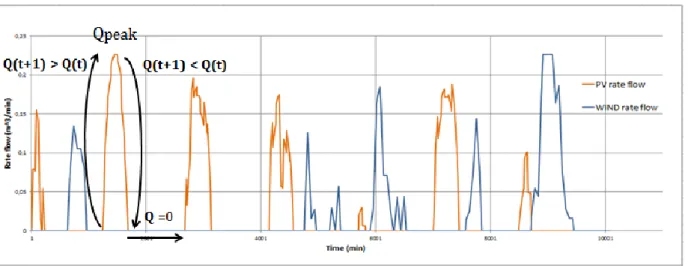
The main goal of the first results part of this thesis is to understand the effects of groundwater withdrawals and potential future withdrawals on water availability which are a major concern of water managers and users. This chapter describes model testing and simulation results for the pumping scenarios posed, so the aquifer response after PV and WIND water pumping system. Simulations of the water flow output from the PV array and WIND turbine were conducted with the use of TRNSYS,

a simulation program with a modular structure primarily used in the fields

of renewable energy engineering and building simulation for passive as well as active solar design. It recognizes a system description language in which the user specifies the components that constitute the system and the manner in which they are connected. The TRNSYS library includes many of the components commonly found in thermal and electrical energy systems, as well as component routines to handle input of weather data or other time-dependent forcing functions and

34

output of simulation results. The modular nature of TRNSYS gives the program great flexibility. TRNSYS is well suited to detailed analyses of any system whose behavior is dependent on the passage of time.

The simulated systems are represented in Figure 20 and consist of solar PV panels and wind turbine, an inverter and a centrifugal multistage pump.

The water is pumped every day with a pump that has a maximum flow rate of 13.6 cube meters per hour. The supply water enters the pump at a constant temperature of 20°C. The pump electrical power is 4 kW. The solar array power is 5 kW.

Figure 20. Simulated system with TRNSYS.

The photovoltaic and the wind turbine are a mature technology to convert sunlight and wind into electricity.

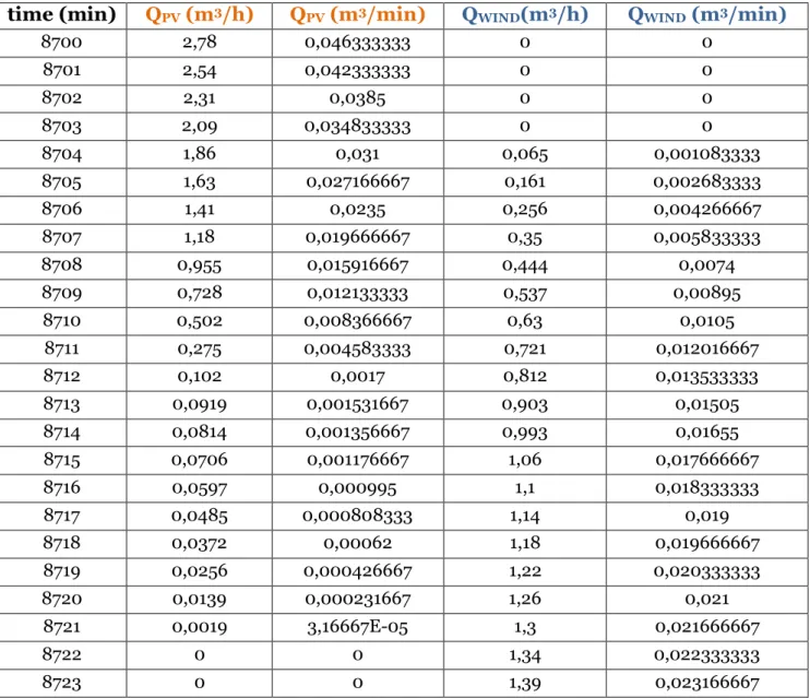
A typical PVWPS consists of a PV array which converts the solar energy into direct current (DC); an electric motor which drives a pump to convert the electrical output into hydraulic power. The water is often pumped from the ground or stream into a storage tank that provides a gravity feed and delivers water to its point of use. The PV array can be directly coupled to a DC motor, or to an alternative current (AC) motor through an inverter [15]. The inverter, 6 kW in this case of study, converts the DC power into three-phase AC power and the current varies continuously as a function of the solar radiation. The system has not distribution networks because sunlight is the only source for electricity generation in such a system. The PV array and WIND turbine output, shown in Table 4 depend on the intensity of the solar radiation striking the panel and the wind caught by the windmill wheel. The amount of water delivered by the PV array depends mainly on the solar radiation received, which depends, in turn, on the location, the seasonal conditions, the size of the PV array, and the performance of the subsystem.