A Deep Learning Approach to Video Processing for Scene Recognition in Smart Office Environments

(1)

Master Thesis Project 15p, Spring 2018

A Deep Learning Approach to

Video Processing for Scene Recognition

in Smart Office Environments

By Karl Casserfelt Supervisor: Radu-Cassian Mihailescu Examiner: Johan Holmgren

(2)

Contact information

Author: Karl Casserfelt E-mail: karl.casserfelt@gmail.com Supervisor: Radu-Cassian Mihailescu E-mail: radu.c.mihailescu@mau.se

Malmo University, Departament of Computer Science

Examiner: Johan Holmgren

E-mail: johan.holmgren@mau.se

(3)

Abstract

The field of computer vision, where the goal is to allow computer systems to interpret and understand image data, has in recent years seen great ad-vances with the emergence of deep learning. Deep learning, a technique that emulates the information processing of the human brain, has been shown to almost solve the problem of object recognition in image data. One of the next big challenges in computer vision is to allow computers to not only recognize objects, but also activities. This study is an exploration of the capabilities of deep learning for the specific problem area of activity recognition in office environments. The study used a re-labeled subset of the AMI Meeting Corpus video data set to comparatively evaluate different neural network models performance in the given problem area, and then evaluated the best performing model on a new novel data set of office activ-ities captured in a research lab in Malm¨o University. The results showed that the best performing model was a 3D convolutional neural network (3DCNN) with temporal information in the third dimension, however a re-current convolutional network (RCNN) using a pre-trained VGG16 model to extract features and put into a recurrent neural network with a uni-directional Long-Short-Term-Memory (LSTM) layer performed almost as well with the right configuration. An analysis of the results suggests that a 3DCNN’s performance is dependent on the camera angle, specifically how well movement is spatially distributed between people in frame.

(4)

List of Figures

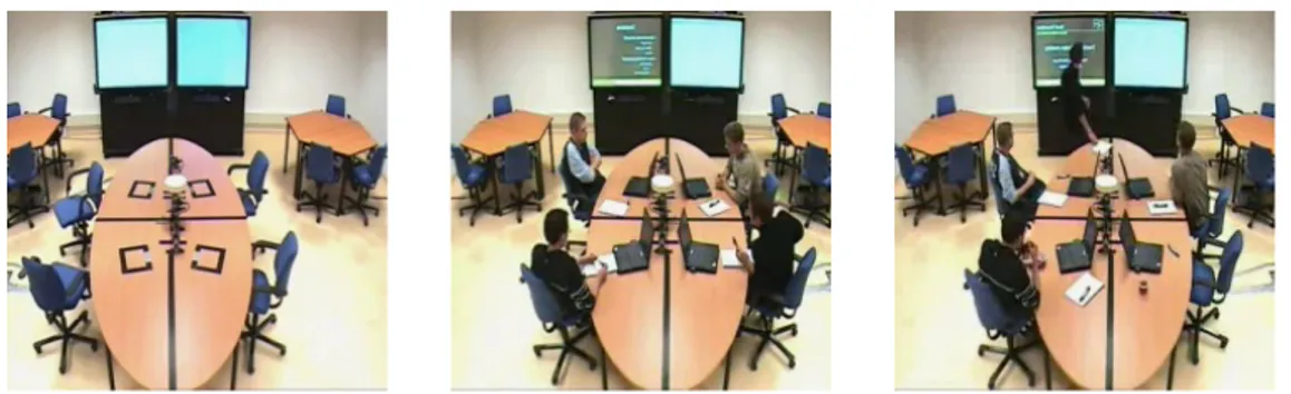
4.1 Images from video clips corresponding with the classes Empty (left), Meeting (center) and Presentation (right). As seen, all images have very similar conditions. . . 40 4.2 Another example of the classes Empty (left), Meeting

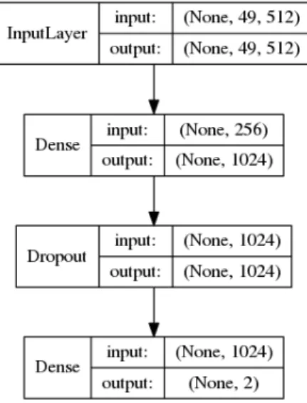
(cen-ter) and Presentation (right) . . . 40 4.3 The final layers that are built on top of the stripped VGG16

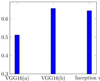
model. Layer type to the left, shape of input and output data to the right. . . 43 4.4 Accuracy scores of CNN training. VGG16(a) uses the VGG16

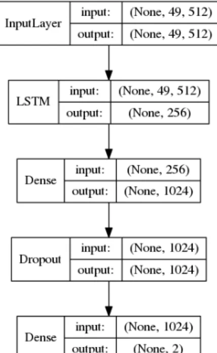
model with random weights, VGG16(b) uses the same model with pre-trained weights from the imagenet dataset, and In-ception V3 uses the InIn-ception model with pre-trained ima-genet weights. . . 44 4.5 The final layers that are built on top of the stripped VGG16

model. Note that an LSTM layer is placed right after input to retain temporal features. Layer type to the left, shape of input and output data to the right. . . 46 4.6 Accuracy scores of transfer learning on VGG16 using normal

CNN technique, and with an RCNN model which included LSTM layer. . . 47 4.7 Figure shows the same scores as in table 4.6, but now with

(5)

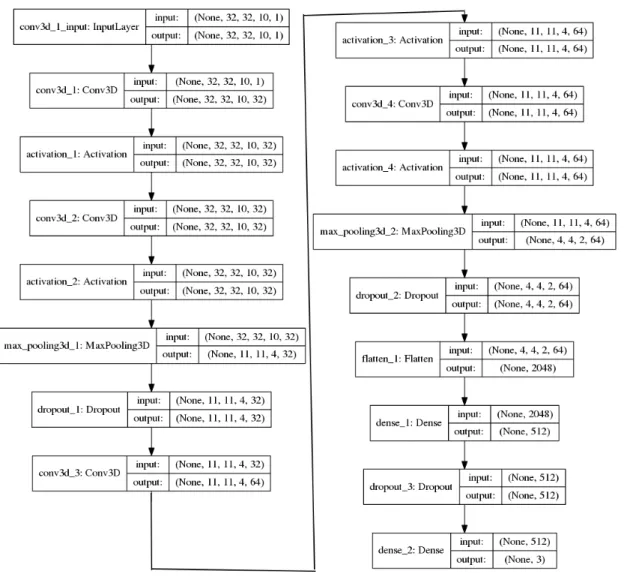
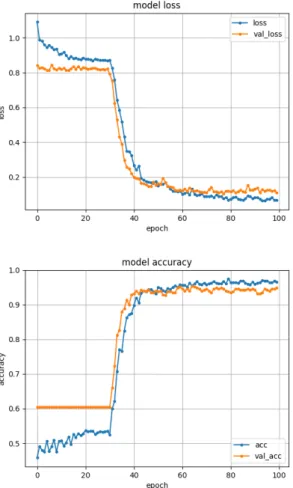
4.8 The 3D CNN model constructed by Fujimoto laboratory in Kobe City College of Technology. [1] [29], used for 3D CNN experiments. . . 51 4.9 The progression of accuracy and loss over 100 epochs of

training on the 3DCNN model . . . 52 4.10 Training progression of different combinations of High/low

dimensions and bidirectional/unidirectional LSTM’s on RCNN with VGG16 . . . 54 4.11 Heat map representation of movements in a meeting and a

presentation in the exact same environment and camera an-gle. Top: A meeting and its heatmap representation. Bot-tom: A presentation and its heat map representation. . . . 59 4.12 Top row: Movement heat map of three meeting scenario

videos. Bottom row: Presentation scenarios from the same room and camera angle as the above image . . . 60 5.1 Examples of frames from the three cameras used in the

con-struction of the IOTAP Activity Data Set. As can be seen, camera 1 (left) and camera 2 (right) have rather similar view-ing angles. . . 64 5.2 An example of two similar situations, but labeled as two

different activities: left depicts a meeting, while right depicts group work. . . 65 5.3 The training progression of a session with all IOTAP data,

and validation data randomly selected. . . 68 5.4 The training progression of a session for the two ceiling

cam-eras, and validation data randomly selected. Camera 1 left, camera 2 right. . . 69 5.5 The training progression of a session with data from the

(6)

5.6 Accuracy progression during training for data from the cor-ner camera (left), ceiling camera 1 (center), and ceiling cam-era 2 (right). . . 72 5.7 The accuracy score of all cameras including combined data,

with random validation and date separated validation. . . . 73 5.8 An example of a meeting captured by the corner camera.

Pay attention to how far away one of the participants are, and that one of the partcipants of the meeting is almost hidden behind the white blinds. . . 75 5.9 An image of a meeting and its movement heat map. . . 76 5.10 An image of group work and its movement heat map. The

activity takes place at the same table as the meeting in figure 5.9, and has a similar distribution of movement. . . 76 5.11 An image of a meeting captured from ceiling camera 2, and

its movement heat map . . . 77 5.12 An image of group work and its movement heat map

cap-tured with ceiling camera 2. Except for the different in move-ment noise coming from lighting changes, the movemove-ment is much more clustered than in the meeting in figure 5.11 . . . 77

(7)

List of Tables

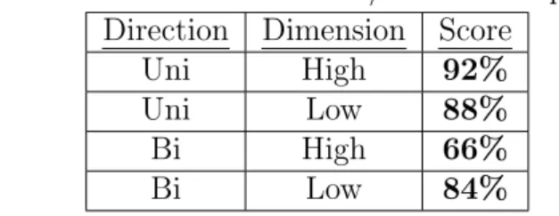
4.1 Overview of results from experiments comparing VGG16 and Inception V3, pre-trained weights and random weights, two class and three class, and RCNN with LSTM using continu-ous and discrete classification . . . 48 4.2 Scores from direction/dimension experiments . . . 55 5.1 The new IOTAP Acitivty data set, and its distribution of

cameras and activities . . . 64 5.2 Summary of all real world experiments with randomly

se-lected validation data . . . 70 5.3 Data distribution of the date separated training/test split.

Note how the quantity of test data is generally smaller than the training data for each class and camera, which was the criteria for picking the dates for the test set. The exception for this is the ’silent work’ and ’meeting’ classes of ceiling camera 1 and one instance in the corner camera. . . 71 5.4 All results from testing on the IOTAP activity data set . . . 73

(8)

List of Acronyms

NN Neural Network

CNN Convolutional Neural Network RNN Recurrent Neural Network

RCNN Recurrent Convolutional Neural Network LSTM Long Short Term Memory

(9)

Chapter 1 Introduction

Ever since the late 1960’s, the dream of giving machines vision in order to view and understand their surroundings have existed both in academia, industry and the general public. Computer vision, as the field later came to be called, was initially seen as a fundamental gap to bridge in order to grant truly intelligent behaviour to robots. [49] Intelligent behavior of machines and computer systems are today more relevant than ever with the emergence and rapid expansion of a myriad of fields with an increasing demand for intelligence, including robotics, automated vehicles, internet of things and smart environments. One of the first attempts to tackle this problem was the Summer Vision Project which took place over the sum-mer of 1966, where researchers and undergrads of MIT set out with the goal of letting computers review images and describe whether the images contained either a ball, a brick or a cylinder. [8] As the project participants would discover, the problem turned out to be a lot more complicated than what was first anticipated. Even though huge advancements in the field of computer vision has been made since the Summer Vision Project, the field is still being heavily researched to this day.

(12)

tune techniques for extracting information from images through means such as pattern recognition, edge detection and texture analysis. However, de-spite such techniques having shown both promise and success, the field has over the past couple of decades increasingly shifted focus into approaching the problem through machine learning techniques. The latest big leap of the field was in 2012 when a research team managed to outperform all other known techniques in object recognition using deep learning with artificial neural networks, which led to a surge in attention and hope given to the technique. [42]

This study aims to explore the field of computer vision in the specific area of office environments, with the aim to let a computer infer and un-derstand what activities are going on in the office using a camera as input device. With its recent promises in mind, the technique employed is of course Deep Learning.

1.1 Deep Learning

Where the conventional way of solving algorithmic tasks can be simpli-fied to the process of writing a function that takes data as an input and produces a known output, the field of machine learning takes an opposite approach. Instead, a function is written that is fed with both input data and its desired output, and produces an algorithm that is expected to solve the problem. By exposing a machine learning model to a large amount of input/output data pairs within a specified problem space, the idea is to continuously improve the algorithm to increase its likelihood of producing the correct output for new input.

Machine learning has been around for many decades, and while some would even say that the foundation of the technique was invented as early as 200 years ago when linear regression first was developed [54], the term

(13)

”machine learning” was first used in 1959 by computer science pioneer Arthur Samuel. [43] The field of machine learning is heavily tied to various mathematical fields such as statistics, probability theory, calculus and lin-ear algebra, and contain a large range of different algorithms and techniques that employ different methods to achieve learning. Such techniques include linear regression, support vector machines, decision trees, and many more. The machine learning technique that today seems to receive the most atten-tion in both academia and industry is the use of artificial neural networks, which is also the focus of this study. Note that the use of neural networks to achieve learning is often referred to as Deep Learning and the terms are often used interchangeably in the context of machine learning.

The first step towards using artificial neural networks was taken in 1943 when the neurophysiologist Warren McCulloch together with mathemati-cian Walter Pitts wrote the first paper on how artificial neurons might work. [17] Through the emergence of computer technology in the 1950s up until today, the concept of artificial neural networks have cycled through various stages of interest and hope in the concept- several times throughout the second half of the 20’th century hope and expectations of the networks has spiked following advancement in the field, and then fallen when the development has not lived up to the exaggerated expectations that built up. [17]

The latest neural network hype occurred in the 90’s when several com-panies invested in the technique, but as before the interest faded when nothing truly revolutionizing came as a result. [50] Since then, and up un-til recently, artificial neural networks were generally thought of as just one of many machine learning techniques. It was in 2012 when this changed during the ImageNet Challenge, a competition where researchers and de-velopers compete in creating machine learning programs to classify images from the gigantic image database ImageNet.

(14)

The previous years, the score of the winning team had incremented rather slowly- the 2010 winners had an error rate of 28% while the 2011 winners got it down to 26%. In 2012 the first neural network was used in the competition, a model which the team called AlexNet after one of its creators, and it won an extremely decisive victory with as little as 16% er-ror rate, which was over 40% better than the next best team that year. [42] What followed was a new period of hype for neural networks, as already the year after most teams were using the technique in the competition and today it is more or less the only technique used.

It is tempting to believe that the neural network fad will die out again, as it has done several times following these types surges in interest. How-ever, previous times when interest have spiked following an advancement in the field, they have been followed by stagnation and later disappointment. This time it is different- the development has continued rapidly and dra-matic increases in performance has kept on coming. Since AlexNet in 2012, the error rate of the winners of ImageNet challenge has kept on reducing fast. Four years later, in 2016 the error rate was down from 0.16 to 0.03, now outperforming human level object recognition. A year later, in 2017, the error rate was again reduced to 0.023, quickly approaching a perfect score and beginning to create a need for a harder challenge. [42]

Many argue that the theoretical upper limit for neural networks as a concept are at least human level performance in any cognitive task as the currently best performing (non-artificial) neural network we know of is the human brain. Despite this it is possible, or perhaps even likely, that artifi-cial neural networks will reach an upper limit of its capabilities in machine learning tasks some day. However, as of now, the technique shows no signs of slowing down. The currently largest bottlenecks for performance is not the technique itself, but the hardware it is ran on and the data it is trained

(15)

with, both of which are items of rapid development. [21] Meanwhile, re-searchers all over the world are spending time improving their network models and applying them to new data and new applications.

1.2 Context Awareness and Smart Office

Environments

The term ”context awareness” encompass a rather broad area of proper-ties with several competing definitions, although most define the concept somewhere close to the intuitive meaning of the phrase. The first to in-troduce context awareness as a concept related to computing was Schilit and Theimer [44] when they in 1994 worked on a map service system that would adapt its behaviour based on location and time. The authors defined context by giving examples of properties that could be taken into account when describing and understanding a context, such as location, identities of people and objects. Others have later suggested even more broad defini-tions of a context, by referring to context as ”environment, surroundings, or situations of either the user or application” [28].

It has been suggested that context awareness in computing can be de-fined as simple as ”acquiring and applying context” [28, 44, 52], or even ”using context” [23]. A more formal and stringent definition on context aware applications is however given by Dey et. al. [7] who defines it as ”a system is context-aware if it uses context to provide relevant information and/or services to the user, where relevancy depends on the users task.” A simple example of such application is mobile phones that automatically dim their screen brightness when detecting a dark environment [44].

(16)

Current trends in the technology industry and computer science re-search include the concepts of Internet of Things and Smart Environments, which are both encompassed and described by the umbrella term Ubiqui-tous Computing. The fields of ubiquiUbiqui-tous computing related to the notion that computing, information and communication technology can be in-corporated ”everywhere, for everyone, all the time” [32]. By introducing information technology to all conceivable objects, and letting such objects exchange their data, some argue that we can create a new paradigm of humans interaction with technology. By having a multitude of objects and systems interact in an environment, new possibilities arise for assisting and aiding the humans in that environment in the best possible way.

Context awareness is an integral part of ubiquitous computing as the added value of interconnected objects and systems largely stems from their ability to adapt to the needs of the users. As Lopes et. al. [32] puts it, ”this new class of computer systems, adaptive to the context, enables the devel-opment of richer applications, more elaborated and complex, exploiting mobility of the user and the dynamic nature of modern computing infras-tructures”. Coming back to the topic of this study, one of the main benefits, and main challenges, of smart environments is to let the system infer the situations of its users by analyzing their context, in order to proactively take measures to assist their needs. [39] Reisse et. al. [39] give an example of a smart meeting room, where the users should not have to connect their laptop to a projector or darken the room themselves if the system infers that they are about to hold a presentation. Rather, the system should do these actions automatically and proactively if it uses the context to under-stand the situation correctly.

It is precisely this problem space that this study is concerned with. While Reisse et. al. [39] propose a solution based on a multitude of objects used to map action sequences through a semantic web, this study will

(17)

approach the problem by using computer vision and deep learning to detect the actions and situations of a smart office environment. If the method proposed in this study proves to be effective in detecting activities in office environment, there are a large number of use cases where the extracted context can be communicated to various subsystems that could proactively assist office workers in their daily activities.

1.3 Motivation and Problem Formulation

The motivation for this study is twofold. Firstly, the project is motivated in part of the general usefulness of context awareness in smart offices, as discussed in the previous section. By contributing to the field of activity recognition, and by extension context awareness, the hope is to further the area of smart environments and bring them closer to practical useful-ness and general adoption. This can ideally aid the development of smart environments as are described in section 1.2. Secondly, while the field of deep learning is rapidly expanding and taking on new problem areas, the limitations of the technique is not entirely known for all problem spaces. With this study, one of the goals is to explore and evaluate how different types and configurations of deep neural networks perform on the problem space of activity recognition in office environments. By giving an account on what factors that prove to be most important in generating the best performance for this problem space, the knowledge produced could ideally provide a foundation for future research in related problem areas.

The benefit of this study is amplified by the fact that very little previous research has had similar ambitions as the ones of this project. The study with the most similar practical outcome was done by Oliver et. al. [35], who wanted to achieve activity recognition in office environments. However they designed an intricate and obtrusive system using a variety of different input methods and had very little focus on computer vision and no focus

(18)

at all on deep learning. Other researchers who has done work in activity recognition using computer vision and deep learning has on the other hand had very different goals than the ones posed in this study. For example, two of the state-of-the-art research papers in activity recognition are done by Ibrahim et. al. [24], who focused on sport videos and general activity, and Karpathy et. al. [26] who only focused on sports videos. The knowl-edge produced by these authors are not very compatible with the project at hand since evidently, the task of distinguishing a table tennis game from a basket ball game has very little in common of the task of distinguishing a meeting from group work using only visual data.

The area of activity recognition in office environments is rather com-plex as a computer vision classification problem. In related areas such as object recognition, the goal is to identify distinct objects in images. Ac-tivity recognition on the other hand is normally performed on data where subjects are moving and interacting. Scene recognition aims to detect and classify the scenes of images. When it comes to activity recognition for of-fice scenarios, relevant information about what is going on can potentially be a rather complex mixture of the three mentioned categories of visual classification. In order to infer whether an activity is for example a presen-tation seminar, it is not enough to identify the activities of individual users but also the combination of activities and interaction between them. At the same time, objects can discern and separate activities from each other. If a user uses a computer it means something else than if they are using a whiteboard. Even scene recognition plays some part in this problem space as a group activity could mean different things if it takes place in a confer-ence room or a break room.

This means that even without the added benefit of improving context awareness in smart offices, this is potentially a study that can produce im-portant knowledge on how to construct neural network models to approach

(19)

this type of complex data. By investigating what types of neural network models and configurations perform best for this problem space, future re-search could gain a better insight as to which point to start from when approaching similar problems.

1.4 Research Question

In order to encompass the entire problem area that is addressed by this project, the research question is rather broadly formulated as;

What performance in terms of accuracy can be reached for activity recognition in office environments using deep learn-ing and video data, and which factors are affectlearn-ing the score?

Of course, this project will not be able to determine the maximum theoretical performance for the problem area given that the score is very reliant on what data is being used for training and validation, together with the fact that it is impossible to test all possible configurations. Rather, what is being researched is what accuracy score that can be reached given the preconditions of the project, such as particular data, time scope and equipment available. With that said, the research question is kept general and broad in order to avoid hindering the development process.

(20)

Chapter 2 Research Method

The research method chosen for this project is Design Science Research, which is also known as Constructive Research. This style of research is by some claimed to be one of the most popular research methods in computer science. [19] The aim of this method is to solve practical problems while producing an academically appreciated theoretical contribution [38], mean-ing in this case that the researcher practically produces a system in order to evaluate the process and reach academic conclusions. The reason for this choice is that the problem that this study aims to approach is indeed practical in nature, with a broad enough scope to not be fitting for a pure experimental design.

However, despite the practical focus of the research, design science does demand both clear scientific contribution and having generalizability in mind. Due to the lack of previous research to depart from, in the case of this project it does seem sensible to also incorporate experiment design as part of both the process and results in order to examine what specific aspects of the implementation that yields the best results. For this reason, controlled experiments will be used in addition to the constructive research.

(21)

2.1 Research Process

Lorenzo et. al. [33] describe the constructive research as that it ”...implies building of an artifact (practical, theoretical or both) that solves a domain specific problem in order to create knowledge about how the problem can be solved (or understood, explained or modeled) in principle”. It is stressed that due to the academic standards of research, the process of constructing an artifact should be viewed as the method itself, while the contribution should be derived from the knowledge that is produced around the problem domain.

Lehtiranta et. al. [30] identify the six steps in conducting design science as follows;

1. A practical problem is selected.

2. The problem area is studied and understood. 3. A solution to the problem is designed.

4. The feasibility of the solution is demonstrated. 5. The contributions of the study is demonstrated. 6. The generalizability of the results are examined.

Kasanen et al. [27] note that ”...although solving a practical problem is at the centre of all constructive research, not all problem-solving ac-tivities should be called constructive research” and provides four elements that should always be included in constructive research. These include; a) practical relevance, b) theory connection, c) practical functioning, and c) theoretical contribution.

(22)

It is also important to note that this method choice lies outside of the traditional division between quantitative and qualitative approaches, and may very well incorporate both. While constructive research is often re-ferred to as a research method, it does comprise process, approach method and data collection. However, as noted this project will also incorporate controlled experiments in order to aid both the design of the artifact as well as the contribution and its generalizability.

This study will be largely comparative, and thus it could possibly take the form of either a comparative study, or pure experimental research. The reason why neither of these methods are chosen, even though they are heav-ily incorporated in the research, is that no other studies have had the same goals as this one so far. This means that there is no previous work to rely on and comparison cases or experiments can not be designed in advance. By using design science research, the task can be treated as a search prob-lem where results will guide the process forward.

With that said, this is not a classical case of design science research ei-ther since the main focus of the study revolves around comparisons between models. This means that while an artifact is indeed constructed during the research process, the main contributions of the study comes from the re-sults of comparative experiments. This means that step 3, 4 and 5 of the design science steps listed above is performed iteratively, and even to an extent interchangeably.

2.2 Practical Considerations

There are several code libraries available for assisting the construction of neural networks and other deep learning models, and it is generally un-common to construct the code from scratch. A few of the most popular libraries for neural network programming are Torch [4], TensorFlow [5] and

(23)

Theano [6]. On top of that, there are also several libraries that builds on top of lower level deep learning backend libraries that aims to make the programming happen on a higher abstraction level. Two examples are TFLearn [16], which uses TensorFlow as a backend, and Keras [2] which uses either TensorFlow or Theano as backend.

For this project, mainly Keras version 2.1.6 is used, combined with some TFLearn due to the widely available and thorough documentation and community support. Both libraries use the GPU enabled version of tensorflow 1.8, which utilizes a GTX 1060 video card for training. The programming language used is Python 3.6.

2.2.1 Design Process

The general structure of the design process follows two discrete steps. First, a set of controlled experiments will be performed on a data set in controlled environment to investigate what model and configuration performs best on the given problem. Then, a new data set will be constructed from real world activity and validate the winning model.

Controlled Experiments

The first stage of the process will use a subset of data from the AMI Meet-ing Corpus dataset [9]. While this data set contains video streams from meeting rooms and office environment, it does not contain all of the activity classes that are indented to be used for the final model. What it does offer instead is very controlled environments where meetings, presentations and no activity (empty) are taking place in the exact same conditions, with the same camera angles, lighting, and even participants.

This data set is used to perform initial experiments to find the best base model for the problem space. As will be evident later, this is a rather

(24)

challenging data set and it is expected that if a model handles it well it should be extendable to more data and classes. The reason for why no data from other sources are mixed in at this stage is to avoid over fitting the model to unrelated conditions and thus creating unreliable or misleading results.

Real World Testing

When a model has been decided from the results of the controlled exper-iments, the model will be tested using a new novel data set captured in the IOTAP lab in Malm¨o University. The data set is captured from four different cameras in the lab recording for seven weekdays, and then manu-ally labeled and sorted into activities. The final model will be trained and validated using this data to review its fitness in uncontrolled scenarios.

2.3 Disposition

The rest of this report will be structured as follows; first the basic the-ory and concepts of deep learning will be explained to give the unfamiliar reader a better understanding of the later sections. Then an overview of previous work in similar fields will be outlined. In the following chapter, the controlled experiments are explained and performed. This section con-tains both results and analysis from the controlled experiments. After that comes a chapter on the real world testing and the data that was collected for the IOTAP activity data set. This chapter also contains both results and analysis of the experiments. Finally, the last chapter provides a summary, threats to validity, conclusion and future work.

(25)

Chapter 3 Theory and Related Work

This chapter will first summarize relevant theory about deep learning and aim to provide an understanding of important concepts of the field. After that, a literature review over previous attempts to address similar problems is presented.

3.1 Theory

3.1.1 Neural Networks

Artificial Neural Networks, in this thesis referred to as only Neural Net-works, are mathematical constructs modeled after the information process-ing mechanisms of the brain. Biological neural networks work by havprocess-ing a very large amount of interconnected nerve cells, called neurons, that pro-cess information by gathering and transmitting electrochemical signals. [20] Artificial neural networks are simplified models of this process, where ar-tificial neurons are built programmatically and process data in a similar fashion as a brain.

(26)

artificial neurons which are also called perceptrons. It can be thought of as a node in a graph, and has a multitude of connections (edges) to nodes before it in the netowrk, providing it with input, and multiple connections (edges) to nodes ahead of it in the networks, to which it outputs data. Each edge has a weight, which transforms the value in some way before it reaches its destination neuron. Each neuron sums up all the weighted values from its input neurons, after which it applies an activation function which transforms the sum. The transformed value are then sent forward in the network to each output neurons of said neuron. [46]

The neurons are placed in layers, ranging from input layer that accepts the input data for the algorithm, and an output layer which represents the final output. If a neural network is used to solve a classification problem, where data belong to distinct categories and the algorithms purpose is to predict what class it belongs to, the output layer often consist of the same number of nodes as there are classes. The node that ends up with the highest value are expected to represent the correct class. There are, of course, variants to this. The term ”deep learning” in the context of neural networks refers to the depth of the network, i.e. how many layers it consists of. [46]

3.1.2 Learning

The way neural networks learn is mainly by passing data with a known output through the network, check what output it should have arrived at, and updating the weight values that transform the input to each node so that the input lands on the correct output. The idea is to do this with a large enough amount of data, that the weight values are fine-tuned enough to reach the correct output for input. If the neural network is successfully trained, it should hopefully be able to generalize the features of the input data that made it correspond to certain output data, and therefore extend

(27)

its capabilities to previously unseen input. This is often done using the Backpropagation algorithm.

The backpropagation algorithm takes each instance of training data and let it flow through the network. For each instance, it computes the error rate of the outputs and works backwards to update the weights to minimize the error rate at each step. Together with backpropagation, a technique called Gradient Decent is used to optimize the model. [46]

Generally, neural networks require a large amount of training data in order to properly learn to produce the correct outputs. It is not uncommon that researchers use hundreds of thousands or even millions of data points in training to create as robust and general performance as possible. To train with this large amount of data usually requires expensive hardware and weeks of time.

3.1.3 Convolutional Neural Networks

Convolutional Neural Networks (CNN) are a specialized type of neural networks which are used in a variety of tasks. However, the area where they have been employed with perhaps the greatest success is computer vision, working with image data. As opposed to classical neural networks as explained above, convolutional neural networks employ what is called convolutional layers in addition to the regular perceptron layers. The way they work is that they use a construct called a kernel which sweeps the data, with the end goal of using pattern recognition to extract high level features in patterns. This is especially useful in image data where patterns such as edges, shapes, colors and more are often vital in recognizing what the image depicts. Instead of passing on shifted values, convolutional layers pass on features of the image to higher layers of the network. In general, the abstraction level of the features increases the further up in the network

(28)

they are. [46]

CNN’s train in a similar way as classical neural networks, where weights and biases are updated through backpropagation, but the direct effect of the updated values are that the convectional layers will adjust their fea-ture extraction to increase the usefulness of their extracted layers. Each convolutional layers is followed by a MaxPool layer which takes input from the convolution and down-samples it. This is done to regularize the image, but also to avoid over-fitting.

CNN’s are currently the best known technique in computer vision and machine learning to infer and classify images and is in some way used in almost all state-of-the-art techniques for image classification. [42]

3.1.4 Recurrent Neural Networks

One limitation with both classical and convolutional neural networks are that they only deal in spatial features. This means that each data point is treated as its own separate instance with no relation to any other input data. In the case of computer vision problems, this means that only one image can be treated at one time, and no data is retained or considered that relates to images before or after it in a series. In the case of video data, the order of frames in a video has significance for the overall interpretation of the video itself. This issue can be addressed by using Recurrent Neural Networks (RNN), which has the capability to deal with temporal data, i.e. data that relates to time. By utilizing temporal data, each data point can be placed in time in relation to any other data point which in turn can provide useful information about the motion in a video.

The way RNN’s work is that they use part of the output from a data point as input to the next one. Since that input itself contains some of the

(29)

output from it preceding data, the algorithm has in theory some informa-tion about all data that so far has been processed in the current sequence. In practice, RNN’s run into issues during backpropagation since gradients are prone to vanish over time, meaning that the memory that is retained can be considered to be rather short-term. [46]

The vanishing gradients can be handled and mitigated by employing what is called a Long-Short Term Memory cell (LSTM), which can be in-serted to a layer of the network. LSTM’s are constructs that uses several gates to treat information, such as input gates, forget gates and output gates. The input gate updates the current state using new input data, forget gates maintains information from previous states, and output gates decide what information should be passed forward to the next state. By using a LSTM, data will either be considered unnecessary and forgotten, or considered important and retained. This leads to a more efficient and longer term memory. [46]

When using video data for classification tasks, it is not uncommon to combine convolutional and recurrent neural networks, creating what is called a RCNN. The idea behind RCNN’s is that convolutional layers will be successfull in extracting useful spatial information about each frame, while recurrent features such as LSTMS are responsible for keeping track of temporal features.

3.1.5 3D Convolutions

As described in section 3.1.3, convolutional networks apply convolutions to pixel matrices to extract features through transformations of patterns in the pixels. An extension of this concept is three dimensional convolutional networks, which work much in the same way except for that they employ 3D convolutions to look for patterns in three dimensions instead of just two.

(30)

Standard convolutions can in principle operate on several dimensions, for example when used on color RGB images with three color channels. How-ever, while these use separate kernels on each layer, 3D convolutions use a different technique to find pattern features related to all dimensions at once.

While the two first dimensions of the input data is the standard width and height of the image, the third dimension represent several different types of data. The two most common are either real depth data, i.e. in addition to the color value of each pixel it contains the distance from the camera, or temporal data which gives information on where the data point exist in the time domain.

By letting the third dimension represent the time domain, both tempo-ral and spatial data can be accounted for in the network, but in a different way than most recurrent networks. Where for example LSTM based re-current models store a history of changes over time, a 3D convolutional network use discrete data points consisting of a sequence of time separated frames stacked on top of each other. Features are extracted in both spatial dimensions as well as the one temporal, but no history can be retained to the next data point.

3.1.6 Transfer Learning and Fine-Tuning

As briefly mentioned in section 3.1.2, training a large neural network can take large amounts of time, and many have trained for several weeks on expensive hardware to achieve state-of-the-art results. For projects that do not have those kind of resources in terms of time, equipment, or train-ing data, common techniques to employ is Transfer Learntrain-ing or fine-tuntrain-ing.

Transfer learning is a technique that means that an existing neural net-work model is used, with all its weights initialized to the values that are a

(31)

result of previous training. Many such pre-trained models exists and are avaliable, and they are often the result of very rigorous training. What then is done is that the last few layers of the model is stripped away and replaced with layers that correspond with the problem space that is being addressed. This almost always include at least a new output layer with the new classes, and the last full connected layer that precedes the output layer. In practice, this means that the original model extracts features from the data, as it is trained to do so, and these features are then used as an input to a new network built on top which is trained using only the high level features as inputs. Even if the original model is not trained to identify the same classes as intended for the new model, it is often still better at find-ing high level features such as shapes or edges than a novel model would be.

Fine-tuning is a technique that is heavily related to transfer learning, and uses the precisely same principle with one exception; where transfer learning only uses the pre-trained weights as is, and uses their output as data, fine-tuning allows for tweaking the weights in the original model. This has the potential of making the collected features more well suited, but also runs a risk of distorting the weights.

Several public deep learning models are available for general usage, many of which has been excessively trained on enormous data sets and shown to perform well. Two of the most popular pre-trained models are the VGG16, and the Inception v3 models, which will be the two pre-trained models used for transfer learning experiments in this study.

Inception V3

The Inception net [48] was created by Google in 2014 and released in 2015. It was created to compete in the famous ImageNet Large-Scale Visual Recognition Challenge, where researchers compete to create the best

(32)

per-forming algorithm to solve large object recognition task. Inception won the ImageNet Challenge in 2015. Inception won the challenge, and has since then been continuously improved. In this study, the third version is used.

The Inception model is built as a very complex network of layers, orga-nized in modules which themselves act as smaller models inside the larger model (hence the name, inspired by the 2010 science fiction film by Christo-pher Nolan). Each module has a multitude of convolutions, each result stacking together. Hence, the technique eliminates the need to decide be-forehand what type of convolutions to perform, making the model more general. [34]

VGG16

VGG16 [47] is sometimes called OxfordNet, is a model created by the VGG group in Oxford in 2014. Where the Inception model won the ImageNet challenge in 2015, VGG16 won the year before. [15]

Much like the Inception model, VGG16 is implementing the concept of modules, although on a somewhat smaller scale than Inception. Some claim that it was VGG16 that popularized sub modules within neural net-work models. [3]

The technical details and precice construction of both Inception and VGG16 are too complex and extensive to disclose in this report, but the main takeaway is that both are very successful convolutions neural networks that both have won the prestigious ImageNet challenge. While both are trained to detect objects and not humans or activities, they are included in this study with the hope of that their excellent feature extraction will aid the activity recognition as well.

(33)

3.2 Literature Review

This section is aimed to provide an overview of both literature and previous research in the various fields that are related to the problem domain of this thesis. As briefly mentioned in the introduction chapter, the area of classi-fying office activities is a rather encompassing domain where both human and group activity, scenes and objects can provide necessary information for successful classification. This means that few previous work efforts are perfectly related to the topic of this thesis, since the exact problem of clas-sifying office activities are not commonly studied.

One attempt to infer office activities were conducted by Oliver et. al. [35] in 2002. Their method for achieving this differs quite a lot from the aim of this project in that they were using three different types of data as input to their model, including keyboard/mouse interaction, captured audio and a camera. The camera however was used to capture and measure the number of people present in the scene which was passed to their model, and the raw pixel data were not used. Neither did they utilize deep learn-ing, but rather Layered Hidden Markov Models, which are a method that is more classically considered to be a statistical model used in probability theory than a typical machine learning algorithm. What makes Olivier et. al. [35] project related to this thesis is that their overall high-level goal were very similar. They were aiming to categorize the office activities in classes such as phone conversation, presentation et cetera. While it is unclear how data were used in their experiments, they reported accuracy scores of up to 99%. This project may not provide any guiding insights for the work on this thesis project, however, it stands to show that the problem area were interesting enough to be addressed already 16 years ago.

When it comes to more practically relevant related work, namely projects that employ deep learning to achieve activity recognition it is clear that

(34)

even in that area, the approaches taken differ quite a bit. Several projects have achieved well functioning activity recognition algorithms using deep learning and non-visual data, such as motion sensor data. Yang et. al [55] achieved very promising results using body mounted motion sensors and deep learning, and displayed a robust model without the need for hand crafted feature extraction. A similar approach was taken by Ronao and Cho [40], who instead of dedicated sensors used smart phones to collect data. Apart from the obvious difference that none of the two mentioned projects used visual data, a key difference from this project is that they did neither classify office activities, nor activities even similar since they focused on single person activity recognition with no regard for scene or interaction. However, they have some aspects to them that are similar to the ambition of this project; Yang et. al [55] achieved robustness and re-moved the need for hand crafted features, which is similar to the goal of using raw video data as an input. Ronao and Cho [40] on the other hand went for a more unobtrusive design, which again is one of the benefits of the proposed solution of this thesis.

However, even though the above mentioned projects give some example to interesting solutions to related problem areas, the most relevant previous work for this project are undoubtedly such projects that address the area of group activity recognition, achieved through visual data and deep learning.

One such article is made by Ibrahim et. al. [24], who achieved state-of-the-art performance in group activity recognition in video data through the use of a hierarchical model that mixes a number of techniques. The authors make use of a tracklet software that first locate and isolate the people in a frame. The areas of the frame that contain people are ran through a convolutional network in order to extract image features, which are then passed through a long short term memory cell (LSTM), one for each person. This is to retain temporal features and relative changes for

(35)

individual subjects. At the same time, features that relate to the group of subjects as a whole are used in another LSTM, and the process is repeated in a two step-process. The authors [24] achieve an accuracy score of 81.5% using this technique when tested on the Collective Activity Dataset [14]. A benchmark was done by fine-tuning the AlexNet pre-trained model and classifying each frame by itself without temporal features, which achieved a 63% accuracy. This shows that the authors significantly improved the scores by introducing their hierarchical model where temporal features were used for both individuals and group separately.

While Ibrahim et. al. [24] have found a both interesting and promis-ing solution to group activity recognition, their problem space differs more from the problem that this thesis project is addressing than what perhaps seems obvious at first. The reason for this mostly stems from the type of data they are concerned with. Both the Collective Activity Dataset [14] and the authors own sports-dataset are picturing activity classes that re-late to a rather high physical mobility. Compare this to most activities in an office setting, such as meetings, presentations or silent work. These type of classes most often imply that very few of the subjects in a video move from their seat. Furthermore, the Ibrahim et. al. [24] solution pre-supposes that the tracklet software for isolating people works as expected and robustly, which may not always be the case for scenarios where users sit down, are immobile or have their back turned to the camera. For in-stance, many methods of finding people in frames are based on background subtraction [53], which relies on people constantly moving in frame. Nev-ertheless, the approach is an interesting one.

Another research team that combines spatial and temporal features in activity recognition tasks are Karpathy et. al. [26], who used a combina-tion of convolucombina-tional and recurrent neural networks to classify activity in the Sports-101 dataset, containing a large number of sports videos. They

(36)

found that the accuracy results that they achieved using spatial features only in classifying the videos frame-by-frame were 59.3%. Surprisingly, the inclusion of temporal features using a RNN only resulted in a very small performance increase, reaching 60.9% accuracy, and their best result achieved 63.9% accuracy. These results are interesting because it is intu-itive that a better result for video classification should be reached with spatio-temporal features. In comparison with Ibrahim et. al. [24], it does seem like the type of data and pre-processing that is used has great signif-icance for the effectiveness of temporal features. Karpathy et. al. [26] also found success in utilizing transfer-learning.

This brief literature review shows that previous state-of-the-art at-tempts to addressing group activity recognition using video data and deep learning have a few factors in common. It seems like convolutional neural networks are used as a foundation in most successful implementation in the field, and they are usually combined with recurrent neural networks to retain temporal features. However, the effectiveness of incorporated temporal features are not guaranteed to yield large performance boosts. Furthermore, both the level of pre-processing and type of data can create variations of accuracy, and it does seem like there are not yet any suggested best practice to approach the problem area of this thesis.

Another take away from this literature review is that all previous work on deep learning and activity recognition has used very different types of activities or input data types in their studies, which means that knowledge previously produces are very hard to adapt to this new problem space. There are a number of previous work in related topics that was not more closely scrutinized in this section. The reason for this is that despite being somewhat similar, they were not deemed to be compatible with this study’s goals and therefore pointless to bring up for other reasons than to point to their differences. All papers reviewed on activity recognition with visual

(37)

data and deep learning were more similar to Karpathy et. al. [26] or Ibrahim et. al. [24] then to this study, such as [18] [13] [31] [51]. Seemingly even more common are articles that uses deep learning for activity recognition, but uses sensor data from warbles, such as [25] [37] [41] [12] [22]. While these are interesting papers in their own, they do not provide any new useful input to the problem area of this study, and strengthens the choice of treating this problem as a comparative search task from scratch, rather than basing it on pre-existing knowledge.

(38)

Chapter 4 Controlled Experiments

As mentioned in the chapter Method, the first step of finding the most suiting model for addressing this problem will be to conduct controlled experiments on the modified AMI Meeting Corpus dataset. The resulting best model from this section is used to test on real world data later.

This section is structured as follows; first the AMI Meeting Corpus data set is presented and the re-structuring and labling of it explained. Then follows a number of experiments using the data, which aims to to test for the best model.

4.1 AMI Meeting Corpus

The AMI Meeting Corpus dataset [9] is a set of recordings from meeting rooms. It includes a large amount of different types of collected data from each meeting session, including video data collected with up to six different cameras, audio data from a multitude of microphones, presentation slides, whiteboard notes and more. For this project, only video data was used. Despite that a number of camera angles were present for each session, only those that had an overview of the entire room were selected to be

(39)

incorpo-rated in the used dataset.

The AMI Corpus dataset has a large bank of annotations for their data, including speech transcripts, social roles and even activities. However, none of the present annotations corresponded well with the aim of this thesis. As such, all video files that were included in these experiments were hand annotated to correspond to one of three classes; ”presentation”, ”meet-ing”, or ”empty”. The reason for selecting these three classes as an initial set of actions to train on comes from the fact that the video files used in the experiments usually had all three of these classes present in the same meeting session. This meant that after annotation and splitting the data, there would be instances of each class where all conditions of the video were exactly the same apart from the activity (or lack of activity). The camera angle, scene, lighting conditions and even people are the same, but their activity differs. This fact would ideally aid in avoiding over fitting the learning model to conditions other than the activity.

The distinction between meetings and presentations were defined as the following: A presentation is counted to occur when all the subjects direct their attention to one person, who is physically separated from the rest. This could be a person standing by a whiteboard, projector or other object, while the rest sit down. A meeting on the other hand is when all subjects have similar poses and physical location (most often sitting at the same table), and have their focus directed to the group.

At this stage, the data is not preprocessed in any way that would assist the classification. While it certainly is possible to do initial image analysis and pass meta features together with the pixel data, this stage is mostly concerned with analyzing how well deep learning models will perform by themselves on the given problem space. The videos are processed in the way that each video frame is extracted into a separate JPEG image and resized to 224x224 pixels, although retaining information on what video

(40)

Figure 4.1: Images from video clips corresponding with the classes Empty (left), Meeting (center) and Presentation (right). As seen, all images have very similar conditions.

they belong to and what position they have in said video. Each video is also copied once and flipped horizontally, creating a mirror image of the original. This was made in order to expand the total volume of data without having to use exact copies of previous data. For experiments where no temporal features were included, and each image was treated as its own discrete data point, random transformations were made during training such as zoom, tilt and crop, again to increase data and decrease over fitting.

Figure 4.2: Another example of the classes Empty (left), Meeting (center) and Presentation (right)

A total of 84 videos were extracted from the AMI Corpus dataset, of which 42 belonged to the Meeting class, 32 to the Presentation class and 10 to the Empty class. All meeting and presentation videos are exactly five minutes long, while the Empty-videos have a varying, but shorter length.

(41)

The reason for that the Empty-class has both fewer and shorter videos were that the original data did not contain as many instances of an empty office, and those which did exist was generally not that long periods. However, this can be considered as a non-issue as a video feed of an empty office is generally not changing and therefore does not require a large variety of data points. However, each recorded session that were used in this project had instances of both meetings and presentations, but not all of them included an empty scene in the same conditions which could potentially become a performance issue.

The videos were split into 25170 images, and 15 percent of each class were dedicated to a test set. Images belonging to the same videos are kept together, again to avoid over fitting.

4.2 System Architecture

The test set up for experimenting with the AMI Corpus Dataset looks like the following; Video files are manually labeled and placed in folders cor-responding to their class. A script is ran that splits all video files into frames, and puts them into a directory hierarchy that represents their class and what video they belong to. At this stage, each frame is resized to a resolution of 224x224 and duplicated as a mirror.

The actual input pipeline differs between experiment. For all experi-ments using VGG16 or Inception, input data is loaded using an instance of Keras Data Generator which automatically shuffles data and delivers data batches. In the 3DCNN experiment, input is handled by 3D numpy arrays of raw pixel data, resized by OpenCV.

Each neural network model is used in the standard Keras implementa-tion unless otherwise stated, and validaimplementa-tion is done by using Scipy to gen-erate a validation set, validated in Keras, and Matplotlib logs the results.

(42)

All models use a learning rate of 0.0001 and image resolution of 224x224, with three channel color with the exception for the 3DCNN, which uses 32x32x10 data with one channel grey scale images.

4.3 Experiments

Here follows a number of experiment done on the modified AMI Meeting Corpus data. Most experiments use the VGG16 or Inception V3 models as a base model since the construction of a novel model is outside the scope of this project, with exception for the testing of a 3DCNN. Factors that are tested for are; transfer learning vs novel training, temporal vs only spatial data processing, structure of data and classes, 3DCNN as an alternative to LSTM, high vs low dimension input features to LSTM, and unidirectional vs bidirectional LSTM’s.

4.3.1 Transfer Learning vs Novel Training

Despite the fact that transfer learning, where pre-trained neural networks are employed and fine tuned in order to solve new problems, are widely considered to be a practical way to leverage previous efforts to reduce computational cost in deep learning tasks, their benefits are not always guaranteed. It does seem likely that this project will benefit from leverag-ing transfer learnleverag-ing, but at the same time there are no widely available pre-trained networks to use that address a similar problem or are trained on similar data. The expectation is that by using a general object detection network as a starting point, it’s pre-trained capabilities of detecting mid-level features such as edges and shapes will aid in classifying the frames of the AMI Meeting Corpus videos.

For this purpose, both the VGG16 [47] and Googles Inception Model v3 [48] will be used as a foundation of transfer learning in this problem.

(43)

While there are many opportunities to tweak the learning process using this technique, for example by specifying what layers that are allowed to update their values in the original models, or building various models on top of the pre-trained layers, this stage will aim to achieve a baseline score of the overall fitness of the technique and the different models. For this reason, all of the layers of the original models are locked from updating their weights and only a simple 3 dense layer model will be built on top of the last non-fully connected layer of the original models.

Figure 4.3: The final layers that are built on top of the stripped VGG16 model. Layer type to the left, shape of input and output data to the right.

Note that these experiments does not take temporal features into ac-count, and thus it treats each video frame as its own image with no relation to the rest of the data.

Three experiments were conducted; one where the VGG16 model were used, and its weights were randomly initialized, one where the VGG16 model were used but the weights used were pre-trained on the imagenet dataset, and finally the inception V3 model with pre-trained imagenet weights. This allows for comparison between transfer learning and original

(44)

training, and between the VGG16 and Inception models. Each experiement were allowed to train for one hour on a GTX 1060 video card.

VGG16(a) VGG16(b) Inception v3 0.3

0.4 0.5 0.6

Figure 4.4: Accuracy scores of CNN training. VGG16(a) uses the VGG16 model with random weights, VGG16(b) uses the same model with pre-trained weights from the imagenet dataset, and Inception V3 uses the Inception model with pre-trained imagenet weights.

As shown in figure 5.7, the pre-trained models outperformed the model that started with random weights by approximately 14-15 percentage units. The VGG16 model with random weights achieved a 51% accuracy, while the same model with pre-trained weights got 65.5%. However, there was a small difference between a pre-trained VGG16 model and a pre-trained Inception v3 model, as the Inception V3 model got 64.4 % accuracy, only 0.9 percentage units below the pre-trained VGG16 model.

A separate test was performed using the VGG16 model with pre-trained weights, but excluding the class Empty so that it became a binary classifi-cation problem between the classes Meeting and Presentation. The reason for this is that the two classes are much more similar to each other than the class Empty, and in the worst case scenario, the accuracy score could

(45)

have been achieved by randomly classifying between the Meeting and Pre-sentation class, achieving a 50 percent accuracy between the two, while classifying the Empty class at an almost perfect score.

The result from this test showed an accuracy score of 67.1%, which disproves the above hypothesis. However, despite that this score is higher than the score for the three class problem, it is important to note that the score is relatively lower than the 65.5% accuracy achieved with the three class problem. The reason for this is that a fully random classifica-tion in a two-class problem still scores 50%, while the number is down at 33% for a three-class problem. Still, the model shows some capability for distinguishing between meetings and presentations already at this stage.

4.3.2 Temporal Features vs Only Spatial

Conventionally in computer vision tasks, temporal features are used when dealing with video data as a sequences of images are the point of using a video. This can also be seen in the literature review where temporal data was always used by similar projects. For this reason, it might seem strange to even do experiments without temporal features on video data in this study. The reason behind it is that the activities depicted are rather inactive in nature, and it does not seem entierly clear that video sequences would provide a better understanding of the activity going on.

Initial experiments with temporal features were set out to investigate the immediate effects the incorporation of RNN elements would have on the performance. For the first experiment in this field, a model was built identical to the best scoring model from the previous section, namely a pre-trained VGG16 model with stripped away top layers, and added one input layer, two dense layers and one dropout layer. The difference in this experiment is that a LSTM layer is added right after the input to the top

(46)

model.

Figure 4.5: The final layers that are built on top of the stripped VGG16 model. Note that an LSTM layer is placed right after input to retain temporal features. Layer type to the left, shape of input and output data to the right.

Somewhat surprisingly, the accuracy score with this model turned out to be considerably lower than what it was with the pure CNN model. The RCNN model with the included LSTM layer only scored a 52.1% accuracy, while the pure CNN model scored 65.5% as outlined in the previous section.

A likely explanation for these results is that while images have their internal order retained within the same video, the order of the videos are randomized. This means that the LSTM is likely to store history from previous videos, which have no relation to the activity in the present video when validating on the test data set. In this experiment, the validation also took place frame-by-frame instead of treating time-separated video

(47)

segments as discrete units. In the literature review, it was clear that the positive effects of using RNN’s in combination with CNN’s were not guar-anteed to be high, but none of the discussed articles reported negative effects. This goes to show that the overall design of the learning model, and the validation, needs to be redesigned with more care as it is very un-likely that the incorporation of an LSTM layer would be inherently unfit for this dataset.

CNN RCNN

0.3 0.4 0.5 0.6

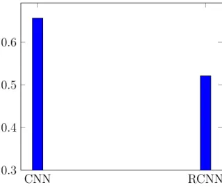
Figure 4.6: Accuracy scores of transfer learning on VGG16 using normal CNN technique, and with an RCNN model which included LSTM layer.

With the above results in mind, the validation step was redesigned to not use the entire dataset as a continuous stream but rather grouping image frames per video and classifying each segment independently in validation. As suspected, this resulted in a much higher accuracy of 88%, outper-forming the corresponding model without temporal features with almost 11 percentage points. This goes to show that temporal features indeed provide value to this problem space, and even produces a substantial im-provement.

An outline of the results this far can be viewed in table 4.1. These initial results provides a foundation for what direction is the best to take

(48)

CNN RCNN RCNN(2) 0.4

0.6 0.8

Figure 4.7: Figure shows the same scores as in table 4.6, but now with the results of RCNN(2) that uses discrete classification.

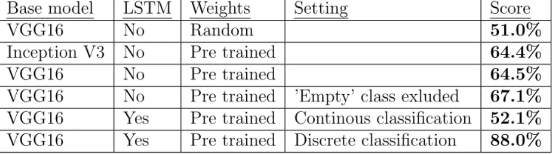
Table 4.1: Overview of results from experiments comparing VGG16 and In-ception V3, pre-trained weights and random weights, two class and three class, and RCNN with LSTM using continuous and discrete classification

Base model LSTM Weights Setting Score

VGG16 No Random 51.0%

Inception V3 No Pre trained 64.4%

VGG16 No Pre trained 64.5%

VGG16 No Pre trained ’Empty’ class exluded 67.1% VGG16 Yes Pre trained Continous classification 52.1% VGG16 Yes Pre trained Discrete classification 88.0%

(49)

to tackle the Corpus Meeting Dataset, as it is shown that VGG16 slightly outperforms Inception V3 as a base model, that pre-trained weights are better than random weight initialization and that temporal feature inclu-sion with LSTM’s makes better results than pure CNN. The experiment where the ’Empty’ class was removed also showed that even a normal CNN was able to at some degree distinguish between the two similar classess ’Presentation’ and ’Meeting’.

4.3.3 3D Convolutional Network

As seen in the results found in previous sections, the tweak that lead to the single largest jump in performance was the inclusion of temporal features by including an LSTM (after making sure that the classification was done discretely on grouped video frames). This strongly suggests that despite the perhaps mild movement done in office scenarios, the movement that does occur provides means for much better distinction between activities and temporal features are vital for successful classification.

As RNN’s with LSTM cells are not the only means of including tempo-ral features in visual data neutempo-ral networks, it does seem viable to explore more options for temporal feature inclusion. For this reason, a 3D Convo-lutional Network was implemented and the data was reprocessed to fit this kind of model.

As mentioned in earlier sections, 3D ConvNets treat sequences of images as three dimensional objects where the images are stacked on each other and the convolutions are performed on the now three dimensional block of pixels. These objects have a width and a height as a normal image, but the depth represent the different frames of the video separated in the time domain. This can lead to very heavy computational tasks that require high end hardware if the input 3D images are not re scaled in all dimensions. In

A Deep Learning Approach to Video Processing for Scene Recognition in Smart Office Environments