Re-processing of reflection seismic data from line V2 of the HIRE Seismic Reflection Survey in the Suurikuusikko mining and exploration area, northern Finland

(1)

Examensarbete vid Institutionen för geovetenskaper

ISSN 1650-6553 Nr 222

Re-Processing of Reflection Seismic

Data from Line V2 of the HIRE Seismic

Reflection Survey in the Suurikuusikko

Mining and Exploration Area,

Northern Finland

Amir Abdi

(2)

(3)

i

Abstract

The Suurikuusikko gold deposit is located in northern Finland; it is the largest known gold resource in northern Europe. The acquired high resolution reflection seismic data along the c.30 km long profile V2 of the HIRE reflection survey in the Surrikuusikko gold mining and exploration area have been re-processed. A 15.4 ton Geosvip was used as the source, with a receiver spacing of 12.5 m and source spacing of 25 or 50 m. It was aimed to obtain more detailed structural information of the upper 5 – 6 km crust, and to study the seismic response of the important geological and tectonic structures (e.g. Suasselkä PG fault) along the line V2. The line V2 runs from south to north; in the north, it cuts the mafic graphitic tuffic rocks, which are buried under a layer of tholeiite. It is almost perpendicular to the surface trace of the Suasselkä PG fault in the north. The obtained seismic image showed significant improvements compared with the previous work. The seismic response of the major rock units generated strong reflections, and they can be traced down to at least 3 km depth; the reflections correlate well with the surface geology. The moderately dipping reflections from the PG fault are clearly imaged; the dip direction of the fault is towards the SE with a dip of about 50o, possibly decreasing with depth down to about 35o, the fault can be traced down to about 3 km depth. The reverse movement of the fault most probably caused the neighboring sub-horizontal layers to be folded and generated a duplex structure. The dip direction of the major structures in the southern parts is towards NE; this together with the mentioned information about the fault, can be utilized in order to define the major geological structures and most importantly the tectonic evolution of the area; such information can be used in many crucial aspects such as prediction of the future movements of the bedrock and discovery of new resources.

(4)

ii

Acknowledgment

It is a pleasure to thank those who made this thesis possible by their contribution and providing me with their valuable assistance in preparation and completion of the paper. This thesis would not have been possible without the help and support of those individuals. I would like to take this chance to show my gratitude towards them.

First and foremost, my sincere gratitude to Prof. Christopher Juhlin, my supervisor for his patience, availability to answer my many questions, his guidance and encouragement throughout the thesis period. It was an honor for me to be advised and guided by him.

I am indebted to Prof. Ilmo Kukkonen, to provide me with significant help in providing data and offering the necessary information which enriched this research. He has always been available for guiding me via e-mail.

GLOBE ClaritasTM under license from the Institute of Geological and Nuclear Sciences Limited, Lower Hutt, New Zealand was used to process the seismic data.

I would like to thank those who guided me with their constructive criticism and useful comments in discussions throughout my research period; namely they are: Dr. Alireza Malehmir, Azita Dehghannejad, Emil Lundberg, Saeid Cheraghi, Peter Hedin and Magnus Andersson. In addition, I was supported by them being available to respond to my questions constantly, which I appreciate so much.

I am grateful to all my classmates who always provided me with their comments and new ideas which helped in improving my work; especially to my dear room-mate, Siddique Akhtar. I am also thankful to my dear friends Mehrdad Bastani and Majid Beiki for their valuable friendship and presence. In addition, special thanks to those who brightened my days with their hope, smiles and positive energy and motivated me in doing a better job. Finally, I would like to take the chance and appreciate my wife, Azin, for all her patience, love and support.

(5)

iii

List of Figures

Figure ‎1.1: General geological map of northern Finland. ... 2

Figure ‎1.2: A simplified loading history. ... 3

Figure ‎1.3: Survey lines in Suurikuusikko... 6

Figure ‎2.1: Main geologic units of northern Finland. ... 8

Figure ‎2.2: Main lithostratigraphic units of central Finnish Lapland. ... 9

Figure ‎2.3: Tectonic map of the Central Lapland Granitoid Complex. ... 10

Figure ‎2.4: Stratigraphy of the Central Lapland greenstone belt. ... 11

Figure ‎2.5: An illustration of the impact of glacial loading and unloading. ... 15

Figure ‎2.6: Distribution of PG faults in northern Fennoscandia... 16

Figure ‎2.7: Location of Suasselkä PG fault in the Kuoko area. ... 17

Figure ‎3.1: Stacking chart. ... 18

Figure ‎3.2: Reflection and refraction of a plane wave. ... 22

Figure ‎3.3: Generated waves at a solid-solid interface. ... 23

Figure ‎3.4: Illustration of down going seismic waves in zero-offset case. ... 25

Figure ‎3.5: A syncline reflecting interface. ... 25

Figure ‎3.6: Geometry of a reflected ray path. ... 26

Figure ‎3.7: Reflector point dispersal. ... 27

Figure ‎3.8: Illustration of the apparent dip in the dipping reflector case. ... 27

Figure ‎3.9: Six fold CMP gather. ... 28

Figure ‎3.10: Zero-offset sections modeled for reflectors with different dipping angles. ... 31

Figure ‎3.11: Travel-time curves recorded for different syncline and anticlines. ... 31

Figure ‎3.12: FD migration. ... 32

Figure ‎3.13: An exaggerated schematic of 2D crooked line profiling. ... 33

Figure ‎4.1: The position of the HIRE line V2 and the CMP lines. ... 35

Figure ‎5.1: A shot gather showing the effect of the refraction static correction. ... 38

Figure ‎5.2: A shot gather showing the effect of the filter. ... 39

Figure ‎5.3: Stacked sections (CMP 3200-4623) before and after DMO correction. ... 41

(8)

vi

Figure ‎6.2: Time-migrated stacked sections for CMP line 1 and 2. ... 44

Figure ‎7.1: The unmigrated stacked sections. ... 46

Figure ‎7.2: Stacked sections A and A’. ... 47

Figure ‎7.3: Stacked sections B and B’. ... 48

Figure ‎7.4: Stacked sections C and C’. ... 49

Figure ‎8.1: 3D illustration of the seismic lines and the surface geology map. ... 52

Figure ‎8.2: Interpreted time migrated section. ... 53

(9)

vii

List of Tables

Table ‎2.1: Summary of stratigraphy of the Central Lapland greenstone belt. ... 12

Table ‎2.2: Summary of CLGB deformation. ... 13

Table ‎2.3: Summary of PG faults within the Lapland Fault Province. ... 16

Table ‎4.1: Acquisition parameters ... 34

(10)

viii

List of abbreviations

CLGB Central Lapland Greenstone Belt

KSZ Kiistala Shear Zone

PG Post Glacial

CMP Common Mid Point

CDP Common Depth Point

NMO Normal Move Out

DMO Dip Move Out

FD Finite Difference

AGC Automatic Gain Control

HIRE High Resolution Reflection Seismics for Ore Exploration GTK Geologian Tutkimuskeskuksen (Geological Survey of Finland)

(11)

1

1. Introduction

1.1. Background

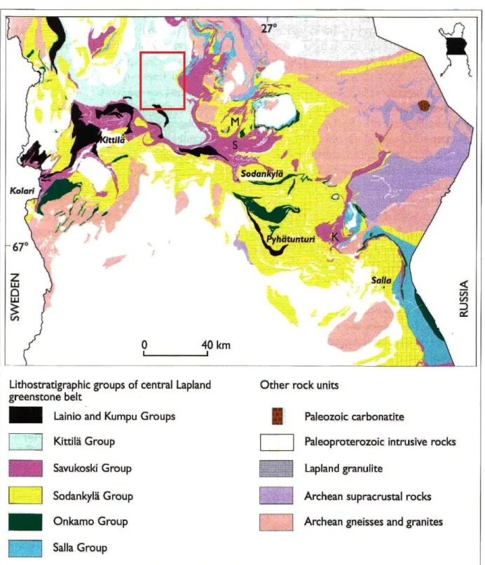
The Suurikuusikko mining area in northern Finland is the largest known gold deposit in the Central Lapland Greenstone Belt (CLGB). It is situated approximately 50 kilometers northeast of the town of Kittilä, and it hosted by the Kittilä Group rocks (Fig. 1.1).

Early discovery research of the Suurikuusikko started in 1980s by the Geological Survey of Finland (GTK) (e.g. Härkönen & Keinänen 1989; Härkönen 1992, 1997; Härkönen et al. 1999a & b).

In 1986 two researchers P. Puhakka and J. Valkama from GTK discovered visible gold SSW of Suurikuusikko. Afterwards the Kiistala Shear Zone (KSZ) was discovered using geophysical and geochemical studies.

Ongoing studies are mostly focused on subjects such as: the exact location of the gold within sulfides, metallurgical presentation of ore, understanding of the host lithologies, structures deformation history and geophysical signature of the deposit (e.g. Bolin & Larsson, 1999; Chernet et al., 1999; Durance et al., 1999; Kojonen & Johanson, 1999; Sandahl, 1999; Kojonen & Pakkanen , 2000; Markström et al., 2000; Markström & Larsson, 2000a & b; Patison, 2000; Sandahl, 2000a & b; Barclay, 2001; Patison, 2001; & Powell, 2001). The diamond drilling by GTK along the KSZ resulted in the discovery of Suurikuusikko. A total of 77 drill holes of about 9,320 meters drilled by 1996, a total resource of 1.5 million tones with an average grade of 5.9 grams per ton have been indicated. The present estimate of the gold production is about 150,000 ounces per annum for 13 years. Better understanding of the geological structures and evolution of the Suurikuusiko area is needed in order to continue successful exploration. (Patison, 2007 and Patison et al., 2007)

The significance of the Suurikuusikko area is not limited to the gold mineralization; the other remarkable characteristic of the area is the existence of the largest Post Glacial (PG) fault in northern Finland (Suasselkä PG fault) which is located close to Suurikuusikko.

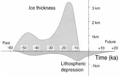
During the past several hundreds of thousands of years loading and unloading of ice in Fennoscandia caused dynamic changes (e.g. vertical and lateral changes in the stress field) in the crust (Fig.1.2) (Pascal et al., 2010). Post Glacial (PG) faulting in Fennoscandia is the result of the last glaciation (Weichselian). The PG faults in Fennoscandia were brought to attention during the 20th century by discoveries in northern Scandinavia (Kujansuu, 1964; Lundqvist and Lagerbäck, 1976; Lagerbäck, 1979; Olesen, 1988).

(12)

2

Figure ‎1.1: General geological map of northern Finland, and gold occurrences in the area. The black rectangle indicates the study area (Fig 1.3). Coordinates according to Finnish National Grid (ykj-grid) metric values (after Lehtonen et al.1998).

(13)

3

The PG faults in Finland gained more value as an interesting subject when the issue of searching for the areas which are suitable candidates for the disposal of nuclear waste was brought up (Kuivamäki et al. 1998). There are at least 14 locations in northern Fennoscandia where the PG faults can be seen (Fig. 2.6).

Figure ‎1.2: A simplified loading history for a site in central Sweden during the last (Weischselian) major glaciation. Ice thickness appears above the time axis and consequent depression of rock below (after Talbot, 1999).

The intra-plate state of stress in Scandinavia mostly represents strike-slip faulting in depth (Juhlin, et al., 2010). The stress regime is mainly considered as the result to either ridge-push from mid-Atlantic (Gregersen, 1992; Slunga, 1991), or both ridge-push and deglaciation (e.g. Bungum, et al., 1996). Moreover, it is most probable that the fault activity is influenced by some other effects such as sedimentary and topography loadings and coastal and mainland unloading pursuant to erosion (Pascal, et al., 2009; Byrkjeland, et al., 2000; Bungum, et al., 2010).

The previous studies on modeling the bedrock stress field during glacial load (e.g., Johnston, 1989; Wu, et al., 1996a; Wu, et al., 1996b; Johnston, 1998; Klemann, et al., 1998; Wu, et al., 1999; Lund, 2005; Turpeinen, et al., 2008; Lund, et al., 2009) showed that the earthquake activity under an ice sheet declined gradually but increased dramatically at the end of deglaciation (Kukkonen, et al., 2010).

The magnitude of the earthquakes caused by PG faults (paleo-earthquakes) in Fennoscandia, based on distribution and dimension of the PG faults, has been estimated to have varied between M 5 to M 7.5. Studies such as the one by Arvidsson et al., (1996), shows that the present seismic activity in northern Sweden is related to the PG faults which can be

(14)

4

considered as the evidence for the seismic activity of the PG faults in Fennoscandia. The PG faults in Fennoscandia are mostly reverse faults with the strike direction of NE-SW. (Kukkonen et al., 2010).

1.2. The problem statement

Since the reactivation of the PG faults started in Precambrian, future movements are very probable to happen in this region. Meanwhile, areas in the vicinity of PG faults are still seismically active with a magnitude of up to about 3.

Better understanding of the geometry of the faults will help both the clarification of the stress changes during the deglaciation and reason for the occurrence of the large earthquakes in the past. These factors will in turn facilitate predicting the future movements of the bedrock which is a fundamental factor to be considered regarding disposal of spent nuclear fuel in the bedrock. Studying PG faults could also provide useful information that could be utilized in other areas on earth which have been or are influenced by ice. Obtaining samples using scientific drilling is another important method for investigating PG faults (Kukkonen, et al., 2010). At present, the geometrical characteristic of the PG faults is not well known (Juhlin et al., 2010). The Suasselkä fault is the largest PG fault in northern Finland. It has the total length of 70 km with strike direction of 30o to 50o; several sharp features close to the Suasselkä PG fault have been considered as “possible PG-faults” (Kuivamäki et al. 1998). Moreover, better understanding of the geological structures and evolution of the Suurikuusiko areas needed in order to obtain a successful exploration. It has been shown that the geophysical information such as seismic and potential field data are efficiently capable of providing important information about geological structures and mineral deposits (e.g., Roy and Clowes, 2000; Goleby et al., 2002; Martelet et al., 2004; Malehmir et al., 2006; Murphy et al., 2006; Malehmir et al., 2007).

At this time, the interest in exploration at greater depths (e.g. more than 300 m) is increasing. Reflection seismic is a practical tool which has the potential to image both mineral deposits directly and tectonic structures such as faults at depth. A detailed seismic image of the upper few kilometers of the crust decreases the risk of an unproductive drilling.

At present the data acquisition and processing technologies are advanced enough to provide a high resolution seismic survey. Therefore, it can be utilized to image even complex structures where gently to steeply dipping structures exist. (Dehghannejad et al., 2010)

(15)

5

1.3. Purpose

The aim of this study was to re-process the seismic reflection data recorded for line V2 of the HIRE (High Resolution Reflection Seismics for Ore Exploration 2007-2010) Seismic Reflection Survey in the Suurikuusikko gold mining and exploration area in northern Finland to improve the seismic image along the line V2. The area is located in Central Lapland Greenstone Belt. The survey was carried out between Feb. to Mar. 2008 by the Geological Survey of Finland using the Russian SFUE Vniigeofizika, as the seismic contractor. The survey partly included five vibroseis lines (V1, V2, V3, V4 and V5) with a total length of 79.3 km and one explosion seismic line (E1) with a length of 6.8 km. Line V2 is the easternmost line of the survey with a total length of about 30 km (Fig. 1.3).

The previous data processing included three main steps: 1. On-site processing (executed by VNIIGeofizika),

2. Basic processing (which was done by VNIIGeofizika office in Moscow)

3. Post stack processing which was performed by Institute of Seismology of the University of Helsinki (HY-Seismo).

In this study, it was planned to obtain more detailed structural information of the upper 5 – 6 km crust along line V2 and to study the seismic response of important geological and tectonic structures (e.g. Suasselkä PG fault).

(16)

6

Figure ‎1.3: Survey lines in Suurikuusikko. Numbers along the lines indicate receiver station pole numbers and CMP numbers (Kukkonen et al., 2009).

(17)

7

2. Review of geology and tectonic

The study area is located in the Paleoproterozoic Central Lapland Greenstone Belt (CLGB) in northern Finland within an area of about 100 by 200 km. The Central Lapland Greenstone Belt is the largest mafic volcanic-dominated province in Finland (Eilu et al., 2007), in northern Finnish Lapland; it runs parallel and goes downward to the Lapland granulite belt (Fig. 2.1). While in the eastern and western sides, its extension is limited by Archean granite-gneiss terrains (Hanski et al., 2005). The southern and northwestern borders are where the intrusion of plutons of granitic rocks occurred (Hanski et al., 2005). The paleo-proterozoic greenstone belt is one of the main components of the bedrock in northern Finland (Hanski et al., 1997). Its evolution after 1.92 Ga includes the following events (Lahtinen et al., 2003):

1) Microcontinent accrétion (1.92-1.88 Ga), 2) Continental extension (1.88-1.85 Ga),

3) Continent-continent collision (1.85-1.79 Ga), 4) Orogenic collapse and stabilization (1.80-1.77 Ga).

The evolution of Central Lapland started with rifting of the Archean crust which is represented by the production of the Salla Group at the Archaean-Proterozoic boundary in the southeastern part of Central Lapland (Fig. 2.2); and followed by the overlying Onkamo Group which mostly includes mafic volcanic rocks, siliceous high-Mg basalts and contaminated komatiites, all these followed by the sedimentation of the Sodankylä Group most likely before 2.2 Ga (Hanski 1996). Deepening of the sedimentary basin which is a result of a continental margin setting has caused the formation of the metasediments called the Savukoski Group which are overlain by the sedimentary-volcanic associations of the Sattasvaara Formation (Hölttä et al., 2007). The Sattasvaara Formation is in tectonic contact with one of the largest assemblage of mafic metavolcanic rocks in the Fennoscandian Shield, Kittilä Group (Hölttä et al., 2007). All the rocks mentioned above are covered by younger quartzites and conglomerates of the Lainio and Kumpu Groups of ca 1.88 Ga, the maximum age of sedimentation (Hanski et al., 2000).

A schematic cartoon of the mentioned lithostratigraphic units in the CLGB with their approximate ages, related formations and rock types are shown in Fig. 2.4 and Table 2.1.

(18)

8

2.1. Deformation history

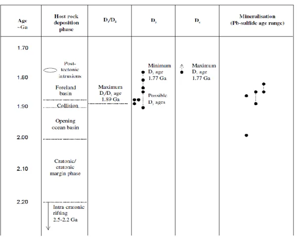
Regarding the evolution described in the previous section, three main ductile deformation patterns, D1 - D3, exist in Central Lapland (Hölttä et al., 2007). Apart from these three main deformation patterns there is a brittle deformation pattern, D4, dated to about 1.77 Ga which includes numerous discontinuous and low displacements brittle shear zones (Patison et al., 2007).

Figure ‎2.1: Main geologic units of northern Finland. Pe: Peräpohja schist belt, Ku: Kuusamo schist belt, So: Sodankylä schist area, Sa: Salla greenstone area, Ki: Kittilä greenstone area (Hanski, 2005).

D1 and D2 are related to the oldest mapped deformation fractures due to thrusting at the CLGB margins, one with N to NE direction at the southern margin and the other related to S to SW directed thrusting at the northern margin, emplacing of the Lapland Granulite Belt

(19)

9

over the N and NE margins (Fig. 2.3); all these are known as major thrust events of D1/D2. (Patison, 2007)

Figure ‎2.2: Main lithostratigraphic units of central Finnish Lapland (after Räsänen et al., 1995). The study area indicated with red rectangular.

The Sirkka line (Shear zone), resulted from convergence at the southern margine of CLGB, is the main rheological boundary within the CLGB which separates the sediment-dominated rocks of the Savukoski Group in the south from the volcanic-sediment-dominated package

(20)

10

of the Kittilä Group in the north (Patison, 2007). The D3 deformation denotes strike-slip shear zones such as the Kistala Shear Zone that intersects D1/D2 thrust zones. Ward et al., suggested that the movements on D3 produced a dextral rotation of the maximum principle stress (δ1)of the entire CLGB. A summary of the main deformation events and related dates are shown in Table 2.2.

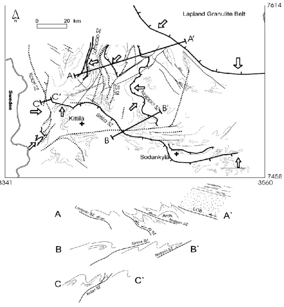
Figure ‎2.3: Tectonic map of the Central Lapland Granitoid Complex. Arrows show the interpreted tectonic transport directions. Thick solid lines with ticks are thrusts, dashed thick lines are steep shear zones and solid medium lines are late faults. Ki SZ = Kiistala Shear Zone, SZ = Shear Zone, LGB: Lapland Granulite Belt. Below the map, schematic vertical sections along lines A-A’, B-B’ and C-C’ (Hölttä et al., 2007).

(21)

11

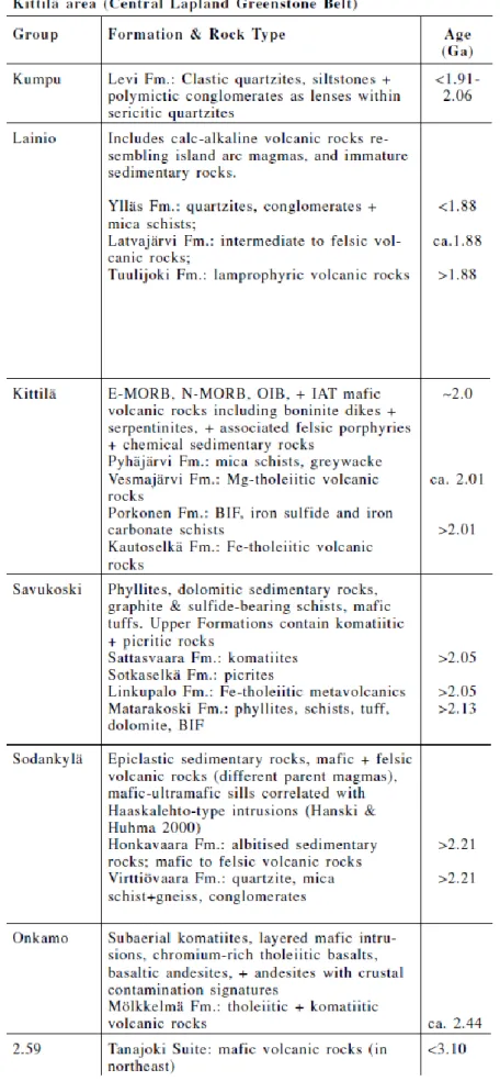
Figure ‎2.4: Stratigraphy of the Central Lapland greenstone belt and their approximate ages, after Hanski et al., 2001.

The Suurikuusikko gold deposit with more than 2 million ounces and a depth extension to at least 500 m is known as the largest gold resource in northern Finland; it occurs within rocks of the Kittilä Group. The Suurikuusikko mineralization with an approximate age of 1.89-1.85 Ga occurs on D3 shear zones within a mostly N-striking segment of the otherwise generally NE-striking direction (the Kiistala Shear Zone). (Patison et al., 2007)

(22)

12

Table ‎2.1: Summary of stratigraphy of the Central Lapland greenstone belt and rock types. Fm= formation, (Patison et al., 2006).

(23)

13

2.2. Postglacial rebound

Loading and unloading of the ice sheets cause various changes in the physical conditions of the influenced region such as: changes in vertical load, crustal strain, crustal deformation and seismicity.

In order to have a better understanding of the crustal behavior during the loading and unloading periods of ice sheets, several postglacial rebound models have been produced during the last decades (James and Morgan, 1990; Spada et al., 1991; James and Bent, 1994; Wu and Hasegawa, 1996a, b; Wu, 1996, 1997; Johnston et al., 1998; Klemman and Wolf, 1998; Wu et al., 1999).

Table ‎2.2: Summary of available dates and timing relationships between CLGB deposition, deformation, metamorphic, and mineralizing events. Plotted date ranges include error bars (Patison et al., 2007).

In the late stages of deglaciation, the vertical stresses are reduced; therefore, the elastic rebound causes crustal uplift, faulting and seismicity (Fig. 2.5) (Stewart et al, 2000). The uplift was very fast after deglaciation and slowed down quickly to the present state with a maximum uplift of about 9 mm/year (Kuivamäki et al., 1998). However, postglacial

(24)

14

rebound models are not unique and they cannot explain the lateral variations in the rheological structures (Davis et al., 1999).

2.3. Postglacial faults in Fennoscandia

In northern Fennoscandia, the postglacial (PG) or late-glacial faults are the results of the unloading of the ice during the last Weichselian glaciation (~9 000 to 10 000 years B.P.) (Lagerbäck, 1990).

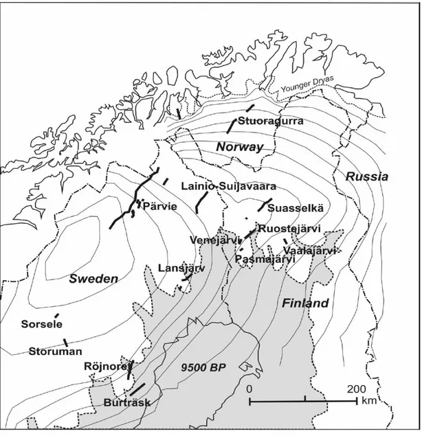
There are at least 14 known locations in Fennoscandia where PG faults can be seen, with lengths of 2 to 160 km and maximum surface displacement of up to 30 m (Fig. 2.6 & Table 2.3), (Olesen et al., 2004; Lagerbäck & Sundh, 2008).

The PG faults in Fennoscandia mostly strike in the SW-NE direction and dip to SE; these are mostly reverse faults with dip angles between 30-60 degrees at the surface, and are located in old, reactivated fracture zones (Munier & Fenton, 2004). Experiments on hydraulic properties of the PG faults illustrate that most of the PG faults in the uppermost bedrock are connected with an increase in hydraulic conductivity (Kuivamäki et al., 1998).

Considering the landslide distribution and dimensions of the PG faults, the magnitude of the paleo-earthquakes that formed the PG faults is estimated to have been between M5.1 and M7.5. The distribution of recent earthquake epicenters is mainly located on the SE-sides of the PG-fault lines which indicates the dip towards SE.

Moreover, it has been discovered that most of the large PG faults in northern Fennoscandia are cutting Quaternary deposits; however, no faults are found in the central and southern Finland cutting Quaternary soil layers. The PG faults in northern Finland mainly strike from NE-SW to NNE-SSW with the SE side of the faults uplifted. (Kuivamäki et al., 1998)

2.4. Suasselkä PG-fault

The Suasselkä PG-fault (earlier known as the Rautuskylä fault (Kujansuu, 1964)) is classified as a late-glacial thrust fault; its length has a minimum of 36 km and a maximum of 70 km (including the SW extension). The Suasselkä PG-fault is situated in the middle of the Kittilä greenstone area, with a strike direction which varies between 35o-50o and a maximum scarp height of 5 m (Kuivamäki et al., 1998). Studies show that the Suasselkä PG-fault follows an old major shear zone (Kuivamäki et al., 1998) striking in NE-SW direction with a length of tens of kilometers and a width between 1 to 1.5 km (Fig. 2.7) (Kuivamäki et al.,

(25)

15

1998). An electromagnetic study carried out by Paananen et al. (1987) shows that the fault is dipping toward the SE. The surface trace of the fault cuts the CMP line 2 of HIRE V2 profile at about CMP 3700 (Fig. 4.1)

Figure ‎2.5: An illustration of the impact of glacial loading (a) and unloading (b) on the crust in a region with a compressive stress regime (Stewart et al, 2000).

(26)

16

Figure ‎2.6: Distribution of PG faults in northern Fennoscandia (thick lines); adapted from Kukkonen et al., 2010.

Table ‎2.3: Summary of PG faults within the Lapland Fault Province and their characteristics (Stewart et al, 2000).

(27)

17

Figure ‎2.7: Location of Suasselkä PG fault in the Kuoko area and the old shear zone (Härkönen et al., 1989).

3. Review of the seismic reflection method

Seismic techniques, including the seismic reflection method, have improved during the last years and they are one of the most important geophysical methods with a large number of geophysicists involved. The most important advantages of seismic methods compared to other methods are the accuracy, high resolution and ability of great penetration (Sheriff, 1995). In a seismic experiment, the seismic waves propagating from a controlled source interact with subsurface targets that reflect, refract and diffract. The reflected, refracted and diffracted waves can be detected by the seismometers located on the Earth’s surface; the result obtained after processing of these waves, is an image of the surface targets. (Scales 1997)

Depending on whether data acquisition is on land or in marine environments, two types of receivers (sensors) can be used, Geophone and Hydrophone. A magnet and coil are the main components of a geophone; the motion of the magnet generates a voltage which is proportional to the velocity of the Earth.

(28)

18

In order to increase the signal to noise ratio and also attenuate horizontally propagating waves, the signals in each receiver is summed. Ground roll is horizontally-propagating Rayleigh waves that can mask the reflection events. Low frequency, high amplitude and low group velocity are ground roll characteristics.

The seismic energy can be generated by different kinds of seismic sources depending on the type of survey (on land or marine) and also the types of targets; both compression and shear energy can be generated by a vibrator source depending on the type of the vibrator.

A trace is the time-series recorded by each receiver. Four main configurations of the source receiver gathers of the traces are available: common midpoint gather, common receiver gather, common shot gather and common offset gather. The geometry of the recording and the ray paths related to these main methods are shown in Fig. 3.1.

Figure ‎3.1: (a): Stacking chart, each dot represents seismic trace. (s,g) shot-geophone and (y,h) are the midpoint-offset coordinates. (b): (1) a common-shot gather, (2) a common-receiver gather, (3) a CMP gather and (4) a common-offset section. Solid triangles represent receiver positions and solid circles denote shot locations, x is the cable length, E denotes a midpoint and E’ denotes a depth point (Yilmaz, 2001).

(29)

19

3.1. Seismic wave equation

Assuming the Earth is an isotropic solid, the stresses and strains can be calculated. In the first step, the stresses to strains are related by using Hooke’s law. However, since seismic waves are time-dependent the momentum equation should be utilized as well.

3.1.1. Hooke’s‎law

The strains involving seismic wave propagation, except in the areas where they are very close to the source, are usually small. This makes it possible to use Hooke’s law to relate the seismic stress and strain, the tensor expression of Hooke’s law can be written as (Shearer, 1999):

where is a fourth order elastic tensor, by assuming that the elastic tensor is invariant with respect to rotation, it can be written: :

where (shear modulus) and are the Lamé parameters of the material and is the Kronecker delta, by inserting equation (2) into (1) it can be written:

In addition to the Lamé parameters, there are other common elastic constants (Shearer, 1999): Young’s modulus: Bulk modulus: Poisson’s ratio

(30)

20 P-wave velocity:

S wave velocity:

where ρ is the density.

3.1.2. Momentum equation

Assuming x is the particle’s position in the undisturbed Earth’s equilibrium state, the particle motion after a small disturbance of the Earth is given by:

where u is the displacement

therefore, the equation of the motion (i.e. momentum equation) can be written as: where:

: Earth’s equilibrium density,

: equilibrium gravitational potential field,

: equilibrium pressure field which (i.e. I is the unit vector) is equal to the purely hydrostatic equilibrium stress field ,

and , and are the “incremental” quantities regarding the time-dependent stress,

density and gravitational potential at the particles new position (r)(Scales, 1997).

After calculating the incremental quantities the momentum equation (10) can be written as:

Where, is the increment which is added to the initial stress at the particle x ( ) to

calculate the total stress; since the stress tensor at a particle is known, the stress tensor at a point in space ( ) can be defined by:

(31)

21

Equation (11) is the full equation of the motion including the gravitational term. In terms of seismic waves where one is dealing with high frequencies, the gravitational term can be ignored; therefore, the elastic term is the only remaining part and the equation (11) breaks down to:

where:

By substituting equation (14) into (13) the elastic wave equation can be written as:

By taking the divergence and curl of equation (15), and use of the Helmholtz decomposition theorem to express the displacement vector as: , where A and are the S-wave vector potential and P-S-wave scalar potential respectively, and considering the vector identities and , the wave equations for P and S waves can be calculated separately (Shearer, 1999).

By taking divergence of the equation (15), the equation below is obtained (equation 16):

where the P-wave velocity, , is given by

and by taking curl of the equation (15), equation 18 is obtained as:

where the S-wave velocity, , is given by

(32)

22

3.2. Snell’s‎law

Whenever the elastic properties of a media change such as at a surface separating two units, the energy of the wave encountering the separating surface partly will be reflected and remain in the same medium and partly will be refracted into the other medium with a change in the direction of propagation. Refraction and reflection are the basics in exploration seismology.

Consider a plane wave-front AB incident on an interface as in Fig. 3.2 According to the geometry in Fig. 3.2 the below is obtained:

and hence

where angle is called the angle of incidence, is the angle of refraction and equation (22) is known as Snell’s law. (Sheriff, 1995)

Figure ‎3.2: Reflection and refraction of a plane wave (Sheriff, 1995).

3.3. Partitioning at an interface

The partitioning of energy at an interface between two media and how the wave energy is divided into transmitted and reflected energies are important factors in seismic

(33)

23

exploration; the normal incidence case is a simple case which is commonly assumed in the seismic reflection method.

Consider an incident P-wave on an interface between two media with different velocities (Fig. 3.3); in this case, the Zoeprritz’ equations reduce to very simple equations. (Sheriff, 1995)

The acoustic impedance (Z) is defined as:

where ρ is the density of rock and v is the wave velocity.

The total energy of the transmitted and reflected rays is equal to the energy of the incident ray, therefore:

Figure ‎3.3: Generated waves at a solid-solid interface by an incident P-wave (Sheriff, 1995).

and

hence for the reflection coefficient R, the below can be written :

where , , and , , are density, P-wave velocity and acoustic impedance for the upper(1) and lower(2) layers respectively, the reflection coefficient varies between -1 and 1.

(34)

24 The transmission coefficient, T, can be written as:

3.4. Fresnel Zone

A reflection is the returning energy that comes from a large area of a reflector; the area that the reflected energy arrives at a detector within half a wavelength represents the Fresnel zone. Since the major portion of seismic signal comes from the first Fresnel zone it is known as the horizontal resolution of the seismic data (Sheriff, 1995). The first Fresnel zone for a reflector located at depth h0 can be written as:

where t is arrival time, is average velocity and is the frequency. The effective Fresnel zone is known as:

3.5. Zero-offset

Huygens’ principal allows us to consider the reflections as the summation of point sources along a reflector. This in turn simplifies the problems regarding wave propagation and enables picturing a reflection event (Scales, 1995).

The Zero-offset travel-time section is an important concept in which the receiver and the source are placed together at the surface (Fig. 3.4). By moving the source-receiver pair along the profile above a reflector and repeating the experiment and plotting the results, the Zero-offset travel-time section will be provided. The fact that more than one wave arriving with the same time as the source-receiver pair passes the syncline makes the travel-time curve to be multi-valued and shaped as a “bow-tie” (Fig. 3.5). One of the migration tasks is to solve this problem and the result of migration will be the correct travel-time curve (section 3.9). (Shearer, 1999)

(35)

25

Figure ‎3.4: Illustration of down going seismic waves in zero-offset case (Shearer, 1999).

Figure ‎3.5: (a) A syncline reflecting interface and (b) corresponding unmigrated “bow-tie” shape travel-time curve (Kearey, et al., 2002).

In practice there is an offset between source and receiver; and the travel-times are the function of offsets (e.g. the CMP case). In order to have the zero-offset travel-time section the time difference between the zero-offset case and the finite-offset case has to be corrected (NMO correction).

(36)

26

3.6. Reflection paths

3.6.1. Horizontal reflector: Normal move out

A horizontal reflector is the simplest case in the 2D reflection problem, in where the dip is zero (Fig.3.6). The difference in time of arriving waves which is a result of the difference in the offset between source and receiver is known as normal move-out (NMO):

where x is the offset, v is the average velocity and h is depth of the horizontal reflecting bed.

Figure ‎3.6: Geometry of a reflected ray path (top) and corresponding travel-time curve as a function of source-receiver offset (bottom), for a constant velocity travel-times form a hyperbola (Shearer, 1999).

3.6.2. Dipping reflector: dip move out

When the interface between two media is not horizontal to the direction of the profile, another correction has to be taken into consideration, the correction known as DMO.

DMO correction migrate each trace to zero-offset, therefore, the DMO corrected data is identical to the zero-offset section (Fig. 3.7) (Deregowski, 1986).

(37)

27

Figure ‎3.7: Reflector point dispersal ( ) increases as the square of the offset (h) and is inversely proportional

to the traveltime (D) (Deregowski, 1986).

The time, t, takes for a reflected ray from source to receiver in the case of a dipping reflector with a dip equal to θ and distance between receiver and source (offset) equal to h with average velocity equal to v for the medium above the reflector is:

The NMO velocity for the dipping reflector can be written as:

From the above equation it is obvious that the velocity for a dipping reflector is always greater than the medium velocity. In addition, the true dip of the reflector is always greater than the apparent dip (Fig. 3.7).

Figure ‎3.8: Illustration of the apparent dip in the dipping reflector case and its true dip after migration (Scales, 1997).

(38)

28

3.7. Common-midpoint method

Common-midpoint (CMP) seismic acquisition is a multifold method, in which traces related to a specific midpoint are used to form a CMP gather. After applying NMO and DMO corrections and summing all the traces for each midpoint, a CMP stack is obtained along the entire profile.

The number of source and receiver pairs (ng) for one midpoint which is known as CMP fold

coverage, (nf), is given by:

where ∆g is the receiver-group interval and ∆s is shot interval (Yilmaz, 2001). An example of a six fold common midpoint gather can be seen in Fig. 3.8.

Figure ‎3.9: Six fold CMP gather. S: source locations, G: receiver locations (Yilmaz, 2001).

3.8. Deconvolution

Considering we oversimplify the modification of the wave during its passage through the earth in the way that the recorded data on a seismogram is composed of the earth’s impulse response, random noise and the input wavelet. The process that compresses the input wavelet and removes the short-period multiples is called deconvolution and the result from deconvolution is the seismic trace including only subsurface reflectivity. Therefore deconvolution increases the temporal resolution.

Mathematically, the convolution model in the time domain for a noise-free seismogram can be written as:

(39)

29

where x(t) is the recorded seismogram, w(t) is the input wavelet, e(t) is the earth’s impulse response and * represents convolution.

In the frequency domain the convolution model can be written as:

where , and are the spectra of x(t), w(t) and e(t), respectively.

Since the earth acts as a filter of seismic energy, to solve the convolution problem we start by introducing a filter operator in the way that:

Therefore:

where is the Kronecker delta.

In other words, the filter operator is the inverse of the seismic wavelet w(t). (Yilmaz, 2001) The main objective of deconvolution is to extract the reflectivity function from the seismic trace. The only known in equation (34) is x(t); therefore, in order to overcome the problem some additional assumptions have to be made. The most common one is that the seismic wavelet is a minimum-phase. One solution to equation (34) is the least square filter or Wiener filter in which the determined filter gives minimum error between the actual and desired outputs in the least-square sense.

Consider the input data, , and the filter that has to be determined, , and the output set to be . The error between the actual and desired outputs is: .

The least square method can be written as:

where is the partial derivation with respect to elements of ( ).

The equation (38) can be written using the definition of cross-correlation and autocorrelation as:

(40)

30

where is the autocorrelation of , is the cross-correlation of and , and j =

t-k .

Equation (39) is known as normal equations which are used to perform spiking deconvolution.

Another assumption is that the earth’s impulse response, , has a flat (white) spectrum (at least over some limit band pass); in addition the fact that is causal, enables simplifying the normal equations to the spiking deconvolution or whitening case.

In frequency domain the whitening is equal to finding an inverse filter whose transform is , where:

is the frequency and is the transform of the input.

In order to avoid frequencies that are related to noise, the whitening has to be performed only over a limited band pass. (Sheriff, et al., 1995)

3.9. Migration

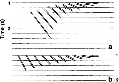
The unmigrated recorded travel-time curves are oriented with respect to the observation points (Sheriff, et al., 1995). The purpose of migration is to move the reflections into their true spatial position; this involves re-positioning of reflections (e.g. dipping reflections) or diffracting points.

In the dipping reflector case, the reflections on the migrated zero offset section are steepened, shortened and moved in the up dip direction.An example of migrated and unmigrated zero-offset sections for different dipping reflectors is shown in Fig. 3.9. As mentioned in the section related to zero-offset the “bow-tie” is the result of an unmigrated travel-time over a syncline or anticline reflecting interfaces, Fig. 3.10 shows syncline and anticline features and corresponding migrated zero-offset sections, note the up dip movement of dipping segments A, B, D and E in the migrated section while the horizontal segment C is remains unchanged. (Yilmaz, 2001)

(41)

31

Figure ‎3.10: Zero-offset sections modeled for reflectors with different dipping angles before (a) and after (b) migration (Yilmaz, 2001).

Figure ‎3.11: Travel-time curves recorded for different syncline and anticlines before (a) and after (b) migration (Yilmaz, 2001).

(42)

32

3.9.1. Finite- Difference (FD) migration

Finite difference time domain migration is one of the most widely used migration methods and uses the downward continuation of the seismic wave-field principle. Provided that the wave-field is known at the surface of the earth, it can be continuously traced downward to the reflectors by increasing the depth of the receivers with finite steps. As shown in Fig. 3.11 by moving the receiver line downward, the diffraction hyperbola is collapsing to a point.

Figure ‎3.12: By moving the receiver line while decreasing its length, the diffraction hyperbola breakdowns to a point (Sheriff, et al., 1995).

Mathematically, the finite difference time migration is the finite-difference solution of the parabolic wave equation (eq.43).

A vertically down-going plane wave is defined as:

where Q(x,z) is not constant but varies slowly. By substituting equation (41) into the scalar wave equation ( ) it can be expressed in terms of Q as:

for a wave-field close to vertically propagating plane wave (“15o approximation”), equation (42) is drop to:

(43)

33

3.10. Crooked line method

Due to several structural or environmental difficulties, sometimes it is impossible to locate the seismic profile along a straight line; therefore, the line has to be bent in some areas. The survey method utilized in such cases is called the crooked line method.

In order to apply normal move-outs and also calculate the correct midpoints, the correct distance between source and receiver has to be calculated. Since a spread in midpoints exist, it is common to consider a best-fitting straight line trough the midpoints; and construct perpendicular bins to organize the midpoints in the way that all the traces whose midpoints fall in a bin stack together (Fig. 3.13). (Sheriff, et al., 1995)

Figure ‎3.13: An exaggerated schematic of 2D crooked line profiling (Nedimovic and West, 2003).

4. Acquisition parameters

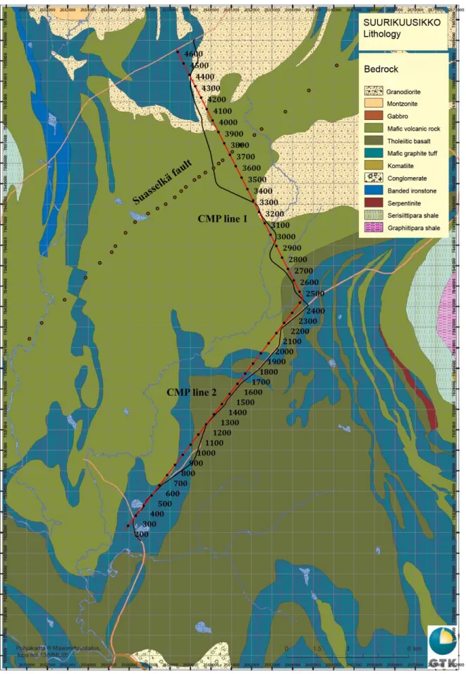
The seismic profile which is processed in this study (line V2) is the easternmost line presented in a previous seismic reflection survey in the Suurikuusikko gold mining and exploration area located in Kittilä north of Finland. The survey was done in the period of February to March 2008. The project was a part of the High Resolution Reflection for Ore Exploration (HIRE) started in 2007. The survey is a 2-D reflection survey and the lines are chosen with regards to roads and geology specifications of the area. The V2 line with a total length of 30675 m runs from south to north. In the south it passes mafic graphitic tuffic rocks, which are buried under a layer of tholeiite in the middle of the line (Fig. 4.1).

(44)

34

The difference between the highest (in the north) and lowest (in the south) points of the profile is about 70 meters. The common-midpoint (CMP) method has been used in the processing and asymmetric shooting were carried out at the ends of the line (Kukkonen et al., 2009). The shooting interval varies from 25 to 50 meters depending on the local geological and structural conditions. A 15.4 ton Geosvip was used as the source. The data were recorded in SEG-Y format (Kukkonen et al. 2009).

The positioning of the lines was carried out using GPS, and a 25 m steel rope before acquisition. Horizontal positioning was carried out with use of differential GPS to an accuracy of at least ±2 m, and leveling was calculated to an accuracy of at least ±0.5 m (Kukkonen et al. 2009).

The data acquisition parameters for line V2 can be seen in Table 4.1

Table ‎4.1: Acquisition parameters for HIRE reflection seismic live V2 (Kukkonen et al. 2009).

Parameter Detail

Number of channels Sampling interval

Record length after correlation Number of sweeps/source Sweep frequency Geophone spacing Source spacing Source type Tape format Stacking fold Acquisition geometry Medium type Profile length

Number of source points Number of receivers 402 1 ms 6 s 6 30-165 Hz 12.5 m 25 or 50 m Vibroseis SEG-Y Varying

Symmetrical, split spread Hard

30675 m 832 2537

(45)

35

Figure ‎4.1: The position of the HIRE line V2, the CMP lines (in red) and surface trace of the Suasselkä PG fault.

(46)

36

5. Data processing

The on-site data processing was accomplished by VNIIGeofizika (All-Russian Research Institute of Exploration Geophysics) at the field base (Kukkonen et al. 2009). In the next stage the collected data for line V2 was processed in this study using the following steps (Table 5.1):

Table ‎5.1: Processing steps used in this study.

Processing steps for the reflection seismic data 1. 2. 3. 4. 5. 6. 7. 8. 9. 10. 11. 12. 13. 14. 15. 16. 17. 18. 19.

Read SEG-Y format data files

Create geometry data base (including two separate CMP straight lines) Apply geometry

Picking first arrivals

Trace editing (noisy and dead traces were killed) Refraction statics:

Seismic reference datum: 280, replacement velocity: 5700 m/s, weathering layer velocity: 1750 m/s Zero-phase spectral equalization: band-pass filter region: 25-40-140-160 Hz

Time-variant band-pass filtering: 0-500 ms: 40-60-140-200 Hz 1000-1500 ms: 35-55-130-180 Hz 2000-3000 ms: 30-45-120-160 Hz 4000-6000 ms: 25-40-120-160 Hz AGC: window length: 200 ms

Re-sample: sample rate: 1 ms, trace length: 3000 ms Velocity analysis

NMO correction: 40% stretch mute Residual statics:

Surface-consistent, time-window length: 500-2800 ms DMO correction:

CMP spacing: 6.25 m

Number of offsets processed at a time: 4 Velocity analysis

Stack

Post-stack coherency filtering Migration:

Finite-Difference migration (FDMIG), using smoothed NMO velocities Depth conversion

(47)

37

5.1. Apply geometry

The geometry information of the shots and receivers was added to the shot gathered data; in order to have both a proper fold and also offset distribution (i.e. each bin includes an even fold and offset distribution) in all CMP bins. CMP bins were arranged along two straight lines with CMP spacing of 6.25 m; a total number of 4455 bins was established. The CMP information inserted to the trace headers.

5.2. Elevation and weathering static corrections

The differences in shot and receiver elevations can cause shifts in reflection events; therefore, it is necessary to correct for surface irregularities. Elevation correction was carried out using a datum level of 280 m with a replacement velocity of 5700 m/s. First break picking was done both automatically and manually on shot gathered data in the offset range of 0 to 4700 m. The best fitting two layered model consisted of about a 17 m average thick weathering layer with a velocity of 1750 m/s, and a RMS misfit equal to 4.8 ms. Furthermore, based on this model, refraction statics were calculated and applied. The refraction statics remarkably influenced the improvement of the data, a good shot gather example with and without static corrections is shown in Fig. 5.1.

5.3. Trace editing, filter, zero-phase spectral equalization, muting and re-sample

Trace editing was carried out by killing dead and noisy traces. The decrease in the amplitude and increase in the wavelength of the seismic wave with time while it is passing through the earth due to geometrical spreading, and also existence of some low-frequency noise such as ground roll, and also some high frequency ambient noise all support the use of a suitable frequency filter.

(48)

38

Figure ‎5.1: A shot gather showing the effect of the refraction static correction (the horizontal axis is the receivers’ position).

Regarding processing of seismic data, band-pass filtering is one of the most commonly used and effective filters. Having tested several various filters, the best result was achieved by applying a time-variant band pass filter. Not only the time-variant filter caused deeper reflectivity of steeply reflections to be emphasized, but also it reduced the noise in the earlier parts of the records. An example of a shot gather before and after filtering is shown in Fig. 5.2. In order to increase the temporal resolution zero-phase, spectral equalization with a window length of 30 Hz was applied to flatten the amplitude spectrum (Yilmaz 2001). Regarding the muting of the first breaks, the stacked sections with and without muting the first arrivals have been compared; in order to include all the reflection events, especially in the upper parts, no first break muting was applied. Traces were re-sampled at 1 ms down to 3000 ms.

(49)

39

Figure ‎5.2: A shot gather showing the effect of the filter, note the steeply dipping reflection after applying the filter (the horizontal axis is the receivers’ position).

5.4. Velocity analysis and residual statics

Apart from the corrections for elevation and the weathering layer, surface irregularities such as irregular near-surface weathering layer, can cause changes in reflected traveltimes; therefore residual static correction is a significant step in seismic processing. After sorting the data into CMPs, velocity analysis was performed in order to calculate the residual statics and the first proper NMO velocity was obtained for each CMP line (lines 1&2). The resulting NMO velocities have been used to produce the move-out corrected CMP gathers for each CMP line. The surface-consistent residual statics consisted of 8 iterations calculated for the NMO corrected CMP gathered data. The best calculated residual static result among the 8 iterations was applied to the CMP gathered data. In the next step, in order to improve the NMO velocities a second velocity analysis was carried out and the process repeated. Since there was no significant improvement observed in the third attempt, the process was stopped after the second iteration.

(50)

40

5.5. Dip Move Out (DMO) correction

Regarding the DMO velocity formula (formula 32), the velocity for steeply dipping reflections will be higher than the true velocities; this is a significant issue especially in the case of the crystalline environment where several steeply dipping reflections are in the vicinity of gently dipping ones; therefore, in order to have a stacked section with both gently and steeply dipping reflections with the same strength and also a section that is equivalent to the zero-offset section (see section 3.6.2), it is necessary to correct the effects of the dip. The DMO process begins with sorting the data into common offsets. With respect to the fold coverage and offset ranges, the most optimal offset range was -2500 m to 2500 m with an interval of 10m and a bin size equal to 5 m were chosen and the DMO correction was applied after correcting for NMO. The DMO corrected stack section showed significant improvement and the NMO velocities were considerably smoother and more uniform (ca. 5200-6500 m/s) compared with the velocities before the DMO correction (ca. 4900-8200 m/s). In addition, both gently and steeply dipping reflection events were stronger. For comparison, a selected portion of the stacked sections before and after DMO corrections are shown in Fig. 5.3.

5.6. Time migration

One important goal in a seismic reflection experiment is to search for the relation between the seismic image and the geological and structural features in the study area. The goals and the importance of migration have been described previously. Thus, it is important to search for the most appropriate migration algorithm that gives the best possible result. After testing different migration algorithms, the most reliable result was achieved using Finite Difference (FD) migration. Following testing different migration velocities including the varying smoothed NMO velocity, the relatively best result was obtained using a NMO smoothed velocities. Due to the sharp change in direction of the CMP lines in the middle of the profile (CMP 2440), the migration was carried out separately for each line in order to have a proper image of the reflectors and their correct positions and dip directions (for steeply dipping reflectors).

(51)

41

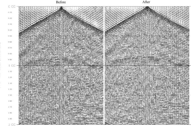
Figure ‎5.3: Stacked sections (CMP 3200-4623) before (A) and after (B) DMO correction, note the presence of sub-horizontal reflections together with steeply dipping reflections with same strength (arrows) and movement of the reflections to their zero-offset position in (B).

B

A

(52)

42

6. Stacked and migrated sections

Regardless of the good acquisition parameters, because of the crooked geometry of line V2 and also various geological and structural discontinuities (e.g. Suasselkä fault) in the area, choosing the most effective CMP line was a challenging problem; many configurations of the CMP lines were tested, the relatively best result was obtained in the case of two separate straight lines (Fig. 4.1). Although there is a significant difference between the direction of the CMP lines at the intersection point (CMP 2440), the characteristics of the reflection events are consistent in both the migrated and unmigrated sections. The time migrated and unmigrated sections for each CMP line can be seen in Fig. 6.1 and 6.2.

(53)

43

Figure ‎6.1: Unmigrated stacked sections for CMP line 1 and 2 (see Fig.4.1 for location of the CMP lines). CMP line 1

(54)

44

Figure ‎6.2: Time-migrated stacked sections for CMP line 1 and 2(see Fig.4.1 for location of the CMP lines). CMP line 2

(55)

45

7. Comparison with previous work

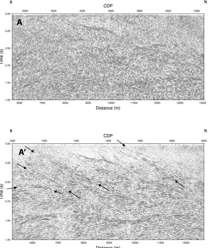
Good acquisition parameters such as high fold coverage and short source and receiver spacing enabled obtaining improved signal strength after stacking. Moreover, each processing step was carried out carefully by testing the effect of several parameters and selection of the most appropriate result for each step. This allowed improving the signal to noise ratio in both the migrated and unmigrated sections. The migration worked very well, in correcting for both the dipping events and diffraction events generated by point reflectors; therefore, it has increased the resolution. The selections of two straight CMP lines provided an even offset and fold distributions in each CMP bin. Moreover, the resulting stack section without muting was very well detailed. The stacked unmigrated sections are compared with previously processed sections (Fig. 7.1).

Regardless of the prominent appearance of reflectivity in all parts, several reflection events were observed at both lower and higher times; furthermore, the continuity of the reflection events, especially in the case of the reflections reaching the surface, is more obvious. The DMO application assisted enhancing both steeply and gently dipping reflectors with the same strength. Some of the most prominent improvements are shown in Figures 7.2, 7.3 and 7.4.

(56)

46 F ig ur e ‎7 .1 : Th e u n mig ra ted s ta ck ed s ec tio n s to p : p rev io u sly p ro ce ss ed , b o tto m: r e -p ro ce ss ed .

(57)

47

Figure ‎7.2: Stacked sections A and A’ (based on Fig. 7.1). Note the appearance of several reflections (the arrows).

(58)

48

Figure ‎7.3: Stacked sections B and B’. Note the improved signal to noise ratio in B’ compared to B (based on Fig. 7.1).

(59)

49

(60)

50

8. Interpretation

The software, GoCad, was used for 3D illustration of the seismic lines and correlation with surface geology (Fig 8.1). Based on the different reflection characteristics in the migrated seismic section, four main seismic units can be identified, marked as, A, B, C and D (Fig. 8.2 & 8.3). Several reflections, including steeply dipping and sub-horizontal reflections (R1, W1, F1, F2 and M1), are present in the migrated seismic section (Fig. 8.2 & 8.3).

8.1. Geological interpretation

The aim of the Geological interpretation is to search for the geological meaning of the seismic data. The migrated seismic sections have been interpreted using the information from the surface geological map, airborne magnetics and the surface trace of the Suasselkä PG fault. The prominent reflection events correlate well with the surface geology. The contrast in acoustic impedance between mafic graphitic tuff and tholeiitic basalt rock units produces very strong reflections (i.e. R1) that can be traced well up to the surface. The contrast between the mafic volcanic and tholeiitic basalt rock units appears to be less strong with relatively weaker reflection events (W1). The airborne magnetic map shows a considerably higher magnetic contrast between the granodiorite and the mafic volcanic rocks, however, this boundary appears to be seismically transparent.

(F1) most probably represents the detachment level which separates other overlying units from the relatively weak reflective unit (A), with a varying depth from about 3 km in the north down to about 4 km in the south. The highly reflective unit (B) with an extension of about 3 km depth in the CMP range 1100-1900 correlates with the tholeiitic basalt rock unit. In the beginning of the profile, up to about CMP 1100, unit (C) correlates with the mafic graphitic tuff, it seems that its extension to more than 4 km is the deepest among the overlaying units. In the north, from about CMP 3100, the highly reflective unit (D) most probably represents the youngest rock units among others (granodiorite) down to a depth of about 3 km.

8.2. Structural interpretation

In the northern part of the profile, in the vicinity of the Suasselkä PG fault, there is a good correlation between its surface trace (about CMP 3700) and the moderately dipping reflection (F2).

(61)

51

The fault can be traced down to approximately 3 km depth with a dip direction towards the SE. The dip varies between 35o to 50o (the dip decreases with depth). Most probably the fault (F2) truncates against the décollement zone (A). The existence of the Suasselkä thrust fault together with the nicely imaged reflection packages of M1 and also the direction of the thrust, suggest a thrust duplex structure, which formed a décollement zone. It is most likely that relatively high reflective unit (D) has been thrusted into the system over the base unit (A) at a later stage. The dip direction of the major structure in the northern parts, especially along CMP line 1, is towards the NE.

(62)

52 F ig ur e ‎8 .1 : 3 D illu str a tio n o f th e seismic lin es a n d th e su rfa ce g eo lo g y ma p . CM P l in e 1 CM P lin e 2

(63)