A simple structural index based on FWD measurement

VTI särtryck

Nr 223 ' 1994

A Simple Structural Index Based

on FWD Measurement

Håkan Jansson

Paper presented at the 4th International Conference

on the Bearing Capacity of Roads and Airfields,

July 17 21, 1994, Radisson South Hotel, Minneapolis,

Minnesota, USA

Väg- och

V'" särtryck

Nr 223 0 1994

A Simple Structural Index Based

on FWD Measurement

Håkan Jansson

Paper presented at the 4th International Conference

on the Bearing Capacity of Roads and Airfields,

July 17 21, 1994, Radisson South Hotel, Minneapolis,

Minnesota, USA

db

Väg- och

transport-farskningsinstitutet

'

ISSN 1102 626X

A SIMPLE STRUCTURAL INDEX BASED ON FWD MEASUREMENT Håkan Jansson

Swedish Road and Transport Research Institute (VTI), Sweden

ABSTRACT

Results from Falling Weight De ectometer (FWD) measurements are often used in a backcalculation program in order to determine layer moduli. Stresses and strains in the pavement can then also be determined. In this paper, simple algorithms are presented, which calculate the horizontal strain in the bottom of the asphalt layer directly from the measured de ections without the need for any additional data. The layer thicknesses are not included as in practice they vary more or less from one section to another. Different algorithms for the most commonly used positions of the sensors on the FWD are

developed from linear elastic analysis of a wide range of Swedish pavements. The

estimated asphalt strain may be used as an indication of the structural strength of the pavement, regardless of whether it is cracked or not. If the number 1000 is divided by the asphalt strain, in microstrain, the result is most often a value between 1 and 10. This may be a structural index and is a fast and easy way of expressing the structural condition of the pavement.

INTRODUCTION

Nondestructive testing to determine the structural condition of pavements has been performed for a considerable number of years. The equipment used in Sweden, as in

many other countries, is the FWD. The reason for measurement and also the way in

which the results are interpreted may vary. A common way of analysing the results is to determine the elastic moduli for different layers in the pavement as well as for the subgrade. This requires layer thicknesses and Poisson's ratios to be known for the layers. In recent years, programs have been developed that are more user friendly and superior in some respects. The calculations are also made much faster today. Some of the

problems involved with backcalculations are, however, still the same. It is sometimes

difficult to find realistic moduli, especially if the pavement is complex. Should there be a stiff layer or not, and if so at what depth? (The MODULUS program has a convenient

solution to this [l]). Does a variation in calculated modulus along a road re ect a

variation in material stiffness rather than a variation in layer thickness? The fact that layer thicknesses vary in practice is well known and this will affect the calculated moduli. This is especially true for a thin, stiff layer, e.g. a thin asphalt concrete layer. (Other problems concerning the fact that the materials are not homogeneous or linear elastic are not addressed here). Often, the moduli themselves are not of primary interest, but rather the pavement performance and the stresses and strains in the pavement.

Algorithms for estimation of strain in the asphalt layer directly from the surface de ections were developed by Thompson and Hoffman [2]. The concept was adopted in the mid 19805 in the development of a Swedish overlay design procedure based on FWD measurements. Instead of using only the maximum de ection, all measured de ections were used, or at least tested, in the algorithms developed. Calculated de ections and strains for typical Swedish pavements in need of strengthening were

analysed. The overlay design procedure suggested was not adopted, but the algorithms for estimation of horizontal strain in the bottom of the asphalt layer were used in some applications, since they are a handy way of expressing the results from FWD measurements. There was, however, one drawback with the algorithms. They were developed for fairly weak pavements and being non linear they were not applicable in estimating the asphalt strain in stronger pavements. Therefore, new algorithms more

suitable for general use have been developed [3]. Similar algorithms have also been

developed by others.

CALCULATION OF DEFLECTIONS AND ASPHALT STRAIN

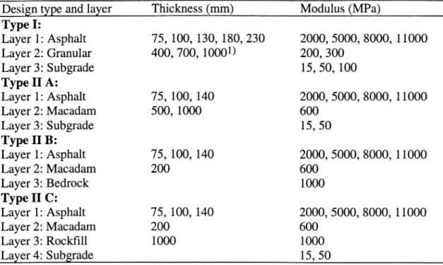
Pavements built according to the later Swedish Road Administration speci cations were simulated. Layer thicknesses and moduli for the calculated designs are shown in Table 1. Design type I is a conventional exible pavement. Type II includes a macadam layer (the surface being penetrated). A Poisson's ratio of 0.35 was used for all layers except a

stiff layer, which was placed at a depth of 3 m. Surface de ections, at different distances

from the load, and horizontal strain in the asphalt layer were calculated. The range of deflection under the load and asphalt strain are shown in Table 2. A CHEVRON program, modified by the Norwegian Institute of Technology [4] was used. The original program showed a drawback in that it occasionally gave unreasonable de ections close to the edge of the loading plate, even on fairly common pavements.

Table 1. Layer thicknesses and moduli of calculated pavements.

Design type and layer Thickness (mm) Modulus (MPa)

Type I: Layer 1: Asphalt 75, 100, 130, 180, 230 2000, 5000, 8000, 11000

Layer 2: Granular

400, 700, 10001)

200, 300

Layer 3: Subgrade 15, 50, 100 Type II A: Layer 1: Asphalt 75, 100, 140 2000, 5000, 8000, 11000 Layer 2: Macadam 500, 1000 600 Layer 3: Subgrade 15, 50 Type II B: Layer 1: Asphalt 75, 100, 140 2000, 5000, 8000, 11000 Layer 2: Macadam 200 600 Layer 3: Bedrock 1000 Type II C: Layer 1: Asphalt 75, 100, 140 2000, 5000, 8000, 11000 Layer 2: Macadam 200 600 Layer 3: Rock ll 1000 1000 Layer 4: Subgrade 15, 50

1) 1000 mm only on subgrade with moduli 15 and 50 MPa.

The reason for not including asphalt thicknesses thinner than 75 mm is to avoid most of the effect of decreasing strain with decreasing thickness, i.e. increasing deflections.

Table 2. Calculated de ection (DO) and asphalt strain (ea), average, min and max

values.

Design No. of D0 (mm)

8a (lim/m)

type calc. Average Min Max Average Min Max I 320 0.492 0.155 1.418 206 57 487 II 84 0.297 0.091 0.716 139 78 198

ESTIMATION OF ASPHALT STRAIN

Linear multiple regression was performed between the asphalt strain (Sa) (dependent

variable) and de ections at the distances of 0, 200, 300, 450, 600, 900 and 1200 mm

from the load centre (D0, D200, D300, D450, D600, D900, Dl200). The asphalt layer

thickness (Ta) and the type of pavement (I or H) were also tested as independent

variables. In regression analysis, the independent variables should preferably be independent of each other, but this is, of course, not true for the de ections. De ections decrease with radial distance from the load, and not at random, so strictly this is using regression analysis in a somewhat improper way. Nevertheless, the result is valid.

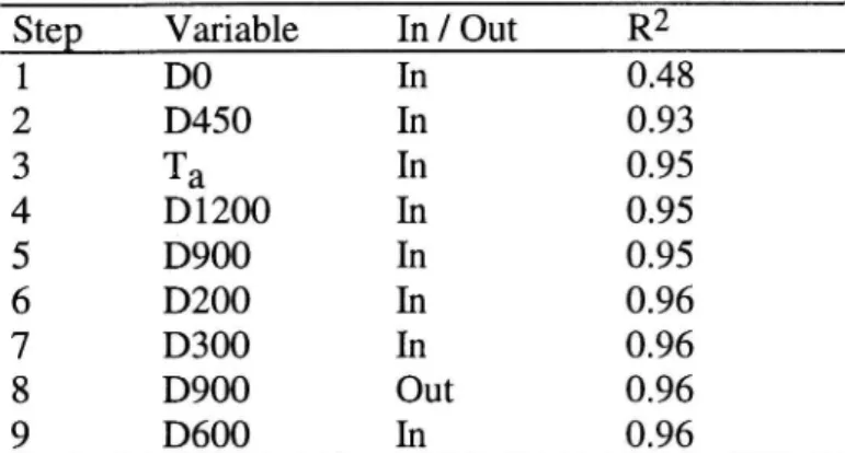
A stepwise regression yielded the result shown in Table 3. After only step two, the asphalt strain being a function of D0 and D450, a strong correlation coefficient (R2) is obtained. In step three, the asphalt layer thickness is added and the correlation coefficient is increased. In the following steps, de ections from different radial distances are added, but the increase in the correlation coef cient is low.

Table 3. Result of stepwise multiple regression, signi cant variables and correlation

coefficient (R2).

Step

Variable

In / Out

R2

1 D0 In 0.48 2 D450 In 0.93

3

Ta

In

0.95

4 D1200 In 0.95 5 D900 In 0.95 6 D200 In 0.96 7 D300 In 0.96 8 D900 Out 0.96 9 D600 In 0.96

One variable that does not give any significant contribution in explaining the asphalt strain is the type of pavement, which implies that there is no need to separate these when estimating the strain. Since the goal was to nd a simple way of presenting the results from FWD measurements, the asphalt layer thickness should preferably also be left out. This can be justi ed since the thicknesses are not known at every measuring point, and if the thicknesses are suf ciently known, the strain calculation can be performed with a

backcalculation procedure. A new stepwise regression analysis gave the relationship shown in Equation 1. The result is in microstrain if the de ections are given in mm. Ea: l7.8+2991.0*DO-9095.7*D200+9848.4*D300-6133.5*D600+2420.7*D900 (Eq. 1)

R2=0.96

The residuals, the differences between calculated and estimated (predicted) strains, are shown in Figure 1 (A). Historically, many measurements have been made with other sensor positions on the FWD. Typical positions have been 0, 300, 600 and 900 mm from the centre of load, or 0, 200, 450 and 900 mm. For these positions, the relationships are shown in Equations 2 and 3. The result is in microstrain if the de ections are given in mm.

a= 37.4+988.0*D0-553.0*D300-502.1*D600

(Eq. 2)

R2=0.93

8a= 36.3+1330.4*DO-1011.4*D200+21.2*D450-450.0*D900

(Eq. 3)

R2=0.94

Residuals are shown in Figure l (B and C). In Equation 2, D900 is not included, because

the contribution of this de ection in explaining the asphalt strain is small and the de ection is often low. In Equation 3, the contribution of D450 is small.

With one of the equations above, a specific de ection basin results in a speci c asphalt strain.

Asphalt strain calculated from de ections with the above equations is an estimate of the strain that will be calculated with the CHEVRON program after backcalculation of moduli. One exception to this is when the asphalt layer thickness is small, as earlier explained. From Figure 1, it can be seen that the deviation between calculated and estimated strain in most cases is lower than 10%, and seldom higher than 20%. If, however, the backcalculation is not performed well, or the used thicknesses are other than the actual thicknesses, the estimated strains may be more appropriate and closer to those that exist in the road.

In the introduction, it was said that earlier developed equations for weaker pavements should not be extrapolated for stronger pavements. To check the reverse, i.e. to determine whether Equation 1-3 could be used on weaker pavements, an example was calculated. The result is shown in Figure 2. This is the CHEVRON calculated strain compared to estimated strain, from CHEVRON calculated de ections. The simulated

road showed surface distress, and the high strains are theoretical. However, the

estimated strains are in reasonable agreement with the calculated strains, increasing with increased de ections and decreased asphalt layer thickness. This is essential if the estimated strain is to be used as a measure of structural condition.

Fi ure 1.

Predicted Value of Asphalt Strain [micro]

560

strain, in microstrain. A) Equation 1, B) Equation 2 and C) Equation 3.

Residuals, difference between calculated and estimated (predicted) asphalt

B)

C)

E:

m c o . -< n c o : n m c o . -< n m 3 ) I I I O) A IX ) O O C) _80. 100 100 80 60'

L

M

M

)

M

-S O O O O O O O \ 100 / + + \ 100 /

%&

+++ \ + + \\ _ N + ++ + | 200 200 / + i + \+ l 400 + 500 500 +.. 33 \+\ 300

Predlcted Value of Asphalt Stram [mlcro]

& + *; *: 3 w * + 300

Predlcted Value of Asphalt Stram [mlcro] ,/ "'10%

1600 T

1400 ' "' ' Calculated 1000 _" _ _ _ . - ' f(D0,D20,D45,D90) E1 <> f(D0,D20,D30,D60,D90) v 800 -E E 5 600 400 -200 " 0 l l l r l l l 40 60 75 100 130 180 230 280

Thickness of asphalt layer (mm)

Figure 2. Calculated asphalt strain (theoretical) and estimated strain from calculated de ections, using Equations 1-3.

Another test is to compare the estimated strains with those measured in Virttaa, Finland,

and reported in [5]. In this case, measured de ections are used in the equations. Measured, estimated and also BISAR calculated asphalt strains from two sections with different asphalt layer thickness are shown in Figure 3. The deviation between measured

and estimated (Equation 3) strains is on average 5% and at most 10%.

From the above examples, it can be seen that the estimated strain is somewhat dependent on which of the three equations is used. For that reason, it is recommended, that if possible, the same equation be used when comparisons are made.

350 T 0 O 300 80 mm asphalt % 5-3 . 250

e-%

V E] E 200 9 o' # I 2 150 Calc. BISAR % - D f D Est. Eq. 1 ft) 100 __ Llnequ & . E t E 2 equary 150 mm asphalt S' q. 50 -_ 0 Est. Eq. 3 0 i % ; l 1' l 0 50 100 150 200 250 300

Measured asphalt strain (um/m)

Figure 3. Measured, BISAR calculated and estimated, with Equations 1-3, asphalt

A STRUCTURAL INDEX

FWD measurements may be made for many reasons and often it is convenient to present the results in a way that is simple and does not require time-consuming calculations. These occasions may arise when there is a need to detect weak sections along a road, to divide the road into subsections with homogeneous structural condition, and possibly, as an extension, also to predict pavement performance, which may also lead to ranking maintenance and rehabilitation needs. Surface curvature index, radius of curvature and area are examples of expressions that are simple to use. An alternative is to use an expression based on the estimated asphalt strain. Such an expression, here named Structural Index (SI), might be:

SI = 1000 / Ea (Eq. 4)

Asphalt strain (Ea) in microstrain will give an SI value in the range of approximately 1 to 10. SI equal to 1 corresponds to a strain of 1000 and SI equal to 10 to a strain of 100 microstrain. The higher the value of SI, the better the structural condition and the stronger the pavement. A low value on a section of a road is an indication of a weak pavement or surface distress. It may also result when the road has a surface treatment or is unsurfaced. The strain may be estimated with the Equations 1-3. It may also be estimated/calculated in other ways, but this may of course affect the result and consequently also the structural index.

One advantage of talking of structural index instead of asphalt strain, is that at this stage it is not necessary to know whether the surface layer is sound or distressed.

Nevertheless, the structural index is a value that if desired can be used to predict

performance or residual life.

If a road, or network, is measured by FWD, the structural index can be used to divide

the road into homogenous subsections. A further step is to use the value, or actually the

estimated asphalt strain, together with an asphalt strain criterion, which also requires the traf c to be known. A rough estimate of remaining life can then be presented. The result can be used for ranking maintenance and rehabilitation needs. A ctitious example is shown in Figure 4. Once the decision to maintain or rehabilitate the road is taken, a more detailed analysis of the road, including FWD results, can be undertaken.

The structural index used as an independent variable in a performance model, cracking, is shown in Figure 5. The model was developed for low-volume urban roads, with surface layer of asphalt concrete, from a 5-year pavement performance study [6]. To describe a studied section, the median value of the SI was used, which proved signi cant in explaining many distresses. The horizontal lines in the figure, i.e. limits between different classes, are subjectively drawn to provide an example. The model can be used to predict future performance, provided that the SI is known.

Figure 4. Cr ac ki ng Figure 5.

j

Priority 1, remaining life approx. 0 year " Priority 2, remaining life approx. 1-3 years

Priority 3, remaining life approx. 4-6 years 555???- Priority 4, remaining life approx. 7-10 years

[2 Priority 5, remaining life approx. >10 years

Fictitious example of results from FWD measurements on a small road network, which also requires traf c data and asphalt strain criteria. Remaining life approximations are due to fatigue.

Age of asphalt layer (year)

Class 2 = "Over/ay

"

Class 3 = Unacceptable

- SI=1 Very weak pavement + Sl=2 "Normal" pavement

~ - Sl=3 Strong pavement

Performance model, cracking, for Swedish low volume urban roads, with surface layer of asphalt concrete. Average daily traf c less than 250, small number of heavy vehicles, freezing index 6700 C0*h and road width 6 m. The structural index wii 1 be affected by the same factors that affect the measured de ections, e.g. temperature. If temperature correction is necessary, the correction is simple to perform since there is only One value to correct. Correction factors may be developed from repeated FWD measurements on roads with ' typical asphalt layers (different types, thicknesses and age), preferably on days with large differences in temperature. Djärf has established Correction factors based on measurements (not published yet). For example, the SI is 20% higher at 10 OC compared to 20 OC, when measurements are made on a Swedish pavement with 130 mm of asphalt, and the centre

After overlay of a pavement, the SI will increase, as the de ections will decrease. The extent will depend on the SI before overlay and the thickness and stiffness of the overlay.

CONCLUSIONS

A simple structural index (SI) is presented. This is calculated solely from the de ections measured by FWD and based on the estimated horizontal strain at the bottom of the asphalt layer. The calculation is very simple and there is no need of supervision by an experienced engineer. Sometimes, this result from the FWD measurement is sufficient, at other times resources may instead be concentrated on a more detailed analysis. This

analysis does not necessarily include only the FWD data, since additional information,

such as local experience, distress data, field conditions (e.g. drainage), test pit results

and traffic data, is also important.

ACKNOWLEDGEMENTS

Most of this work has been sponsored by the Swedish Road Administration. The content of the paper re ects the View of the author.

REFERENCES

[1] Rohde G T, Smith R E and Scullion T, Pavement de ection analysis on sections where the subgrade vary in stiffness with depth, 7th International Conference on Asphalt Pavements, Nottingham 1992, Volume III pp. 280-295.

[2] Thompson M R and Hoffman M .S, Concepts for developing an NDT based asphalt concrete overlay thickness design procedure, Record No 945,

Transportation Research Board, 1983.

[3] Jansson H, Regressionssamband för beräkning av påkänning i asfalt ur

deflektioner mätta med fallvikt (in Swedish), VTI notat V 190 1992.

[4] Mork H, Analyse av lastresponsar for vegkonstruksjonar (in Norwegian), Doktor ingeniöravhandling 1990:6, Institutt for veg og jembanebyggning NTH,

Trondheim.

[5] Lenngren C A, Relating bearing capacity to pavement condition, Bulletin 1990: 1, Institutionen för vägteknik KTH, Stockholm.

[6] Jansson H, Modeller för tillståndsförändring på lågtrafikerade gator (ÄDT>250)