Voter Turnout and the Size of Government

(1)

Uppsala Center for Fiscal Studies

Department of Economics

Working Paper 2013:14

Voter Turnout and the Size of Government

(2)

Uppsala Center for Fiscal Studies

Working paper 2013:14

Department of Economics

November 2013

Uppsala University

P.O. Box 513

SE-751 20 Uppsala

Sweden

Fax: +46 18 471 14 78

V

oter

t

urnoutandthe

S

izeof

G

oVernment

L

inuz

a

GGeborn

Papers in the Working Paper Series are published on internet in PDF formats.

Download from http://ucfs.nek.uu.se/

(3)

Voter Turnout and the Size of Government

∗ Linuz Aggeborn†

November 4, 2013

Abstract

This paper investigates the causal link between voter turnout and policy outcomes related to the size of government. Tax rate and public expenditures are the focal policy outcomes in this study. To capture the causal mechanism, Swedish and Finnish municipal data are used and a constitutional change in Sweden in 1970 is applied as an in-strument for voter turnout in local elections. In 1970, Sweden moved from having separate election days for different levels of government, among other things, to a system with a single election day for political elections, thus reducing the cost associated with voting. This consti-tutional reform increased voter turnout in local elections in Sweden. The overall conclusion of this paper is that higher voter turnout yields higher municipal taxes and larger local public expenditures. Second, there is some evidence that higher turnout decreases the vote share for right-wing parties.

Key-words: Voter Turnout, Size of government, Sweden, Finland, Local public finance, Instrumental variable regression

JEL Classification Codes: D72 D70 H39

∗

I would like to thank Eva M¨ork and Mikael Elinder for many valuable comments. I would also like to thank Antti Moisio, Janne Tukiainen and the rest of the faculty at the Government Institute for Economic Research (VATT) in Helsinki where I collected the statistics for the Finnish municipalities. Furthermore I would like to express gratitude to Mattias ¨Ohman, Riikka Savolainen, Alex Solis, Erik W˚angmar, Agnese Sacchi and par-ticipants at the 2013 IIPF conference in Taormina (Sicily) as well as seminar parpar-ticipants at Uppsala University. An earlier version of this paper circulated under the title ”The consequences of voter turnout”

†

Department of Economics, Uppsala University. Uppsala Center for Fiscal Studies; Box 513, 751 20 Uppsala, Sweden. E-mail: linuz.aggeborn@nek.uu.se

(4)

1 Introduction

A number of democratic countries have experienced a fall in voter turnout rates since the end of the Second World War.1 Understanding the reason for this decline has been a major research question within the social sciences; voter turnout is considered by some to be important in order to sustain the legitimacy of the democratic process (Lijphart, 1997, p. 1-2). Certainly, there exist several normative arguments as to the importance of voter par-ticipation, as well as arguments reflecting a more skeptical stand regarding the value of high turnout rate.2 Nevertheless, voting is not only an isolated political action linked to the issue of democratic legitimacy but also, at least in theory, the basis for the formation of public policy. The purpose of this paper is to investigate the latter by taking a more positive approach that examines the causal effect of a variation in voter turnout on public policy. This paper is especially focused on policy outcomes related to the size of government, such as tax rates and public expenditures.

There is an ongoing discussion within the fields of political science and political economics over whether certain parties are favored when voter turnout declines.3 The focus in this case is whether a decline in voter turnout results in unequal representation. Regarding the actual effect on policy outcomes, there are two potential mechanisms through which turnout may affect policy. First, a drop in voter turnout may affect the policy po-sition of all parties running in an election as a result of an alteration of the median voter’s position. In accordance with the Hotelling-Downs model4, the median voter will be the decisive voter regardless of whether candidates are policy- or office-motivated, given certain assumptions. If voter turnout varies, policy outcomes may be different given a certain utility functions of the politicians.5 Second, a change in the voter turnout rate may result in a change in the vote share for the parties running in an election. The policy outcome may then change as a consequence of a party representation ef-fect.6 This would be more in line with the Citizen-Candidate model7, where political candidates implement their preferred policy if they win a political election.

1

Some countries such as the Scandinavian countries, Australia, Malta and Belgium seem to have a positive trend, but the overall picture shows a negative trend for established democracies for the time period 1945-1999. See (Franklin,2004, p.11)

2_See_Lijphart₍₁₉₉₇_{) and}_Caplan₍₂₀₀₈₎ 3

See for exampleLutz and Marsh(2007)

4_See_Downs₍₁₉₅₆₎ 5

Given that parties are office motivated they will react to a different position of the median voter since the median voter will be the decisive voter. This may also be true for policy-motivated candidates given that candidates may credibly commit to policy platforms and implements their suggested policy if elected. Voters are assumed to have singled peaked preferences.(Downs,1956, p. 28-31, 118). See alsoRoemer(1997) for a discussion.

6

SeePettersson-Lidbom(2008) andTyrefors Hinnerich(2008)

(5)

Empirically, the main challenge is to identify the causal effect of voter turnout on policy outcomes. For instance, a two-way causality is possible where voter turnout affects policy outcomes while a certain public policy may simultaneously influence whether people go to the polls. In this paper, I will use an institutional reform as an instrument for voter turnout in order to estimate the effect of turnout on policy outcomes. The empirical strategy involves using Swedish and Finnish municipal data and then exploiting the fact that Sweden changed its constitution in 1970 as an instrument for voter turnout.8 This constitutional change reduced the cost of voting in Swedish local elections and, according to economic theory, would result in an increase in the voter turnout rate. Finnish municipalities will act as a control group and I will argue that Finnish and Swedish municipalities are alike and act in similar constitutional settings. In Finland however, local elections and national elections are held on separate days at two year intervals, similar to the system in Sweden before 1970.

By investigating the causal link between voter turnout and the size of government, we may gain insight into the policy implications from the ob-served decline in voter turnout that many democratic countries have expe-rienced. Does a variation in turnout actually change policy outcomes? In this paper, I find support for this theoretical cogitation. More specifically, the constitutional change in Sweden in 1970 did increase voter turnout. The increase in turnout also resulted in higher municipal taxes and larger local public expenditures. In addition, there seems to be some evidence that po-litical parties belonging to the right-wing block were disfavored when voter turnout was increased.

2 Related litterature

In the field of political economics, the causal link between voter turnout and policy outcomes has generally been investigated using cross-country approaches. These results are interesting, but the question remains as to whether the causal link has been identified. Other papers have addressed the matter by studying the extension of the franchise. My paper contributes by combining features that together constitute a better setting for capturing the causal mechanism. First of all, I make use of an institutional change to get exogenous variation in turnout, which enables me to estimate the causal effect of turnout on policy outcomes more convincingly in a second stage. Second, municipal data from Finland and Sweden are very suitable due to the high degree of similarity between the Finnish and the Swedish political

8

Regarding voter turnout rate with and without a common election day,Oscarsson et al. (2001) has investigated the matter by studying Sweden and other comparative countries and concludes that a common election day seems to be one factor the government may use if they want to increase voter turnout.

(6)

systems. As for the matter of external validity, it seems reasonable that the result may the generalizable given that tax rate and public expenditures are universal outcome variables.9 Lastly, the first stage analysis of whether a change in the cost associated with voting will influence voter turnout is interesting in itself as it addresses the public choice question whether the cost associated with voting will affect the choice to participate.

Let us begin by reviewing those papers that have an emphasis on the extension of the right to vote. Lott and Kenny(1999) focus on the extension of the voting franchise in the U.S. during the 19th and 20th centuries. More specifically, they investigate the women’s right to vote and find that the extension of the franchise resulted in more liberal policies and an increase in public spending. According to Lott and Kenny(1999), there is a gender gap between the way that men and women vote, one potential explanation being that women are more risk-averse than men. According to the authors, women’s fears of being left alone as sole breadwinners with the responsibility of raising children creates a higher demand for higher public spending (Lott and Kenny,1999, p.1188).

Husted and Kenny (1997) focus on the abolition of literacy test and poll taxes in certain U.S. states during the 20th century. According to

Husted and Kenny (1997) The U.S. Voting Rights Acts of the 1960s and 1970s resulted in an increased turnout rate, especially among poor groups in the American society. This extension of the voting franchise resulted in larger redistribution and greater welfare spending. (Husted and Kenny,

1997, p.79).

The results from the two papers above indicate that policy outcomes will change when the electorate encompasses a larger share of the adult inhabitants. Other papers have instead focused on countries that had a full extension of the franchise, but where the voter turnout rates vary. An increase in voter turnout may be interpreted as a de facto enlargement of the voting collective which may yield a similar effect on public policy as an extension of the franchise. Additionally, the actual extension of the voting franchise may in turn be endogenous in itself, which was the conclusion of

Acemoglu and Robinson(2000).

Mueller and Stratmann (2003) use a cross-country approach to investi-gate whether lower turnout will have an effect on economic growth, income inequality and public sector growth. They conclude that a higher voter turnout rate is associated with a larger public sector. Furthermore, they find support for what the authors denote as a class bias where lower turnout rate leads to more unequal income distribution. Among other methods, they use an instrumental variable approach in order to address the probable en-dogeneity of voter turnout. Mueller and Murrell (1986) also apply

cross-9

The question remains as to whether the results may be generalized to countries where the voter turnout rate is initially lower than in Finland and Sweden.

(7)

country analysis. Their focus is mainly on the link between interest groups and the size of government; however, they also find that the turnout rate and population will have a positive impact on the magnitude of the public sector. The idea of class bias is also investigated inHill and Leighley(1992) who use data from American states. They conclude that the underrepresen-tation of the poor will result in class bias. For example, they conclude that welfare spending is lower in states where voter turnout among the poor is low.

Fumagalli and Narciso (2011) use the same data set as Persson and Tabellini(2005) in their cross-country study but argue that the voter turnout rate is the transitional variable between the constitution and the economic outcome. Persson (2003) does not study voter turnout but rather the eco-nomic effects of constitutions by applying a cross country approach and finds, for instance, that a majoritarian voting system is associated with narrower spending focused on certain groups of marginal voters whereas a propor-tional voting system is associated with broader spending directed towards all groups in a society. All of these studies rely on cross-country analysis and the causal interpretation of these results may be questioned. The problem with a cross-country method is that countries are diverse by nature and it is difficult to control for all differences between them. Most likely you will have omitted variables resulting in biased estimates.

Let us now switch our focus to studies using more disaggregated data.

Fujiwara(2010) examines a voting reform in Brazil entailing the introduction of electronic voting. The reform resulted in a 10 percentage increase in the share of valid votes cast. Voting is mandatory in Brazil, therefore the reform did not increase the turnout rate; instead it augmented the share of valid votes from people that were illiterate. The result was that left-wing parties increased their vote share and that policy outcomes changed, for example public expenditures on healthcare increased. (Fujiwara,2010, p. 38-39)

Fowler (2013) employs Australian data and focuses on the implementa-tion of mandatory voting. When voting became mandatory, working-class citizen increased their share in the electorate resulting in more votes for the Labor Party. Furthermore, the implementation of mandatory voting laws increased pension spending in Australia in comparison to other OECD countries. (Fowler,2013, p. 159-160)

Horiuchi and Saito (2009) on the other hand apply Japanese munici-pal data and election day rainfall as an instrument for turnout to address the problem with potential endogeneity of voter turnout. They find that a higher voter turnout rate in a municipality results in higher intergovern-mental transfers to that municipality. The authors discuss pre- and post election political incentives and hypothesizes that projects financed by the central government are targeted at those legal entities with a higher political participation rate. The authors propose that elected governments act in this manner to maximize the probability of reelection. See alsoMartin(2003).

(8)

Lastly, variation in voter turnout may also influence the vote share for different political parties and thus indirectly the policy outcome. The above mentioned papers put the voters’ preferences in the center. Other papers, however, emphasizes the politicians, as in studies that focus on the effect of party representation on policy. By applying a regression discontinuity approach to Swedish municipal data,Pettersson-Lidbom (2008) shows that party representation on the municipal level affects both policy and economic outcomes. This conclusion is interesting and points towards the conclusion of the Citizen-Candidate model where the preferences of the parties will determine policy outcome. Lee et al. (2004) also find evidence in favor of the Citizen-Candidate model in which elected politicians implement their preferred policy. Elections to the U.S. House of Representatives between two candidates from opposing parties with equal local support do not seem to moderate the pursued policy of the elected representative in comparison to candidates elected in a Democratic or Republican-majority district. (Lee et al.,2004, p. 807)

Tyrefors Hinnerich(2008) applies an RD estimation procedure to Swedish municipal data from 1959-1966 to study the partisan effect on policy out-come. According to Tyrefors Hinnerich (2008) and in line with Pettersson-Lidbom (2008), parties do matter for policy outcomes; interestingly, how-ever, there seems to be a convergence in policy in those municipalities where the right-wing block and the left-wing block are more equally sized ( Tyre-fors Hinnerich,2008, p.8).10

The remainder of my paper is organized as follows: The following section presents a theory for voter participation on the individual level. Later in the same section I will present a simple model of voters’ preferences regarding the size of government. Next, the econometric strategy is presented in the identification strategy section followed by a description of the Finnish and Swedish local political system and a description of the data used in the paper. The results are then presented, followed by robustness analysis and a conclusion. Further regression tables may be found in Appendix 3.

3 Theoretical framework

The focus of this paper is the causal link between voter turnout and policy outcomes and we therefore need a theoretical foundation both for the in-dividual choice regarding voting and a model of preferences for the size of government.

In this paper I use a choice model related to the model presented by Fio-rina (1976) and described in Mueller (2003) which suggests that we should

10_{This conclusion lies somewhere in-between the Citizen-Candidate model and the more}

classic Hotelling-Downs model where only voter preferences will matter for policy out-come.

(9)

view the individual’s choice to vote in light of the expressive voter hypothe-sis. This model is an extension of the classic Public Choice model of voter participation.11 Voters in this model obtain utility not only from having a particular political outcome realized, but also from expressing their opin-ions in an election together with having a degree of civic duty. The model consists of the following simple equations

P (vote) = P B + D − C (1)

D = D0+ B (2)

P denotes the probability of being the decisive voter in an election, C the cost associated with voting and B the benefit (gain in utility) of having one’s preferred policy alternative implemented rather than some other. In this model, D is consists of two different variables, namely B which is the benefit of having a certain policy expressed and D0 is the ”civic duty part”12 of the D-expression. B is in this model important in itself and not just as a part of the P B in the first equation, meaning that voters both get utility from having a specific policy implemented together with a positive utility associated with expressing their opinion regarding this specific policy. (Mueller,2003, p. 320). 13 _{The cost of voting should be understood as the}

alternative cost of voting – for example lost income during the time you are at the polling station. One may also think of the cost of voting as the cost of acquiring information regarding the election and the choice of political party.

D0 might also be interpreted to mean that voting is also an act of social norms and not only an outcome of an individual utility optimization based on the cost and benefit of voting (Mueller,2003, p. 320). Therefore it might be utility maximizing to vote given that one’s utility function incorporates a social norm variable, such as D0. All individual parameters are however influential in the individual voting decision; a decrease in the cost of voting, C, will ceteris paribus increase the turnout rate.

Let us further assume that there is some relationship between the civic duty portion of the individual voting choice model, D0 and the degree of

11

The problem with the classic model is above all that it predicts that, given that voters are rational, the turnout rate should be 0.

12

SeeGerber et al.(2008) for an empirical investigation of the relationship between civic duty, social norms and voter turnout.

13

Note that D is here more explicitly specified than the more residual explanation given inRiker and Ordeshook(1968) where D is just a taste for voting.

(10)

education14, such that D0 = f (Ei).15If more highly educated groups have a

higher level of D0, then they will be overrepresented among the voters when the voter turnout rate is less than 100 percent.16 This implies that there is a difference between the participating and the abstaining voters. The hypothesis is that less educated groups abstain from voting because their net utility gain is negative in the individual voting choice model.17 If some of the other variables in the individual voting choice model are altered, it should affect the voter turnout rate. For example, if the cost associated with voting decreases, voter turnout rate should increase everything else being equal. The share of highly educated voters VH will then be lower than

before because this would result in an inflow of less educated voters VL. 18

↓ C → ↑ VL VH + VL

(3) Let us now turn to the issue of demand for public goods to examine the implications from the arguments above. The assumed utility function for voters and the constraint regarding the provision for public goods are presented below.19

14_{This argument below also holds if we assume a direct relationship between personal}

income and level of civic duty.

15

See Appendix 1. Here I assume a linear relationship between education and civic duty. One may argue that very highly educated voters at some point experience a decrease in their civic duty because they realize that they have a better knowledge of the society than the people involved in political life. This effect is however not straightforward.

16

I assume here that B in the D expression is equal between high educated and low educated.

17

The argument above regarding the link between higher education and a higher prob-ability of voting is in itself an empirical question. There are a number of papers in the empirical literature in which the authors argue that higher education increases the probability of voting. See for exampleSigelman et al.(1985). Some more recent papers have not found this link between education and voter participation. Knack and White (2000) study voter registration, but find that the possibility of election day- registration does not result in a lowe bias regarding the prevalence of highly educated groups in the potential electorate. Solis(2012) argues that the long-accepted positive relationship between education and turnout is a spurious correlation. In this paper, the focus is not on this intermediate step, but rather on the effect of a variation in turnout on policy.

18

This may be compared to the Meltzer and Richard(1981) model in which the median voter will be the decisive voter in a country with a democratic voting rule. According to this model, the decisive voter will be equal to the person with the median income which is in turn equal to the person with the median productivity in a society.

19

The model is based on the simple model of public finance presented by (Persson and Tabellini,2002, p.48-49)

(11)

3.1 Voters’ utility schemes Ui= ci+ q(G) (4) ci= (1 − t)wi (5) t ∈ [0, 1] (6) W = ∞ X i=0 wi (7) G = tW (8)

Voters are assumed to have two sources of utility. First, they get utility from private goods consumption, ci. Second, they get utility from the

provi-sion of public goods according to some concave function q(G). Hence, voters’ utility function is quasilinear. To consume private goods, voters require an income and the level of private good consumption is therefore a function of the individual wage wi. The government taxes voters in order to finance

public goods consumption, which is G, and the tax rate is proportional.20 The government must balance its budget and the total amount of public good provision must therefore be equal to the total wage level in the society multiplied by the tax rate. Public goods spending may not be focused on a specific group, i.e., it is a pure public good. Second, the government taxes all individuals with the same tax rate, t (Persson and Tabellini,2002, p.48-49). The utility function for the voter may then be rewritten as:

Ui = (1 − t)wi+ q(G) (9)

Ui = wi−

Gwi

W + q(G) (10)

Below I define some properties of the utility function. The first order condition of the utility function with respect to G is

∂Ui ∂G = − wi W + q 0 (G) = 0 (11) Gi= q−1G ( wi W) ≡ G( wi W) (12)

If the individual wage level as a share of the total wage level, wi W, will

increase, then the marginal utility from public goods provision will decrease. In conclusion, the demanded level of public goods will depend on the wage vis `a vis the mean wage level in society. Public goods provision therefore has a redistributional aspect following from the fact that voters have a quasi-linear utility function. If you already have a relatively high private good consumption as a result of a higher relative wage level, your demand for

(12)

public goods provision will decrease. This is because individuals are net contributors to the financing of public goods (Persson and Tabellini,2002, p.48-49).

If parties react to incentives in accordance with the Hotelling-Downs model, they will reposition themselves in accordance with the position of the median voter.21 Given the argument that voters with a higher personal income level (a longer education) have a higher probability of voting and that parties may commit to policy platforms, a lower voter turnout rate is associated with lower taxes and lower public expenditures. 22

The Citizen-Candidate model on the other hand predicts that politi-cal candidates implement their preferred policy if elected. A lower voter turnout rate would in this case alter the vote share for certain political par-ties. Instead of altering the position of political parties, votes are driven towards those parties whose policy platform consists of more redistribution and therefore higher taxes when turnout is increased. It is uncontroversial to assume that this equal left-wing parties. The bottom line is that voter turnout will have an influence on policy regardless of whether we believe in the Hotelling-Downs model or the Citizen-Candidate model. The purpose of this paper is not to evaluate which of these model that has the best pre-dictions, but rather to investigate the link between voter turnout and policy outcomes which is related to both of these models. My suggestion as to how this might be accomplished is presented in the next section.

4 Identification strategy

We are likely to have a problem with two-way causality between voter turnout and policy outcomes. Given the purpose of this paper and the discussion in the theoretical section, the ideal experiment would be to ran-domize cost of voting in many legal entities within the same country and then estimate the causal effect of a variation in turnout on policy outcome.23

Because this is not possible, one solution would be to use an instrument for exogenous variation of the cost for voting and then estimate the effect of turnout on policy outcomes in the second stage. In order to apply this em-pirical strategy, a suitable control group similar to the treatment group is

21

This is under the assumption of single peaked preferences among the voters. Convergence towards the median voter’s position may also be the case, given certain assumptions, if parties are policy motivated instead of office motivated. SeeWittman(1973),Wittman (1976),Duggan and Fey(2005) andRoemer(1997).

22

In reality, the actual voter turnout rate is not known to the running parties before the election. Policy platforms, however, are announced before the election. I assume here that parties base their policy platforms on an approximation of the expected voter turnout rate which is grounded on the information of voter turnout rates in previous elections.

23

This is in line with the theoretical model where the cost of voting is related to voter turnout.

(13)

needed.

In this paper, Finnish and Swedish municipal data will be used. Sweden changed its constitution in 1970 resulting in a number of new features in the Swedish election system. The constitutional reform affected both the central government and the local government and throughout this paper I will consider this change in the Swedish constitution in 1970 as a reform package and use this as an instrument for turnout.

To begin with, a common election day for parliamentary, county and municipal elections was introduced and the previous four year mandate pe-riod was replaced by a new three year mandate pepe-riod (Oscarsson et al.,

2001, p.31). Before the reform, Sweden held elections every second year, with county and municipal elections held together in one year and a parlia-mentary election held separately two years later. The mandate period was four years for all three levels of government.

Additionally, the bicameral parliamentary system was abolished and Sweden introduced a unicameral parliamentary system. Before 1970, di-rect elections were held for the second chamber and indidi-rect elections to the first chamber through the county councils (Oscarsson et al.,2001, p. 21, 25, 28-29).

Parallel to the constitutional change regarding the election system, a municipal merger reform took place. In 1966, Sweden had approximately 900 municipalities and in 1974, after the merger reform was completed, 278 municipalities remained. The foremost reason for reducing the number of municipalities was the fact that many municipalities were very small in terms of population. Higher demands on municipal ability to provide a variety of services and a need for each municipality to be functionally independent and able to manage itself within the municipal borders were also important arguments for the municipal merger reform. (Erlingsson et al.,2010, p.15)

The constitutional change that took place in 1970 may be characterized as parts of the individual voting choice model. The introduction of a com-mon election day led to a lowering of the costs associated with voting in local elections. According to the theoretical model, a lower cost associated with voting should increase turnout. At the same time, the municipal merger reform resulted in larger municipalities so that the chance of being the de-cisive voter in an election was reduced after the merging of municipalities which should then have led to a lower voter turnout in turnout. However, the chance of being the decisive voter even before the merger reform was extremely small. Likewise, the introduction of a unicameral parliamentary system should increase voter turnout because it enhances the importance of voting in a parliamentary election.24 The effect of the introduction of a three year mandate period is more difficult to categorize as a positive or negative

24

The parliament has now one legislative body that is directly elected by the people. Prior to 1970, only one of two chambers of parliament was directly elected.

(14)

factor for voter turnout. One may think that it is less important to vote because the voters get a new chance every three years. However, the voters may suspect that reforms are implemented faster with a shorter mandate period and that it is therefore more important to vote. The different reforms and their expected effects on turnout are summarized in the table below. I discuss the identifying assumption of the first stage IV-analysis with regard to these expected signs in section5.1

Reforms Expected sign Common election day ++ 3 year mandate period +/-Unicameral parliamentary system +

Municipal merger

-This paper will use instrumental variable regression to estimate the causal effect of voter turnout on policy outcomes. OLS estimates would most likely be inconsistent as a result of two way causality between turnout and policy. The first stage in the IV-analysis consists of a difference-in-difference regression with a binary treatment variable for the Swedish municipalities and a treatment period from 1971. The control group is the Finnish mu-nicipalities. In the second stage analysis, I will regress the instrumented turnout variable on policy outcomes. Both Sweden and Finland apply the same election schedule whereby elections are held in the fall of each election year and the newly-elected councils meet in the beginning of the following year.25 The regression equations are thus expressed as:

Yi,t = β0+ β1T urnouti,t+ β2Wi,t+ τt+ fi+ ui,t (13)

T urnouti,t = πi,t+ π1Zi,t+ π2Wi,t+ τt+ fi+ ui,t (14)

Yi denotes the dependent variable of interest. In total, I will have three

de-pendent variables: the municipal tax rate26, total public expenditures27and vote share for the right-wing bloc.28 β0 is the intercept. β1 is the parameter

of interest which estimates the effect of a variation in turnout on the depen-dent variable. The fixed effects are denoted as τt and fi respectively. ui,t is

the error term.

25_{This will be important in my case because municipal mergers took place 1969-1974 in}

Sweden. In the local election of 1970, for example, people voted for the municipal coun-cils that were legally in place in January 1971, at which time there were approximately 100 fewer than the total number of active municipalities in 1970. Therefore, data re-garding turnout in the 1970 election will be merged with municipal finance statistics for the year 1971 and so on. This is done for the entire data panel. Election result may only have an effect on policy after the new councils are in session.

26_{Denoted utdebitering per skattekrona in the Swedish printed statistics and skatte¨}_orets

v¨arde in the Finnish statistics.

27_{Denoted summa utgifter. in the Finnish printed statistics 1967-1972 and egentliga}

ut-gifter between 1972 and 1977 and utut-gifter total in the Swedish printed statistics.

(15)

Equation (13) thus denotes the second stage in the IV-model. Wi,t is

a vector of control variables. Both time and municipal fixed effects will be applied in the regression analysis to control for unobservable factors that are constant between entities or over time. In the first stage equation (14), we have a difference-in-difference setup. Variable Zi,t takes the value 1 if the

observation belongs to the treatment group (Swedish municipalities) and the treatment period (any year after 1970).

The municipal mergers that took place in Sweden between 1969 and 1974 are of particular concern because these mergers are most likely related to policy outcome. Tyrefors Hinnerich (2009) studies this merger reform in Sweden and finds evidence that municipalities that were going to merge would free-ride and accumulate fiscal debt the years before the afore men-tioned merger. Jordahl and Liang(2010) focus on the earlier merger reform in Sweden in the 1950’s and find that municipalities that were going to merge accumulated new debt for four years prior to the merger. I will ad-dress these merger effects in a number of ways. First, Swedish municipalities affected by the merger received a so-called transitional grant to avoid sudden change in the municipal tax rate. These transitional grants are included in the total state grants variable for the Swedish municipalities. The vector of covariates includes a number of interaction variables, in order to control for potential merger effects in the Swedish subsample.29 The values have been deflated and are expressed in USD for relevant variables.30 The covariates used in the analysis are population, state grants31_{and tax base}32_{, together}

with merging dummies and dummies for newly created municipalities as well as interaction terms.

Voter turnout is assumed to be constant during a mandate period in the baseline specification, meaning that the turnout rate in a municipality will take the same value for the years up until the next election. This may be problematic due to the increase in the number of included observations where there is no any actual variation in the data. Policy outcomes may however be affected by the turnout rate with a lag and municipal councils may, for example, change the tax rate several times during a mandate period. The

29

To start with, I will create dummy variables taking the value 1 if a municipality was merged with another municipality in a given year. Second, I will create a dummy variable indicating whether the observation belongs to a municipality that was newly created in a given year. These dummy variables will be interacted with tax base and population in order to control for the effects of a sudden increase in the number of inhabitants and the tax base due to merger.

30_{First, I express the nominal values in USD. Then I use a price index based on CPI, with}

2005 as base year, in order to deflate the nominal values into real values.

31

Denoted as skatteutj¨amningsbidrag in the Swedish statistics and statsbidrag och ers¨ at-tning and summa inkomster av staten in the Finnish statistics that are divided into rural municipalities and towns.

32_{Antal skattekronor in the Swedish statistics and Antal skatte¨}_{oren in the Finnish}

statis-tics. In my judgment, these are the best corresponding variables for tax base in the Finnish and the Swedish data.

(16)

treatment of turnout may therefore have several effects during a mandate period. However, in the robustness section the years in which no election took place will be dropped and the econometric analysis redone. This will be performed with means for all included variables within a mandate period and a mean only for the dependent variable, but where all independent variables are expressed in their yearly values. 33

4.1 Standard errors

Another econometric obstacle is the estimation of the standard errors. Swedish and Finnish municipal data are probably correlated within groups where each municipality cannot be considered a random observation independent of other observations. This concern was first addressed by Moulton (1986) who concludes that that if there is some within-group correlation the esti-mated standard errors will be down-ward biased as a result of a correlation in the error terms. This is often denoted as the Moulton-problem and may result in false statistical significance of point estimates.

One solution is to cluster the standard errors on some appropriate level. One may think that the country level would be appropriate because all municipalities in Sweden and Finland will be correlated to some degree in addition to the fact that the treatment used as instrument was implemented on the national level. The problem then is that I would only have two clusters which are not enough for correct asymptotic properties.

I chose two different strategies in order to address the concerns regard-ing the estimation of the standard errors. In both Finland and Sweden, municipalities are grouped together in counties34. The counties constituted the central government on the regional level. In Sweden, direct political elections are held for the county councils35_{, but there are no such elections}

in Finland. The government appointed a representative, a landsh¨ovding, in each county, in both Finland and Sweden. Some of the responsibilities of the Swedish landsting, such as hospitals, are placed on the municipal level in Finland.

In the Swedish subsample, it is possible that there are clusters of turnout at the county level for various reasons. For example, regional policy may induce whether one casts a vote for the county councils. Because municipal elections are conducted at the same time, this may also affect voter turnout at the local level. However, there are other possible correlation effects that may be present in both the Finnish and Swedish subsample because the counties are responsible for implementing government policy on the local

33_{This strategy was chosen due to my inability to control for merging effects if taking}

means for all included variables because some municipalities did merge during a mandate period.

34

L¨an in Swedish.

(17)

level. Furthermore, the counties in both Finland and Sweden were created in the 17th century and may in some sense be considered as legal entities for a regional structure of socio-economic characteristics that may have an effect on voter turnout. The instrument in this paper is the constitutional change in Sweden in 1970. It is possible that the treatment effect is clustered on the county level as a result of similar political history within a county. Altogether, this may have an impact on voter turnout.

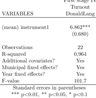
In all, clustering at the county level leads to 34 clusters. One may argue that this is too few.36 Additionally, the constitutional change in Sweden in 1970 was a national reform and I therefore only have one treatment group and one control group, however 10 years in total in my panel. To further address the standard errors issue, I will also estimate standard errors using the approach suggested in Donald and Lang (2007). Briefly, this is a two-step procedure by which data is aggregated for each different group and time combination37, thus reducing the number of observations by collapsing the data. This Donald and Lang specification will be used for the first stage IV and the reduced form specifications, which are the estimations where the binary instrument is directly applied. Formally:

Yi,t = β0+β1Wi,t+γ2Swedeni∗yeart+γ3F inlandi∗yeart+τt+fi+ui,t (15)

ˆ

γi,t = β0+ β1Xi,t+ β2Swedeni+ β3F inlandi+ β4yeart+ ui,t (16)

ˆ

γi,tconstitutes the predicted values from the first step (covariate adjusted

groupe means) in the Donald and Lang procedure. I use the number of observation in each group and year as weights and estimate equation (16) by weighted least squares (WLS). Wi,t is the same vector of covariates used

in other specifications in the paper. β1is the parameter of interest and Xi,tis

the binary instrument taking the value 1 if the observation belongs to Sweden and any year after 1970. τt and fi are municipal and year fixed effects.

In equation (15), yeart and Swedeni and F inlandi country dummies are

interacted with each other resulting in one binary variable for each time and group combination. By collapsing the data, we end up with two observations from each year – one for the Swedish subsample and one for the Finnish. In the second step (16) I use the saved predicted values to run a regression where I include the variable of interest together with dummy variables for Sweden and Finland and dummy variables for each of the years in my panel. In sum, both these methods yield more conservative standard errors than ordinary robust standard errors which only compensate for heteroskedastic-ity in the residuals. Let us now turn to a description of the Swedish and Finnish institutional settings and a discussion of the identifying assumptions.

36

In a humorous reference to Douglas Adam’s novel The Hitchhiker’s Guide to the Galaxy

Angrist and Pischke (2008) suggest that you should at least have 42 clusters. The

number of clusters needed remains under debate.

(18)

5 Institutional setting - Sweden and Finland

This paper is based on a similar identification strategy to that inDahlberg and M¨ork (2011). Sweden and Finland have a long common history, and their political institutions display a high degree of similarity. 38 _{The focus in}

this paper is on local governance and I will argue that Swedish and Finnish municipalities constitute a suitable testing ground for empirical work in pub-lic and political economics due to the fact that they are highly independent and exist in two similar institutional environments.

Swedish and Finnish municipalities have the right to collect taxes and they are free to choose their own tax rate. The municipal tax in one of the primary income sources for the municipalities and they may borrow money on the financial market. They receive grants from the central government and provide public services such as social assistance, elderly care and child care and as a result they are fundamental welfare suppliers in each country. Between 1967-1977, both Finland and Sweden were divided into counties, or län, in which the so called länsstyrelse was the central governments represen-tative in each county. In Sweden, there is also a regional political structure within the same borders as the counties called landsting. Political elections are held to the landstingsfullmäktige whose prime responsibility is health care. In Finland, health care is the responsibility of the municipalities, but smaller municipalities tend to cooperate over health care.

Both Finland and Sweden are sparsely populated where the inhabitant are clustered in a number of larger cities. The northern parts of each country are even more sparely populated than the southern parts. As you can see in the graphs displayed in the robustness analysis section, a few municipalities have much higher public spending that the majority of the municipalities.

Direct political elections are conducted to fill municipal council seats every fourth year (in Finland and in Sweden before 1970) and each third year (in Sweden after 1970). Both countries conduct elections through a PR voting system.39

My first stage uses a difference-in-difference approach and the main iden-tifying assumption behind DiD estimation is that of parallel trends in the variable of interest. Swedish municipalities should have a parallel trend in turnout in comparison to the Finnish municipalities and the development in turnout rate should look the same if the Swedish municipalities had not experienced the constitutional change in 1970. I will present a graph be-low illustrating the average turnout rate in local elections for Swedish and Finnish municipalities. As you can see, the average voter turnout rate is higher in Sweden for the entire time period, but there is an increase in 1970 for the Swedish subsample. After 1970, the trend in each country is also

sim-38_{Finland was a part of Sweden from the early middle ages up until 1808.} 39

SeePettersson-Lidbom(2012) and (Dahlberg and M¨ork,2011, p.482-484) for a descrip-tion of Swedish and Finnish local governments.

(19)

ilar, but the difference in turnout rate is larger. Note that voter turnout is displayed as constant during a mandate period in this graph. The conclusion is that Finland and Sweden have a similar trend in this variable.

60 70 80 90 Voter turnout in % 1960 1970 1980 1990 2000 year

Turnout Sweden Turnout Finland

Data source: Statistiska Centralbyrån (2013b) and Statistikcentralen (2013c). My own assembly

Voter turnout local elections aggregated data

One important assumption in this paper is that Finland and Sweden are similar countries. In addition to the description of the responsibility of the local sector above, I show some figures below displaying voter turnout in parliamentary elections, GDP per capita, the central government’s taxation in percentage of GDP and local taxes as percentage GDP. For some of these variables I only have access to data for a shorter time period.

0 10000 20000 30000 40000 GDP/capita 1970 1980 1990 2000 2010 year

GDP/capita Sweden GDP/capita Finland

Data source: OECD.stat (2013d)

GDP per capita USD − current prices − current PPP’s

70.00 75.00 80.00 85.00 90.00 95.00 Turnout in % 1940 1960 1980 2000 2020 year

Turnout Sweden Turnout Finland

Data source: Statistiska Centralbyrån (2013a) and Statistikcentralen (2013a)

Voter turnout in parliamentary elections

0 10 20 30 40 50

Central government taxes in % of GDP

1972 1973 1974 1975 1976 1977 1978 1979 1980 1981 1982 1983 1984 1985 year

Sweden Finland

Data source: OECD.stat (2013a)

Central government’s taxes as share of GDP

0 10 20 30 Local taxes in % of GDP 1972 1973 1974 1975 1976 1977 1978 1979 1980 1981 1982 1983 1984 1985 year Sweden Finland

Data source: OECD.stat (2013a)

(20)

5.1 Threats to identification

Regarding instrumental variable regression, we need instrument exogeneity. Is there reason to believe that the instrument should affect policy outcomes directly and not through the turnout variable? The 1970 constitutional reform in Sweden was decided by the central government and the policy variables in focus in this study are in the legal jurisdiction of the municipali-ties. If an effect is present between the constitutional change and the policy outcomes on the municipal level, then it must be an indirect effect.

In the years prior to the constitutional reform, a public constitutional inquiry had taken place. When this inquiry was presented, none of the political parties in the Swedish parliament were in favor of the idea of a common election day. The choice of a common election day was instead the result of a compromise as it was considered vital that all political parties unanimously agreed on the constitutional change. In fact, it was the issue of the single chamber parliamentary system that divided the political par-ties. The Social Democrats wanted to keep the bi-cameral system and the right-wing parties supported a unicameral parliament. The upper chamber had a local connection since its members were elected indirectly through the county councils and the Social Democrats argued that the local connection in national politics would be lost if the upper house was abolished. The center-right parties, however, ultimately prevailed against the two-chamber parliamentary system. As a compromise, a common election day was in-troduced and the two-house parliament was replaced by a single chamber parliament. Because all elections were grouped together, there was still some local connection in the national election in accordance with the compromise. (Oscarsson et al.,2001, p.29-31).

Historical records show that the outcome of the constitutional change in Sweden was largely due to political logrolling on the national level. The municipalities were undeniably affected by these reforms, but it is difficult to imagine why they should affect policies such as tax rates and public spending directly because many of the decisions were made over the heads of local politicians. Swedish municipalities have a high degree of independence and they may set public policy without consulting with the central government. Regarding the new, and shorter, 3 year mandate period that was introduced at the same time, it is, in some sense, easier to argue that this reform could affect the municipal policy outcome. There is however no clear-cut theoretical prediction as to what we should expect from such a reform.

In conclusion, there is no particular indication that the constitutional re-form should have affected the policy outcomes in the Swedish municipalities and as a consequence, no obvious reason to believe that we have a threat against the assumption of instrument exogeneity.

Another threat against identification is that the monotonicity assump-tion of the first stage is not fulfilled. Formally, we need w1− w0 ≥ 0∀i,

(21)

where w is the binary indicator for the DiD instrument in the first stage. In essence, implementing the constitutional reform in Sweden cannot decrease voter turnout in some municipalities. To examine this, I will rerun my first stage analysis for different subsamples: One group with municipalities that were merged and one group with municipalities that were not merged, and two other regression specifications where highly populated and less popu-lated municipalities are analyzed separately. The results will be presented in the robustness analysis section.

6 Data

The data were collected from Statistics Sweden and Statistics Finland, from the publication series ˚Arsbok för Sveriges kommuner, Kommunal Finansstatis-tik, ˚Arsbok för Finland, Statistisk Rapport, Allmänna valen and Kommunal-valen.40 Some of the data have been downloaded in digital format; however the data are not available in digital form for the majority of the years covered and the variables used. Data has therefore been converted into a digital for-mat using Optical Character Recognition (OCR).41 Please see the section after the References list named Printed data sources for a full list of the printed statistics publications which are used in the paper. Electronic data sources with URL-links may be found in the section just below.42 _Descriptive

statistics for a selection of variables is presented below.43 The municipalities of Stockholm, Malm¨o and G¨oteborg have been excluded from the analysis, together with the municipalities of ˚Aland and Gotland because these par-ticular municipalities have had different responsibilities than the rest of the municipalities included in the sample for some years. The three dependent variables in the empirical analysis are municipal tax rate, total public ex-penditures and vote share for the right-wing block. The variable of interest

40_{The Government Institute of Economic Research (VATT) has provided data}

regard-ing mergers of Finnish municipalities. Statistics Sweden has provided data regardregard-ing Swedish municipal mergers. Data regarding CPI, GDP, exchange rates and aggregated measures for taxation as share of GDP comes from OECD Stat.

41

The OCR process is an efficient process for converting large paper-based data sets into digital format. The process is not without flaws, however, and misinterpretation may occur. Some of these errors are easily spotted and may be corrected directly when performing the econometric analysis. Furthermore, I will perform a sample check of my data in order examine the prevalence of OCR-error which is presented in Appendix 2. Some remaining misinterpretations still exist in the final data set.

42

Election data on the municipal level are available from 1973 in digital format for the Swedish subsample and after 1976 for the Finnish.

43_{For the public expenditures outcome variable, the statistics from Statistics Sweden is}

reported with a 2 year lag. Public expenditures for the year of 1973 are printed in the ˚

Arsbok f¨or Sveriges kommuner 1975. As a result, the sample is somewhat reduced in comparison with the analysis regarding tax rate because some municipalities has over the mentioned two years merged with other municipalities.

(22)

is voter turnout and the included covariates are tax base, population44 and state grants. In addition, I have balanced the panel so the same number of observations is always present in each specification regardless of which covariates are included.45

In the upcoming empirical analysis, I will investigate whether a varia-tion in voter turnout influence the vote shares of the parties running in the election. In Sweden and in Finland, political parties may be divided into a right-wing and a left-wing block and the vote share for one entire block will act as dependent variable. The reason for grouping the data into polit-ical blocks is the lack of data for specific parties for the earlier years in the Finnish data set. The time period analyzed is 1967-1977. The right-wing block will consist of the Conservative party, the Christian Democrats, the Center party and the Liberal Peoples Party in the Swedish subsample. The left wing bloc incorporates the vote shares for the Social Democrats and the Left party. For the Finnish subsample, the Conservative party, the Chris-tian Democrats, the Swedish Peoples Party, the Liberal Party and the Center Party will constitute the right wing bloc together with minor right wing par-ties in accordance with the definition of Statistikcentralen. The Finnish left wing block is the Social Democrats, the Social Democratic Union of Work-ers and Small FarmWork-ers and the Democratic League of the People of Finland together with other minor left wing parties. 46

A sample investigation has been carried out to evaluate the OCR process. See Appendix 2 for details. 47

44

Statistics Finland split their statistics series in 1973 for the Finnish municipalities. Be-fore 1972, population was measured yearly on the first of January each year (man-talsskriven befolkning ), but in the new publication Statistisk Rapport the population is measured yearly on December 31st. One solution would be to merge population statis-tics for Finnish municipalities after 1973 with a one year lead. This results in having no observations for 1973. Therefore, I do not pursue this procedure. The chosen solution is a somewhat problematic, but in my opinion the least bad.

45

Because my included variables originate from a number of different publications and a large proportion of the data have been OCR-converted, some variables for some munici-palities becomes missing observations for various reason when all the different data sets were combined. I have tried to manually compensate for this (dofile may be provided upon request), but some missing values still exist in the final data set.

46_{For the Finnish election in 1976, there are no aggregated measures for the blocks. In}

this case, a block variable is created. The right-wing bloc will then be the Conservative party, the Swedish People party, the Center party, The Liberal party, the Christian Democrats and the Constitutional Peoples’ party. The left wing bloc consists of the Social Democrats and the Left party

47_{The reader should be aware that there are some remaining measurement errors in the}

final data set. These errors should be random however and thus should not affect the estimates in a high degree. See Appendix 3 for an analysis in which I drop random part of the data and show that the point estimates and the statistical significance are relatively unaffected.

(23)

Table 1: Descriptive Statistics, means and standard deviations for the time period 1967-1977

Finland Sweden

mean sd mean sd

Municipal tax rate 14.63 1.75 12.61 1.78

Turnout 79.21 4.51 86.10 5.22

Number of inhabitants 9507.42 25828.68 12422.41 17886.41 State grants in thousands 28611.33 61798.64 2615.64 4367.99 Taxbase in thousands 503605.55 2336429.91 180435.88 287098.07 Municipal merge during the year 0.01 0.10 0.05 0.21 Public expenditures 139359.75 598880.78 92513.03 151251.34 New municipality during the year 0.00 0.01 0.00 0.05 Vote share right wing-block 60.48 16.82 51.03 17.38 Vote share left wing-block 36.33 15.54 44.09 14.54

Observations 5132 5751

7 Results

The main results will be presented in this section and additional regression tables may be found in Appendix 3. In the main specifications, results from estimation both with and without municipal and years fixed effects are reported. In later specifications, only estimates with municipal and years fixed effects will be reported because I believe that fixed effects are needed to estimate a more correct model. In column 1 and 2 in the tables below, I do not use the panel dimension in my dataset. The standard errors are not clustered in the first column in the tables below, but are for the remaining columns as well as alternative specifications after the main results. I cluster on the county level. I choose this strategy to be as transparent as possible. I will begin by examining the OLS regression outputs treating turnout as an exogenous variable. Table 1 shows that turnout is statistically significant in the first simple regression case and that the point estimate is negative. Because we believe that fixed effects are needed, this result is rather uninfor-mative. The estimated correlation is positive when municipal fixed effects are included but the statistical significance drops to the 10 % level when both municipal and year fixed effects are added. The additional control variables group consists of variables for the tax base, number of inhabitants and state grants as well as interaction variables for 1) municipal merge and popula-tion and 2) municipal merge and tax base. Because turnout is most likely an endogenous variable, the IV-specifications are more adequate and the point estimates in the OLS specifications are most likely biased. Therefore, it is not meaningful to analyze the economic significance of these OLS-estimates, but we may conclude that the estimated correlations are positive when fixed

(24)

effects are added. Hence, let us continue to the first stage IV-estimation.

Table 2: OLS estimates

(1) (2) (3) (4) (5)

VARIABLES Taxrate Taxrate Taxrate Taxrate Taxrate

Turnout -0.042*** -0.013 0.166*** 0.019* 0.017*

(0.003) (0.017) (0.030) (0.010) (0.009)

Municipal merge during the year -0.113 -0.088

(0.215) (0.059)

New municipality during the year -0.303 0.300*

(0.375) (0.148)

Observations 10,907 10,907 10,907 10,907 10,907

R-squared 0.016 0.168 0.145 0.787 0.789

Clustered standard errors? No Yes Yes Yes Yes

Additional covariates? No Yes No No Yes

Municipal fixed effects? No No Yes Yes Yes

Year fixed effects? No No No Yes Yes

Number of Municipalities 1,446 1,446 1,446

Normal or clustered standard errors respectively in parentheses *** p<0.01 ** p<0.05 * p<0.1

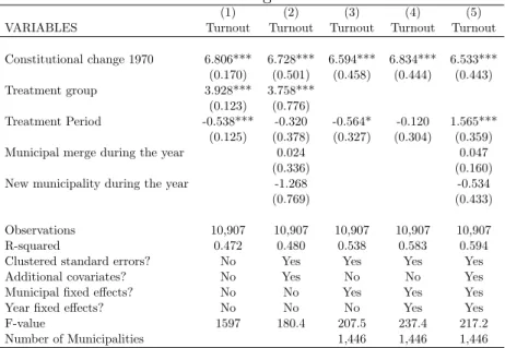
To begin with, table 3 indicates a strong first stage where the variable of interest, Constitutional change 1970, is statistically significant and the estimated parameter value is large. Note that the variable Constitutional change 1970 is an interaction variable between the variables Treatment group (equals 1 if the observation belongs to the Swedish subsample) and Treat-ment period (equals 1 if the observations belong to any year after 1970). The conclusion is that the reform package introduced in Sweden in 1970 did have an effect on voter participation. The estimated effect is robust for all specifications. This result is interesting and indicates that voter turnout will increase when the cost of voting is reduced. We may also conclude that we have a strong first stage by looking at the F-statistics from the first stage. In all specifications, the F-value exceeds the rule-of-thumb value of 10 and we may therefore conclude that the identifying assumption of instrument relevance is fulfilled. The constitutional reform in Sweden seems to increase voter turnout rate by approximately 6 percentage points.

(25)

Table 3: First Stage IV-estimates

(1) (2) (3) (4) (5)

VARIABLES Turnout Turnout Turnout Turnout Turnout

Constitutional change 1970 6.806*** 6.728*** 6.594*** 6.834*** 6.533*** (0.170) (0.501) (0.458) (0.444) (0.443) Treatment group 3.928*** 3.758*** (0.123) (0.776) Treatment Period -0.538*** -0.320 -0.564* -0.120 1.565*** (0.125) (0.378) (0.327) (0.304) (0.359)

Municipal merge during the year 0.024 0.047

(0.336) (0.160)

New municipality during the year -1.268 -0.534

(0.769) (0.433)

Observations 10,907 10,907 10,907 10,907 10,907

R-squared 0.472 0.480 0.538 0.583 0.594

F-value 1597 180.4 207.5 237.4 217.2

In table 4, the second stage IV regression outputs are presented. This IV specification should address the potential two-way causality between pol-icy outcomes and voter turnout. The voter turnout variable is statistically significant for all specifications and the estimate parameter value for the variable of interest is positive. There seem to be some negative correlation between a municipal merger and the local tax level. The inclusion of the merging dummy, however, does not seem to alter the point estimate of the turnout variable.

In summary, turnout rate seems have an effect on municipal tax rates. In the full model, the point estimates equal 0.04, which should be inter-preted as an increase of 0.04 percentage points in municipal tax rate when voter turnout increases one percentage point. This estimated effect is not enormous, although municipals seldom make drastic changes to municipal tax rates. If we consider the reduced form estimates presented in Appendix 3, which are equal to 0.258 in the fully specified model, the constitutional reform in Sweden increased the tax rate through voter turnout by 0.258 per-centage points. This increase constitutes approximately 6.5% of the total increase in tax rate during the time period for the Swedish subsample. In summary, the estimated effect should be considered economically significant.

(26)

Table 4: Second Stage IV-estimates

(1) (2) (3) (4) (5)

VARIABLES Taxrate Taxrate Taxrate Taxrate Taxrate

Turnout 0.066*** 0.119*** 0.315*** 0.037** 0.040**

(0.006) (0.033) (0.021) (0.016) (0.016)

Municipal merge during the year -0.639*** -0.093

(0.151) (0.059)

New municipality during the year -0.552 0.313**

(0.385) (0.152)

Observations 10,907 10,907 10,901 10,901 10,901

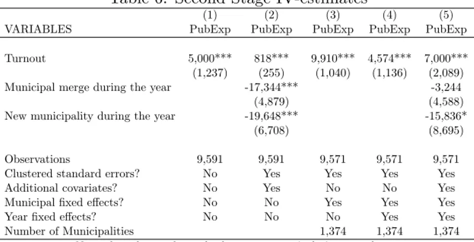
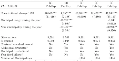
Let us turn to public expenditures. When performing the same operation using total public expenditures as dependent variable, as in table 5 below, the results are in line with those discussed above. Here, public expenditures are here expressed in thousands of USD in 2005 prices. Again, the OLS spec-ification is difficult to interpret since the point estimates are fairly variable for different specifications. Once again, however, I may conclude that there seems to be a statistically significant correlation between voter turnout and public expenditures when fixed effects are included together with additional covariates.

When examining the IV specification, the same pattern that was ex-hibited when tax rate was the dependent variable manifests itself. The magnitude of the point estimates is reduced when year fixed effects are in-cluded, but becomes larger after the inclusion of additional covariates. A one percentage points rise in turnout increases public expenditures by approxi-mately 7 000,000 USD in 2005 prices according to the fully specified model. If we relate this to the reduced form estimate in table 13 in Appendix 3, public expenditures increased by 47590,000 USD as a consequence of the re-form. This increase constitutes approximately 27 % of the total rise in public expenditures for Swedish municipalities for the time period 1967-1977. The estimated effect should therefore be considered economically significant.

(27)

Table 5: OLS estimates

(1) (2) (3) (4) (5)

VARIABLES PubExp PubExp PubExp PubExp PubExp

Turnout -5,997*** 789*** 5,613*** 1,755** 5,026***

(769) (257) (1,316) (796) (1,752)

Municipal merge during the year -17,219*** -2,920

(4,085) (4,570)

New municipality during the year -19,586*** -16,740**

(6,704) (7,862)

Observations 9,591 9,591 9,591 9,591 9,591

R-squared 0.006 0.948 0.016 0.071 0.294

Table 6: Second Stage IV-estimates

(1) (2) (3) (4) (5)

VARIABLES PubExp PubExp PubExp PubExp PubExp

Turnout 5,000*** 818*** 9,910*** 4,574*** 7,000***

(1,237) (255) (1,040) (1,136) (2,089)

Municipal merge during the year -17,344*** -3,244

(4,879) (4,588)

New municipality during the year -19,648*** -15,836*

(6,708) (8,695)

Observations 9,591 9,591 9,571 9,571 9,571

7.1 Party representation effects

As mentioned above, a potential political party effect might be an inter-mediate factor behind these results. The argument is that voter turnout will affect the share of votes for the various political parties and that the elected politicians will implement their preferred policy in accordance with the Citizen-Candidate model. To investigate this, I use the vote share for the right wing block as the dependent variable and then estimate the effect of turnout on vote share treating turnout as exogenous and endogenous. Note that all specifications in the results section hereafter are specified with

(28)

clustered standard errors as well with the inclusion of time and municipal fixed effects.

In the fully specified model, we have no statistically significant results in any specification and the point estimates are positive.48

Table 7: First and second stage and reduced form estimation; dependent variable is the vote share in % for the right wing block

(1) (2) (3) (4) (5) (6)

OLS OLS IV-Second stage IV-Second stage Reduced form Reduced form

VARIABLES RW.vote.share RW.vote.share RW.vote.share RW.vote.share RW.vote.share RW.vote.share

Turnout 0.006 0.009 0.124 0.116 (0.088) (0.090) (0.169) (0.167) Constitutional change 1970 0.908 0.832 (1.250) (1.214) Observations 3,701 3,701 3,244 3,244 3,701 3,701 R-squared 0.054 0.061 0.055 0.061 Number of Municipalities 1,439 1,439 982 982 1,439 1,439

Clustered standard errors? Yes Yes Yes Yes Yes Yes

Municipal fixed effects? Yes Yes Yes Yes Yes Yes

Year fixed effects? Yes Yes Yes Yes Yes Yes

Covariates? No Yes No Yes No Yes

Clustered standard errors in parentheses *** p<0.01 ** p<0.05 * p<0.1

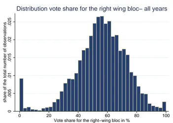
The sample used in this case, however, is somewhat problematic. In some municipalities, the right-wing block received no or very few votes. When studying the histogram below, it is clear that there are some distinct out-liers in the data that may drive the results presented above. I will therefore rerun the analysis dropping those observations where the right-wing block received less than 1 percent of the votes. I also drop the municipalities where the right-wing bloc received over 99 percent of the votes. The results are presented in the table below the histogram. For this specification, the esti-mated parameter values are still insignificant, but the point estimates now become negative.

48

Only election years are studied when analyzing the link between voter turnout and vote shares, so the sample size consequently becomes smaller.

(29)

0 .005 .01 .015 .02 .025

share of the total number of observations

0 20 40 60 80 100

Vote share for the right−wing bloc in %

Distribution vote share for the right wing bloc− all years

Table 8: First and second stage and reduced form estimation; dependent variable is the vote share in % for the right wing block. Outliers are deleted

(1) (2) (3) (4) (5) (6)

OLS OLS IV-Second stage IV-Second stage Reduced form Reduced form

VARIABLES RW.vote.share RW.vote.share RW.vote.share RW.vote.share RW.vote.share RW.vote.share

Turnout -0.068 -0.099* -0.064 -0.134 (0.060) (0.057) (0.136) (0.120) Constitutional change 1970 -0.471 -0.957 (1.028) (0.884) Observations 3,623 3,623 3,170 3,170 3,623 3,623 R-squared 0.118 0.126 0.117 0.126 Number of Municipalities 1,414 1,414 961 961 1,414 1,414

Clustered standard errors? Yes Yes Yes Yes Yes Yes

Municipal fixed effects? Yes Yes Yes Yes Yes Yes

Year fixed effects? Yes Yes Yes Yes Yes Yes

Covariates? No Yes No Yes No Yes

Clustered standard errors in parentheses *** p<0.01 ** p<0.05 * p<0.1

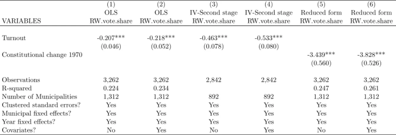
In some municipalities, local parties received a large share of the votes for various reasons and these parties are not always easy to categorize as either right-wing or left-wing. For example, they might be single-issue par-ties. To see if this will affect the results, I also run the same specification as in table 7, but drop those municipalities where local parties received more than 5 percentage points of the votes. This action renders the estimates sta-tistically significant and the point estimates negative and quite larger. This is displayed in table 9. In this specification we have a statistically significant effect for all specifications, both with and without included covariates.

There seems to be some evidence that a higher voter turnout rate is neg-ative for the vote share of right-wing parties when excluding municipalities with powerful local parties. The table below shows that for each percentage point of increase in voter turnout, the vote share for the right-wing block