Evaluation of Grasp-and-Extend Hand Dynamics and Intelligent Modeling of Grasp Hand Dynamics

V¨

aster˚

as, Sweden

Thesis for the Degree of Master of Science in Engineering - Robotics

30.0 credits

EVALUATION OF

GRASP-AND-EXTEND HAND

DYNAMICS AND INTELLIGENT

MODELING OF GRASP HAND

DYNAMICS

Josefine Gustafsson H¨

all

jhl13001@student.mdh.se

Examiner: Ning Xiong

M¨

alardalen University, V¨

aster˚

as, Sweden

Supervisor: Elaine ˚

Astrand

M¨

alardalen University, V¨

aster˚

as, Sweden

Table of Contents

6.4 From IMU data to angles . . . 12

7 Grasp-and-Extend Hand Dynamics 14 7.1 Differences Between Participants . . . 15

7.2 Differences Between Hands . . . 16

8 Implementation 17 8.1 Artificial Neural Network . . . 17

8.2 Radial Basis Function Neural Network . . . 18

8.3 Classification . . . 19

8.4 Prediction . . . 21

9 Assembly of Data Sets 23 9.1 Training Sets . . . 23 9.1.1 Classification . . . 23 9.1.2 Prediction . . . 23 9.2 Test Sets . . . 25 9.2.1 Classification . . . 25 9.2.2 Prediction . . . 25

10 Optimization and Network Design 27 10.1 Classification . . . 27

10.1.1 Result from classification training . . . 28

10.2 Prediction . . . 30

10.2.1 Raw Data with Change as Target Output . . . 32

10.2.2 Raw Data with Next Value as Target Output . . . 39

10.2.3 Angles with Change as Target Output . . . 40

10.2.4 Quaternions with Change as Target Output . . . 41

11 Result 42 11.1 Classification . . . 42

11.2 Prediction . . . 43

1

Introduction

This report presents the Master Thesis ”Evaluation of Grasp-and-Extend Hand Dynamics and Intelligent Modeling of Grasp Hand Dynamics” for which the work was performed at M¨alardalen University.

This theses focuses on the hand movements when a grip or an extension of the fingers is performed. Hand movements are controlled by the brain and if the brain gets damaged, there is a risk that these movements stop working. The brain can be damaged in many ways. One risk that the brain is exposed to is the experience of a stroke. A stroke occurs when there is a blood clot or an internal bleeding in the brain. This condition causes an area in the brain to obtain less oxygen than needed [1]. Strokes affect many people every year. Approximately 26500 people in Sweden experienced a stroke during 2016 [2]. There are many different ways in which the damage can be apparent. One of the more common consequences is loss of movement and, even more so, loss of hand movement. Many people never fully recover and when the loss of movement is too big, the patient can have difficulties to successfully part take in rehabilitation since they are not able to perform the necessary movements.

This thesis is part of the IEMI project at M¨alardalen University that is researching ways to improve stroke rehabilitation. One aspect that is researched is a way to use mental imagery as a tool for stroke rehabilitation. To use mental imagery, no actual movement need to take place [3,4]. When using this method the movement is imagined and in the project, EEG is recorded while mental imagery is used. The recording of mental imagery can be used to give feedback to the patient about it. This might be a way to improve the patients usage of mental imagery.

The hand movements are recorded to be used in this research in parallel to the mental imagery. Hand movements together with EEG data might be able to give more information about the per-formance and the improvement of the participants movements. This in turn could be used for feedback regarding the movement performances. If the movement dynamics can be found in the recorded hand data, it could be used to find the movements in real time and follow them. If the movements can be located in the data from the hand, the corresponding data from the EEG can be extracted and evaluated separately. If the movements can be predicted, it might be possible to determine whether a proceeding movement is continuing in the right way or if it looks different than the found dynamics. The thesis will examine the data recorded from the hands. It will also examine if and how artificial intelligence can be used to find these dynamics and locate movements.

2

Hypothesis

For this thesis, the hypothesis is that it is possible to model and predict movement dynamics of grip and finger extensions performed by a healthy or sick hand and that this can be done in real time as well as away from real time.

3

Problem Formulation

1. Can we model the movement dynamics of grasp and release hand movements from data mea-sured on both healthy participants and stroke survivors?

2. Can artificial intelligence be used to find patterns and predict behaviors in the data?

3. How can the model and the algorithms together give a stroke patient the tools to proceed with relearning to grasp and release objects?

used. Axel Forsdberg and colleagues used an IMU in a project aiming to make a bicycle balance[5]. The IMU was used to determine the lean angle and the lean angular velocity of the bicycle. Filters were used to process the raw data and the raw data was used to calculate the angle and the angular velocity. The method was successful in providing the angle and the angular velocity of the frame of the bicycle.

The IMUs that will be used in this thesis are of the kind MPU-9250. The IMUs contain an ac-celerometer, a gyroscope and a magnetometer [6]. All three components measure the movement in three axis. The three components that measure in three different axis produce in total nine signals to be evaluated. Together these signals give information about the different motions that the sensor experiences. The IMU sensors will be used to measure the movements of the hand when the participants close and open the hand.

The gyroscope measures rotational movement in the unit degrees/s[7]. The accelerometer measures the accelerations of the sensor in the unit m/s2 [8]. The magnetometer measures flux density or magnetic fields [9]. The magnetometers used in the IMUs measure in the unit µT [6].

A complementary filter can be used to calculate the angle and the angular velocity of the IMUs from the raw data obtained from the accelerometer and the gyroscope[5,10].

S. O. H. Madgwick and colleagues present in a study a method to calculate orientation from data obtained by IMUs[11]. Open source code on how to calculate euler angles from the raw data in MATLAB is evaluated [12].

4.2

Gesture Recognition

When training to regain mobility in a hand, a method for detecting the motion can be used to determine how the training is going. To do this, it is necessary to have a system that can describe and recognize the motion which, in this case, is a hand gesture. This system will use the data that have been recorded from the movements.

For handling the data and being able to give feedback to the user, the system will need informa-tion about the state of the movement. Gesture recogniinforma-tion is examined to see if there is a way to determine whether a movement is taking place and to predict the next step in the movement. There are different methods for grasping recognition such as Gaussian mixture models, hidden Markov models and time clustering. In the work of Ju and colleagues, these methods are tested by using a CyberGlove on one hand to obtain information about the hand movements[13]. 19 different joint angles are obtained, using angle sensors, by the glove and to test the gesture recognition, 13 different grasp gestures were chosen. When training, every grasp was repeated 11 times. Start and end points of the gestures were put on the data by pre-processing it. The algorithms, using different methods for calculations, were applied to the data and the results showed that the time

clustering algorithm outperformed the hidden Markov model and the Gaussian mixture model. It is stated that the reason the time clustering is better than the other two is the fact that more Euclidean distances are taken into consideration when comparing the data and the already created models to decide which gesture is occurring.

Gaussian mixture models are a form of unsupervised learning that is used to represent sub-populations of data point that lie within a bigger population by learning what sub-population the data points belong to [14]. The probability distributions over a number of observations can be described by using hidden Markov models. The models assume that the system evaluated fulfills a few properties, one of them being that at any time t, the state of the system is only dependent on the state that occurred at time t-1 [15]. There are many different clustering algorithms and they are used for many different things. A clustering algorithms divides a set of data into different clusters where the data points inside each cluster are near each other in appearance while at the same time far in appearance from data points in other clusters [16].

The paper written by S. S. Fels and G. E. Hinton describes a neural network that is trained to recognize hand gestures and link them to their corresponding words[17]. The information from the gestures is obtained by using a VPL Data-Glove and the total vocabulary consists of 203 word. On the VPL Data-Glove, there is one sensor on the back of the hand and two sensors (fiber optic transducers) for each finger. These sensors are used to measure the angles of the fingers and the hand. Within the vocabulary there are 66 root words and the words have several different endings. The authors, S. S. Fels and G. E. Hinton, suggest some improvement to be done, such as extending the vocabulary. With the vocabulary used, the system gives the wrong answer 1% of the times and no answer 5% of the times.

A convolutional neural network is similar to the standard multilayer neural network in that it contains at least one fully connected layer. Before the fully connected layers, there is also at least one convolutional layer [18].

H. Wang and colleagues present a way to recognize gestures from images and videos[19]. The frames are classified into two categories, gesture frames and transitional frames. There are differ-ent video sequences used for recognizing the gestures. One of them is RGB video sequences which contain information about colors and textures in the frames. The other is depth sequences which contain information about geometry and structures in the frames. Two different neural networks were used to handle the different video sequences, convolutional neural networks were used for the information obtained from the depth sequences and 3D ConvLSTM networks were used for the information obtained from the RGB sequences. The method was tested on a ChaLearn LAP ConGD Dataset, which is a gesture dataset, and the performance was evaluated using the Jaccard index [20]. The mean value of the relative overlap between the actual value and the predicted value is calculated when using the Jaccard index. The higher the Jaccard index is, the better is the result. The result obtained was approximately 0.5 which placed the method among the top performing methods when comparing it to other already existing methods.

Also in a paper written by A. Joshi and colleagues, a method that obtains gesture information from vision systems is presented[21]. The purpose for the paper is to develop an algorithm and a framework that can recognize gestures even if not the same subject is performing them every time. A hierarchical Bayesian neural network Is used to recognize gestures that differ between subjects. Three different datasets were used for training and all of them consisted of different gestures that were performed by different subjects. The method gave a more accurate result than choosing random gestures and the future work suggests testing of the framework in other domains and, from an input stream, localize and classify gestures.

A Radial Basis Function Neural Network can be used for classification and prediction of the coming data in a signal. A standard Radial Basis Function Neural Network consists of one input layer, one output layer and one hidden layer with radial basis functions [22]. The radial basis functions calculate a value from the distance between the outputs to center values that are stored in the

know whether any kind of training is successful, some kind of feedback is useful. When learning a new skill, such as a new language, feedback can be received by getting the correct usage of the language by either listening to, or reading, the language. When learning math, the feedback used for learning to solve a problem is the correct answer to the problem. Without this feedback, it is difficult to know if the answer obtained is the right one when the subjects knowledge is not enough to know the correct answer. The same phenomenon is present when learning a motor skill. It is easier to learn something if someone else is there helping with instructions on how to make it better and enhance the performance. In machine learning, many algorithms are given feedback to provide information of how well the system performed and how to change its behaviour to perform better next time. In the case of training a hand to grasp or release an object, sensors and data can be used to give an extra feedback other than the feedback from the person administering the rehabilitation. Small movements, aiming for a grasp or release, that are recorded over time can give information about the changes in the movements over time in a way that is difficult to manage by only looking at the hand. This information can give a more comprehensive picture of the state of the rehabilitation. Feedback that would tell the subject if the movement is occurring or not would be useful to give the subject more information about whether the progress is going in the right direction.

Visual feedback is used in the work described in a paper written by Liu and colleagues [25]. The work targets gait rehabilitation after a person has experienced a stroke causing loss of mobility in one leg. Walking is performed on a treadmill and the pelvis is supported by a manipulator that also helps with the movements. The treadmill is split in two, one for each foot, and they are controlled separately. Information from the treadmills is used to determine whether the participants weight is on them, and the information is transferred to simulate the same movement in a virtual scenario. The virtual scenario is used for the visual feedback. The paper concludes that the participant became more involved in and intuitive about the training when the visual feedback was used.

4.4

Related Work

In the work of Farshid Amirabdollahian and Michael L. Walters different hand gestures were clas-sified using Support Vector Machines [26]. The data was collected by a Myo armband [sic] that was gotten from Thalmic labs. The armband contains several sensors. There are 8 Electromyography electrodes and also accelerometers, gyroscopes and magnetometers. The armband communicates via Bluetooth 4. The test was setup by giving instructions of what gesture to perform to the participants. There were four motions of the hand to classify. The myoelectric signals obtained from the armband were used for classification. Different kernels were tested for the State Vector Machine, a linear kernel, a polynomial kernel and a Radial Basis Function kernel. The linear kernel produced the best accuracy during the training and the Radial Basis Function produced the worst. Tests were made using both 8 and 4 electrodes and the results were significantly better when 8 electrodes were used. The result for classifying the fists, witch were one of the gestures being classified and also the gesture with the highest classification accuracy was 97.60%. There is an ongoing new study that uses a higher sampling rate for collecting the data.

Muye Pang and colleagues presents a method for continuous prediction of a grasp motion [27]. In the study, sEMG signals were recorded using electrodes placed on the forearm. The method used is one of the conventional methods for predicting muscle movement, the Hill model. This model uses muscle activation levels and muscle length and shortening velocity to calculate the muscle force. The measurements were performed when the participants performed the movement without any load on the hand in form of the hand holding something. In the study there were two electrodes used to record data. There were some problems with predicting the movements and EMG signals can change depending on other motions than the one examined.

A method that uses an artificial neural network to classify where in a movement an arm is, is presented in a paper written by Tresadern and colleagues [28]. The movement is divided into different stages. The stages used are Reach/Retract, Grasp/Release and Manipulate. Depending on where in the movement the arm is located, the network gives the instruction for Functional Electrical Stimulation (FES) to the arm. The safety of the patient is considered and risks of hurt-ing the patients are taken into consideration when givhurt-ing the FES. The positions and movements of the arm were obtained by placing markers on the arm and reading them with a camera. For additional information and validation, Inertial Measurement Units located on the arm were used. The network was trained on three different movements, lifting a glass to the mouth, lifting a glass of the table and moving a plate sideways. When training on multiple movements, the third was the most difficult to classify in a correct way while the first one was the easiest. The network could generalize in a good way between lifting a glass to the mouth and lifting a glass from a table. Generalizations with the movement for moving a plate sideways was more difficult for the network. It was also difficult for the network to generalize between different participants performing the same movement.

Three models for linear regression are presented in a paper written by Rohafza and colleagues [29]. The paper examines the correlation between measured movements and the Wolf Motor Function Test which is a way to test the movements of an upper extremity. Data from the participants was collected both before and after the participants had been training. The models for linear regression were evaluated by letting them predict the result of the Wolf Motor Function Test and see how well they correlated. The paper concludes that the correlation was statistically significant. A high correlation points to the fact when describing the changes in a movement that has been trained, the method can contribute.

In a study by Kazemi and colleagues, the difference in grasping and twisting an object between healthy participants and participants that have experienced a stroke is evaluated [30]. Differences in coordination and force used were found between the two groups of participants. For the healthy participants the results pointed towards the fact that the grip force used linearly depended on the load torque that was put on the part to be twisted. One of the other results was that the force used to stop the twisting part from turning turn back automatically did not differ much between the healthy participants. For the participants that had experienced a stroke there were differences in both the affected hand and the unaffected hand. For example, the force used to keep the twisting part from turning back automatically was bigger than needed.

develop algorithms and then make it possible to test the algorithms on a few stroke patients. When performing the data collection, some problems were encountered. It turned out that some of the data in the obtained files were corrupted. This produced faulty time stamps in a manner that was different in different moments, making it difficult to fix all the data without making risky assumptions about them. Therefore the data attached to the faulty time stamps were removed, creating bigger time steps between some data packages. When examining one sensor at a time, it did not disturb the data a lot, but when attempting to match the data to get the relative value between the two sensors, a lot of the data was removed due to missing time stamps and the fact that most of the time the sensors send data with 4ms in between packages and sometimes with 5ms in between. Therefore, the focus in this theses will be on the data obtained from the sensor attached to the middle finger.

When recording data from the stroke patient the sensor on the hand was not able to send data. Therefore only data from the sensor on the middle finger was obtained.

6

Measurements

This section describes the method used to collect data from the test subjects. After that, the processing of the data is described. Data was collected from eight healthy participants and one stroke patient.

6.1

Experimental Setup

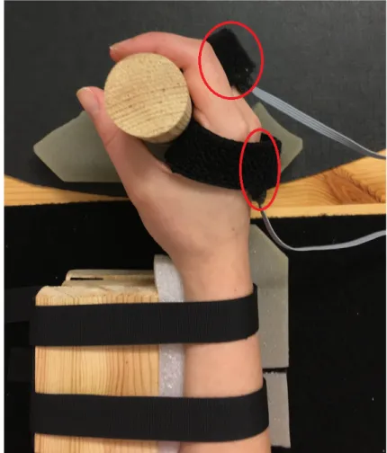
The measurements were obtained using two IMU sensors mounted on the measured hand. One of the sensors was located on the back of the hand and the other on the back of the middle finger. The sensors were marked so that they would be mounted the same way on all the test subjects. The test was performed while the subject was sitting on a chair looking at an instruction program on a screen. The arm of the measured hand was mounted on a table. The forearm was fastened with Velcro to a wooden construction, as seen in Figure1, to avoid unnecessary movements of the arm.

Figure 1: The setup of the hand and the sensors when the data was collected. The red circles show where the sensors are located.

The instruction program instructed the participant to either close the hand or extend the fingers. A response was given by sound when the movement should start. When the movement had been finished, it was held in place until another response was given telling the participant to relax the hand. There were 56 repetitions of grip movements and 56 repetitions of finger extensions per-formed in a random order during the test. When each of the responses to start a movement was given, a TTL pulse was sent to mark the time when the instruction was given.

remove the problematic data after the lines had been fixed were made. The process to handle the text files started with moving the sensor packages that had been put at the end of the last line in a new line below. The new file was saved under a different name. This method was developed when the only problems that had been seen were that either numbers were added to or removed from the time stamps. Later it was also noticed that numbers at some points were switched with each other which increased the complexity of the problem. After this new problem was discovered, the method changed to remove the entire lines where two data packages were located on the same line.

When the text file had been handled, the file was separated into two files containing the data from each of the sensors. In this process, empty lines and lines with only a couple of numbers which were present due to the recording problem described, were removed. After the data had been separated, the new files were evaluated and time stamps where the time stamp was smaller than the previous one or the same as the previous one as well as where the time stamp was a lot too big than the previous one were removed. The starting reference time is the first time stamp in the file. Therefore, the first value of the file will be removed when comparing the time stamps. The filtering of the data will also remove the start of the recorded data.

For each sensor, the different motions of the signals were extracted by using the TTL pulses that were set when the different instructions were given.

After the grip and finger extension parts of the data had been defined, the data sequences were stored separately to be used later.

6.3

Filtering

When the first processing of the data was completed it was evaluated whether filtering was needed. For removing some of the noise, a low pass filter was used.

6.3.1 Low-Pass filter

The signals produced by the IMUs are quite noisy. This proved to produce problems in the implementation phase when the raw data was used while examining the dynamics. Therefore, the signal was made to be softer. This was achieved by using a running average, shown in equation2.

y(t) = 1 2 ∗ b + 1 t+b X n=t−b x(n) (2)

b is the limit that decides how far from the current sample the average will be calculated. The resulting signal was not as noisy. If the solution is going to be used in real time a usual running average would not be useful. A running average takes points both from the past and the future when calculating the filtered signal. When running in real time, only past values can be examined, therefore equation3 was used when filtering the data.

y(t) = 1 b + 1 t X n=t−b x(n) (3)

6.4

From IMU data to angles

To calculate the angles from raw data to angles an open source code was used.

To use the open source code to calculate the angles of the signals, the data had to be restructured into data for accelerometer, gyroscope, magnetometer and time [12]. Before running the data in the program to calculate it to angles, it was run through a low pass filter like the one shown in equation3.

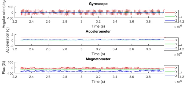
Figure2shows the raw data from the signal obtained from the sensor located on the left hand of subject 4.

Figure 2: Raw data from IMUs drawn by the open source code.

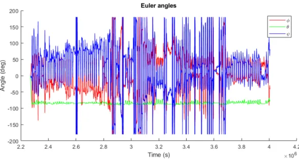
Figure3 shows the data when it has been recalculated to angles. As can be seen in the graphs, there are big, sudden differences in the angels. Even in the data that does not pass between 180 and -180 degrees, there are big differences.

The figure does not clearly state what vector contains the angles around which axis so this infor-mation is not known without making further investigations in the code. This does not produce a problem for training as long as the indices are not confused with each other.

After the raw data had been converted to angles, the angular velocity and the angular acceleration was calculated. This was done by subtracting the previous data value from the current value and dividing it with the change in time. The angular acceleration was calculated to be used as the target output in the training of the network. The problem that occurs is apparent when the values pass over +/-180 degrees. This created very big and fast differences in the data. This means that the calculated angular velocity and angular accelerations also have very big variations at times. This in turn means that the target output will be very large.

The open source code also provides a recalculation to quaternions that is shown in Figure4. The quaternion data do not contain the big changes in the data that the angle data does. Also when working with the quaternions, the quaternion velocities and accelerations were calculated. The method for these calculations were the same as when calculating the velocities and accelerations for the angles.

Figure 3: The Euler angles of the data after it had been calculated by the open source code.

7

Grasp-and-Extend Hand Dynamics

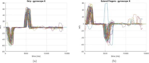
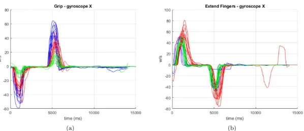
During the data collection, data from eight healthy subjects and one stroke patient were recorded. The data obtained from the stroke patient will be shown later in the report. After the data from the healthy subjects had been collected and processed, the dynamics of the hands were evaluated. When evaluating the raw data, all signals from the accelerometer, the gyroscope and the magne-tometer were considered. To not take up too much space in the report by showing all nine signals, the signal produced by the gyroscope on the x-axis was chosen. When looking at the angle data, one of the three euler angles are chosen and when looking at the quaternions, one of the four signals were chosen. Note that in the processing and implementation using the data, all signals will be used. That is, nine for the raw data, three for the euler angles and four for the quaternions. When looking at the raw IMU data it is clear that there are similarities between different repetitions of the same hand performing the same motions. Figure 5a show the grip and relax movements performed by the right hand of subject 4. The signals have been aligned, using the time stamps, to plot them over each other. The start of the x-axis represents where the signal for starting the movement was given to the participant. Figure5bshows the sequences when extending the fingers and relaxing as performed by the right hand of subject 4. Also in this case the start of the x-axis show where the signal was given to the participant to start the movement. The data in Figure5a

and5bhave been filtered with a running average as described by equation 3where b = 200.

(a) (b)

Figure 5: (a) shows the grip and relax motions placed on each other while (b) shows the extend fingers and relax motions placed over each other.

There are clear similarities between different repetitions. The clear exception is in one of the data signals in Figure5b, where the subject clearly did not perform the same movement as during the other repetitions. The similarities that are seen between different repetitions suggest that it should be possible to teach an algorithm to predict the data.

Also after calculating the angles, there are similarities between different repetitions of the same movement performed by the same hand. Figures6aand6bshow the hand dynamics of the grips and extend fingers separations performed by subject 4. The chosen signals show how the data looks when it is alternating over +/-180 degrees. There are similarities to be seen between the different signals also in the data that has been recalculated to angles.

Figure7show grips and finger extensions when the data has been recalculated to quaternions. The similarities between different repetitions are apparent in these graphs as well.

Although there are clear similarities over the general movement of the signals, there are also a quite wide range of values between the signals.

(a) (b)

Figure 6: (a) shows the grips performed by subject 4 while (b) shows the parts where the fingers were extended.

(a) (b)

Figure 7: (a) shows the grips performed by subject 4 while (b) shows the parts where the fingers were extended.

7.1

Differences Between Participants

When recording data from the same hand on different participants, the sensors were attached as similar as possible from one test to another. When looking at the same movement performed by the same hand but by different participants, there are more prominent differences in the data. Figure8a show ten grip sequences from subject 4 (blue), ten from subject 5 (red) and ten from subject 6 (green). The data from the gyroscopes x-axis show that the sensor moved with a higher velocity when attached to subject 4 and a lot slower when attached to subject 6.

Figure8bshows ten sequences each from subject 4, 5 and 6 when the fingers were extended. The color represents the same subjects as they did in figure8a. The data shows that the sensor moved faster when subject 5 was extending the fingers than when subjects 4 and 6 did so.

Although there are similarities between the data from different participants, as shown in the graphs, there are also more differences than already mentioned. One difference that was noticed was that before, after and in between movements, the data signals varies in different ways. For some subject there were also clear movements occurring at these times. One example of this that can be seen in Figure5bis in the red signals recorded from subject 5. During one of the signals, the data shows some kind of movement when all the other signals in the graphs are located closely to zero.

(a) (b)

Figure 8: (a) shows the different grips performed by subjects 4 (blue), 5 (red) and 6 (green) while (b) shows the extension of the fingers performed by subjects 4, 5 and 6.

The bigger differences observed when comparing data from different participants points to the fact that it might be more difficult to find a solution that can describe all participants than to only describe one.

7.2

Differences Between Hands

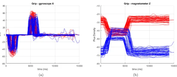
During the recording of data of different hands on the same person, the sensors were attached in a reflecting way between the hands. This was done so that there would be as little confusion as possible when examining the recorded data. In Figure9the data obtained from the left and right hand of subject 4 is shown. In the figure, grip and relax repetitions are shown. Figure9ashows the signals received from the gyroscopes recording on the x-axis and Figure9b shows the signals received from the magnetometers recording on the z-axis. The data from the right hand are shown in red in the graphs and the data from the left hand is shown in blue. It can be seen in Figure

9a that the signals are similar between the left and the right hand. With one of the difference being that the signals from the right hand have higher peaks. In Figure9bclear differences to the signals are seen. Although the signals are different, it is clear that with some modifications to the signal, such as flipping it around the x-axis and moving it down along the y-axis, they could be very similar to each other. Since it seems as if the signals could be made similar to each other by these methods, it suggests that the reason for the differences if the placement of the sensors and the fact that the movement is performed in a reflective manner between the hands. To be able to fully prove how the sensor placement and the reflective movements affect the data, more evaluations need to be performed.

Without changing the data in some way it would be difficult to teach a system to predict movements for both the left and the right hand without determining in some way witch hand is performing the movement.

(a) (b)

Figure 9: The data from the right hand is shown in red and from the left hand it is shown in blue. (a) shows the gyroscopes recording on the x-axis and (b) shows the magnetometers recording on the z-axis of the right and left hand of subject 4 and the unit of the flux density is µT.

8

Implementation

This section describes the implementation of the algorithms used in the thesis. There are two main problems to be looked at which are classification and prediction of the data. Prediction is important to determine whether the data sequence examined is part of a grasp and release movement and how the movements should progress next. The classification is needed to determine whether a movement is taking place or not. For the implementation an Artificial Neural Network (ANN) and a Radial Basis Function Neural Network (RBF-NN) was used. The following section first describes how the ANN was designed and then, how the RBF-NN was designed and based on the existing ANN. Finally, the standard RBF-NN and how it was used is described. The RBF-NN was chosen since the algorithm is useful for regression which is what is needed to learn to predict a system. The implementation was performed in MATLAB.

8.1

Artificial Neural Network

An Artificial Neural Network is a learning algorithm that, given an input, can be trained to give a correct output. The desired outputs need to be known for all data points before the network training is started. The ANN consists of several layers with at least one input layer and one output layer. It is also possible to have one or more hidden layers between the input and output layers. The layers are connected to each other and attached to all the connections there are weights that are being multiplied with the values when the values are sent between the layers. As the training is ongoing, the weights are updated to better the performance of the network. Each one of the data points in the data set used for training is sent through the network and the output layer gives the output from the data points when all the calculations are finished.

Initially, an Artificial Neural Network was chosen for predicting the grasping dynamics. The neural network was designed with an input layer, an output layer and a number of hidden layers. In the initial phase, different kinds of network designs were tested. Different kinds of activation functions were examined and different amounts of hidden layers were considered.

The input layer was designed differently depending on the training data. When the training data was obtained from the raw data from the IMU, the input layer consisted of nine nodes, one for each value from the IMU. When the training data consisted of the angles and angular velocities, the input layer consisted of 6 nodes, 3 for the angles and 3 for the angular velocities. When the quaternions were used, the input layer consisted of 8 nodes, 4 nodes for the quaternions and 4

nodes for the change of the quaternions.

Initially tests were made with both one and two hidden layers and the tests were made with the raw data provided by the IMUs. In the first tests performed the hidden layer consisted of nine hidden nodes. This number was chosen since both the input layer and the output layer consists of nine nodes when training was performed on the raw data. Eventually, the decision was made to use one hidden layer and test with different amounts of hidden nodes. Using only one hidden layer decreases the computation time during the training as there are fewer calculations made during one data points travel through the network and fewer weights to update.

The error of the network was calculated as: E = 1

2∗ X

(T argetOutput − output)2 (4)

The error is necessary to calculate to know how the network performs and to compare different networks to each other, the error function was changed to take the average of the combined squared errors instead of the combined square errors divided by two. This change was made to make it easier to compare the different networks to each other.

The weights are updated using backpropagation and the calculations are performed as described in the book Machine Learning [31]. To update the weights, the error terms of the output nodes first need to be calculated. There is one error term (δ) for each output node and the way to calculate them is shown in equation5where ˙a is the derivative of the activation function used in the output layer. The activation functions used in the networks will be further explained later in the section. δoutput= (T argetOutput − output) ∗ ˙a (5)

If the network contains more weights to update than between one layer and the output layer, these are the only error terms that need to be calculated. If there is a hidden layer where weights are connecting this hidden layer with a previous layer, the error terms for the hidden nodes in that layer also need to be calculated. To calculate these error terms, all of the weights going forward from the hidden node to an output node are multiplied by the error term of the output node it is connected to. These values are added together and multiplied with the derivative of the activation function in the hidden node. These error terms are calculated as shown in equation6.

δhidden= ˙a ∗

X

(weight ∗ δoutput) (6)

To calculate the value to add to the current weight, the error term for the node located at the end of the weight connection is multiplied with the value of the node in the beginning of the same weight connection. This value is then multiplied by the learning rate. These values are calculated as shown in equation 7 where l describes the learning rate, nodeprev describes the value in the

previous node that the weights is connected to and δnext describes the error term of the node at

the end of the connection.

∆weight = l ∗ δnext∗ nodeprev (7)

When this has been calculated the new weights can be calculated. Each new weight is calculated by adding the corresponding change to it. This is shown in equation8.

weight = weight + ∆weight (8)

8.2

Radial Basis Function Neural Network

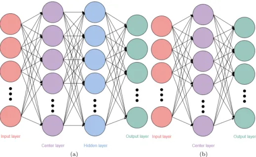
The RBF-NN used in the beginning was based on an ANN containing one hidden layer with an extra layer consisting of center nodes as shown in Figure10a.

The center nodes contain centers that are randomly extracted from the training data before the training is started. The values in the centers never change. When an input is given to the network, the Euler distances between the input and the centers are calculated. These distances show what

(a) (b)

Figure 10: (a) shows the network design when one center layer and one hidden layer was used. (b) shows the network design when one center layer and no hidden layer was used.

center nodes the input is close to and what center nodes are far away. This means that the net-work can update the weights depending on what should happen with the output when the input is close to which center nodes. These nodes give the network more information on how to behave depending on where in the data set the input is located. The distances are put into equation1to get the final value of the center node. The resulting value is higher, the closer the input is to the center. The k-value is calculated as 2*meandist. The meandist-value is the mean distance between the values in the center nodes. The k-value decides how fast the value of the center node decreases as the distance between the input values and the center node increases.

When the distance to the centers has been calculated, the outputs from the centers are sent into a hidden layer and the outputs from the hidden layer is sent to the output layer. Between the center layer and the hidden layer, as well as between the hidden layer and the output layer, weights are multiplied with the values. The weights are updated and the errors are calculated the same way as for the ANN. Also the same activation function is used.

Another design of the network that was tested was the standard RBF-NN. This network only uses an input layer, an output layer and one center nodes layer as shown in Figure 10b. This network sends the input values to the center nodes and calculates the distances to each of the centers and sends these values from the center layer to the output layer. There are weights to be updated between the center nodes and the output nodes. This design was tested to see the differ-ences between using a hidden layer or no hidden layer between the center layer and the output layer. The network was trained on different training sets to see its behaviour. The bigger the training set, the longer the computation time during the training.

Different training sessions will be further described and evaluated in section10.

8.3

Classification

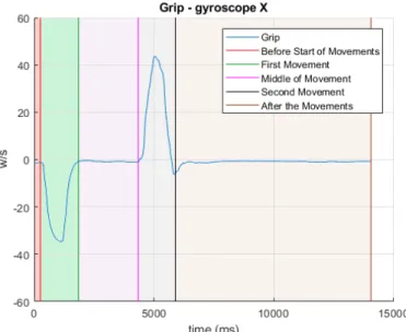
Part of the goal is to be able to classify different parts of the movements. To do this a network was designed to learn to perform the classifications. The classes for the training were constructed and assigned manually to the data. Five classes were defined for the grip motions and five were defined for the extension of the fingers. The classes were ”Before the Movement and After the Movement”,

”First Movement” (either grasp or extend), ”Between the movements” and ”Second Movement” (relaxing either the grasp or extend movement). Where the boundaries were set between the target output for the classification is shown in Figure11.

Figure 11: The manual classification of the data. The classes are located on the left of the vertical lines.

The target output is put together from the classes as a vector of (1x4) elements. The vector is defined as shown in Table1. Note that the classes ”Before Start of Movement” and ”After the Movements” are put together in the target output.

Before the Movement and After the Movement [1 0 0 0] First Movement [0 1 0 0] Between the Movements [0 0 1 0] Second Movement [0 0 0 1] Table 1: The target output for the classification training.

During the development of the network for classification, different designs were tested. In one ver-sion of the design, the network contained a summation layer where all the centers with the same classification was added together and divided by the number of centers that were containing the same classification. In this case there were weights between the centers and the summation nodes and between the summation nodes and the output. This design was not tested for the prediction network since the target output for the prediction is not as discretely separated as they are for the classification. Since all the centers in the center layer are different, it is unlikely that the target output will be equal between two different centers in the prediction center layer.

A second step of developing the classification network was to design it with a hidden layer after the center nodes layer as described above. In the classification network, the Sigmoid function, shown in equation 9, with its derivative, shown in equation 10, was used as the activation function. in the equations the variable o describes the output from the node before it is put into the activation function. This activation function was chosen since the target outputs for the different output nodes were set to either 0 or 1 for the different classes.

Finally, also as described above, the design of only an input layer, a center layer and an output layer was tested. Also in this case the Sigmoid function was used to calculate the final value of the output nodes.

values and the next value in the data divided by the change of time between the two values.

T argetOutputt=

(inputt+1− inputt)

timet+1− timet

(11) There was also a test made when the network trained on data where the target output was set to the next value of the signal.

The target output was defined for all data points before the training was started. This was done to simplify the process of mixing the data so that the data points in the training sets were not following each other chronologically in time. It also took away the calculations of setting the target output each time a new data sample was chosen. When training on the raw data, the output layer consisted of nine nodes, one for each data signal of the IMUs.

The purpose of mixing the data in the training sets was to avoid that the network continuously adapted to the current part of the training set.

The target output in the raw data becomes noisy since the signal is not completely smooth, even if it has been filtered. One attempt that was made to handle this was to filter the target output independently from the rest of the signal. The goal of this was to reduce the noise and have more consistency in the target output between data points that are close in time. The filter used for doing this was a running average that only looked to future target output values instead of past values in the data to only make the target output effected by future data. The filter used is shown in equation12. Another method that was tested was to filter the signal more from the beginning.

y(t) = 1 b + 1 t+b X n=t x(n) (12)

When training on the angles and angular velocities, the target output was set in the same way as for the raw data, but the target output was limited to the angular acceleration. Therefore, the output layer only contained three nodes during that training.

For the quaternion data, 4 target outputs were set in the data. These target outputs were defined as the 4 quaternion accelerations.

A few different activation functions were considered and the one used in the beginning was the Softsign function. The Softsign activation function looks like:

f (o) = o

1 + |o| (13)

˙

f (o) = 1

(1 + |o|)2 (14)

Where o is the output from the node. The Softsign activation function was chosen because of its properties. The output from the function varies between -1 and 1 and the output still has a small slope when it approaches -1 and 1. For using this activation function, the target output has to be less than or equal to the absolute value of 112_{. This activation function was used in the initial}

training on the raw data.

Since the angular acceleration at times exceed the absolute value of 1, the Softsign activation function would not be very efficient. Therefore, the Identity activation function was used. The Identity activation function does not change the value of the node and it is shown in equation15

and the derivative of the function is shown in equation16.

f (o) = o (15)

˙

f (o) = 1 (16)

The Identity activation function was also used when the network with the input and output layer connected by a center layer was trained. The Identity activation function is interesting to use since the values in the dynamics are not defined as any fixed values. Therefore it might be better to use the Identity activation function for the prediction even when training on raw data and quaternions. When considering this, it might be better to use the Identity function than the Softsign activation function.

1_{https://en.wikipedia.org/wiki/Activation function}

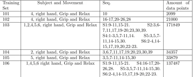
of one grip and relax movement performed by subject 4. This training set was created to test the classification implementation on a small training set to see if the resulting network would be able to classify the one signal after training. The full sequence contain much more data that belong to one of the classes. The over represented class is the one where no movement takes place, that is, the one called ”Before and After Movements”. To make the classes more evenly distributed and to decrease the training set a bit, the training set was limited to the data points 1-2100 of the entire grip and relax sequence. Training set 102 consists of 10 grip and relax repetitions performed by subject 4. Also in this set, the data points chosen were the first 2100 points in the sequences since subject 4 performed the motion in approximately the same time interval in all repetitions in the training set. Training set 103 uses 10 repetitions each from subjects 1, 2, 4, 5 and 6. The specific repetitions were chosen from the data depending on how they look. Repetitions that were clearly uncontrolled and differed from the standard dynamics were removed. In this case the entire signals were chosen in the training set and not just the 2100 first data points. This was due to the fact that different subjects performed the motions during different time intervals. Training set 104 was designed to train the classification of data obtained from subject 2 and training set 105 was designed to train the classification of data obtained from subject 5. Another version of training the classification on several subjects in the same training set is shown in training set 106.

Training Set

Subject and Movement Seq. Amount of

data points

101 4, right hand, Grip and Relax 10 2099

102 4, right hand, Grip and Relax 16-17,20-26,28 21000 103 1,2,4,5,6, right hand, Grip and Relax S1:9-11,15-21.

S2:3,6-7,11,17,19-20,23,30,39. S4:1-3,5,7-11,14. S5:3,5,7-11,14-15,30. S6:2-4,14-15,17,19,20,22-23.

171849

104 2, right hand, Grip and Relax 3,6,7,11,17,19,20,23,30,39 34357 105 5, right hand, Grip and Relax 3,5,7-11,14-15,30 33879 106 1,4,5,6 right hand, Grip and Relax S1:9-11,15-21.

S4:16-17,20-26,28. S5:3,5,7-11,14-15,30. S6:2-4,14-15,17,19-20,22-23.

137487

Table 2: Training sets used for classification of IMU raw data.

9.1.2 Prediction

For the prediction training the data sets were assembled to train different movements separately. The movements were separated in grips and finger extensions. After each grip or finger extension, the subject was instructed to relax the hand and return to a position in between the two motions.

Each motion was repeated 56 times during the data collection. When training to predict a move-ment the grip sequences were extracted. A grip sequence is defined as the motion of closing the hand without relaxing the fingers again and a finger extension sequence were defined as extending the fingers once without relaxing them again. The focus of the prediction was put on the grip sequences with the motivation to start the prediction training on one movement and evaluate the results.

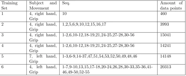
Table3shows the properties of the training sets that were assembled for predicting IMU raw data. All of the training sets are created from data that have been filtered with the low pass filter shown in equation3where b=200 except for training set 6 where b=400. Training set 1 is designed from one grip sequence performed by subject 4. The grip sequence contains 460 points and the target output has been calculated for all points. All data points in the sequence are used in the training set. Training set 1 is created to test the implementation of the prediction and see if the network would be able to predict one entire signal after training. Training set 2 is designed to train a network on several different grip sequences performed by Subject 4. 10 different sequences were chosen where some look similar but not all are similar to each other. All the data points in all the grip sequences were chosen for the training set and the amount of data points are shown in the tables. Training sets 3 and 4 consists of the data points contained in 40 grip sequences. The difference between them is that in set 4, the target output was filtered with a low pass filter seen in equation 12where b=20. During the testing of the network, most of the data used was from subject 4. The focus was put on data from one subjects to be able to compare networks and not have to consider differences produced by data from different subjects.

Training Set Subject and Movement Seq. Amount of data points 1 4, right hand, Grip 10 460 2 4, right hand, Grip 1,2,5,6,9,10,12,15,16,17 3993 3 4, right hand, Grip 1-2,6,10-12,18-19,21,24-25,27-28,30-56 15041 4 4, right hand, Grip 1-2,6,10-12,18-19,21,24-25,27-28,30-56 14241 5 7, left hand, Grip 1-3,6-9,14-37,47,51,54,53,52,50,49,48,46 14148 6 4, left hand, Grip 1-7,9-10,13,15,17-18,20-24,26,28,30-33,35-36,41-46,49-50,52-55 20313

Table 3: Training sets used for prediction of IMU raw data.

Another design for the training sets tested was to set the target output to the next value in the signals instead of to the change in the signals. Training set 201 described in Table4has the same design as training set 2. The only difference is how the target output is set.

Training Set Subject and Movement Seq. Amount of data points 201 4, right hand, Grip 1-2,5-6,9-10,12,15-17 3993

Table 4: Training sets used for prediction of IMU raw data,target output is next step. Table5 show the training sets for the training sessions where angles and quaternions were used. The definitions of the sequences that were made for the raw data are used to extract the sequences in the angle and quaternion data.

The test sets are designed to test the networks. Note that the data sequences in the test sets are different from the ones in the training sets.

9.2.1 Classification

Table6shows the test sets used for testing the networks that were trained for classification. Test set 1 was designed to test the result from training classification on grip and relax data collected from subject 4 which are kept in training set 102. Test set 2 was designed to test the classification accuracy of the network that have been trained on data from subject 2 (training set 104) and test set 3 was designed to test the network where the training set consisted of grip and relax movements performed by subject 5 (training set 105).

Test Set Subject and Movement Seq. Amounts of data points 1 4, right hand, Grip and Relax

1-15,18-19,27,29-56

172029 2 2, right hand, Grip and Relax

4-5,8-10,13- 14,18,21-22,26- 27,29,31,33-37,40-51,54-55

112262

3 5, right hand, Grip and Relax 1-2,6,12-13,16-29,31-33,35-52

136073

Table 6: Test sets for classification.

9.2.2 Prediction

Table7shows the test sets used to test the network trained for prediction. Test set 101 was used to test the performance of the network that trained on 10 different grips performed by subject 4 (training set 2). Test set 102 was designed to test the network where 40 grip sequences had been used for training (training set 3) and test set 103 was designed to test the network where 40 grip sequences were used in the training set and the target output was filtered (training set 4). Test set 104 was used to test the performance of the network trained on data from the left hand of subject 7 (training set 5). Test set 105 was designed to test the network that was trained on training set 6.

Test set 201 in Table8was designed to test the results from on the network that trained on training set 201. It is designed the same way as test set 101. The difference here is the target output of the test set.

In Table9the test sets to test the network trained with angle and quaternion data is shown. The test set is used to test the network that was trained on training set 302.

Test Set Subject and Movement Seq. Amounts of data points 101 4, right hand, Grip 3-4,7-8,11,13-14,18-56 17098 102 4, right hand, Grip 3-5,7-9,13-17,20,22-23,26,29 6050 103 4, right hand, Grip 3-5,7-9,13-17,20,22-23,26,29 5730 104 7, left hand, Grip 4-5,10-13,38-45,55-56 6429 105 4, left hand, Grip

8,11-12,14,16,19,25,27,29,34,37-40,47-48,51,56

9833

Table 7: Test sets for prediction.

Test Set Subject and Movement Seq. Amounts of data points 201 4, right hand, Grip 3-4,7-8,11,13-14,18-56 17098

Table 8: Test sets for prediction. The target output is the next value in the data.

Test Set Subject and Movement Seq. Amounts of data points 301 7, left hand, Grip 4-5,10-13,38-45,55-56 angel: 6445, quaternion: 6445.

is used is shown in equation1and further described in section8.

The error values were calculated as the mean error of all the data points in the training set. This does not take into consideration that the sets consisting of different data has a different amount of target outputs. The raw data has a target output for each of the data signals while the angle data has a target output for each of the angular accelerations and the quaternion data has a target output for each of the quaternion accelerations. This means that the training sets with raw data has 9 target outputs for each sample, the angle data have 3 target outputs and the quaternion data has 4 target outputs. Therefore it is necessary to recalculate these errors before being able to properly compare them to each other.

When the training sessions were stopped, they were stopped either at the end of an iteration through the training set or somewhere during the iteration of the training set. The weights used for testing were either the final weights obtained during the training or the weights that had been calculated when the training had produced the lowest error after an entire iteration through the training set. In the cases where the tests were performed online and the weights were updated throughout the test, the weights were reset to the saved weights between each tested grip sequence. This was done to see how much the mean error changed when in each movement sequence, the weights originated from the same values and were updated throughout the test.

The learning rate was set to 0.01 in most cases. In training sessions where it was not, such as training session 108 and 109 a learning rate of 0.005 was used and in training sessions 403 and 404 a learning rate of 0.0001 was used. The learning rate was changed due to the fact that the outputs of the network started to increase and eventually reached undefinable values.

10.1

Classification

Table10contains the training sessions for classification of training set 101. The training sessions contain different amounts of center nodes when there was no hidden layer and one session with 20 nodes in the hidden layer and 400 nodes in the center layer. The training sessions in Table10

were run to test the classification implementation on a small training set to see if the classification was successful in classifying data points in all classes and how well the data points were classified. Where 0 hidden nodes are noted in the tables, the network only consisted of an input layer, an output layer and a center layer.

When determining if the classification was correct or not, the determined class was chosen as the one with the maximum value in the output node. This means that even if it is not a big margin for the answer to be wrong, the classification will still be correct.

For classifying one grip sequence, training session 205 produced the best result for the training set. This is the sessions where the network contained a hidden layer with nodes in addition to the center layer. This design of the network makes the computation time for training much longer. To make this network larger when a larger training set is used would increase the computation time even

Training Session

Center Layer

Hidden Layer Activation Function

Iterations Max. Clas-sification (%) 201 40 nodes, k=2*13.0778 0 nodes Sigmoid 105 97.4738 202 100 nodes, k=2*17.6299 0 nodes Sigmoid 89190 98.9514 203 400 nodes, k=2*16.5614 0 nodes Sigmoid 54425 99.3804 204 1000 nodes, k=2*17.3011 0 nodes Sigmoid 34626 99.5234 205 400 nodes, k=2*17.7955 20 nodes Sigmoid 30981 99.7617

Table 10: The classification training sessions for training set 101.

more. The smallest network that still produced a result over 99% was produced during training session 203. Therefore, in the test with a bigger training set, the same design of the network will be used. Although this was the decision made, it is worth noting that the networks were trained for a different amount of iterations through the training set.

Table11shows the resulting network when the training was performed on several grip and relax repetitions performed by the same subject. The training sets used in these sessions are described in section9 and the training set index are shown in Table11. The table shows that the training accuracy of all the training sessions is over 90%.

Training Sessions Center Layer Hidden Layer Activation Function Training Set

Iterations Max. Clas-sification (%) 301 400 nodes, k=2*18.1310 0 nodes Sigmoid 102 1202 95.0236 302 400 nodes, k=2*21.2767 0 nodes Sigmoid 104 7298 96.4053 303 400 nodes, k=2*13.7199 0 nodes Sigmoid 105 7498 97.8836 304 1000 nodes, k=2*27.1634 0 nodes Sigmoid 103 1898 95.9394 305 1000 nodes, k=2*26.5147 0 nodes Sigmoid 106 1471 96.5778

Table 11: The training sessions for classification.

10.1.1 Result from classification training

Figure 12 shows the classification of the signal used in training sessions 201, 203 and 205. The signal used in the testing is the same signal that was used in the training set. The green dots show where the classification was successful and the red dots show where the classification failed. The vertical lines show where the classes in the signal changed. It is clear that the problem with classifying the signals occur where the classes change in the signal.

After training the network on several signals performed by the same hand on subject 4, the result from testing the network on a test set is shown in Table12. The mean classification accuracy of all data points in the test set was 90,56%. The median accuracy was calculated by looking at the accuracy of one repetition of the grips and relax movement at a time. The median accuracy is

(c)

Figure 12: The classification of the signal that was in the training set during training sessions 201, 203 and 205.

higher than the mean accuracy, this is due to the fact that one of the grip and relax repetitions had a low accuracy.

Test Set Training Session Classification Accuracy (%) Median (%)

1 301 90.5621 94.6717

2 302 65.2686 75.1526

3 303 75.1538 88.0455

Table 12: The result from testing a network on different test sets.

In the table, also the result from classifying several grip and relax sequences performed by subjects 2 and 5 can be seen. There are a much lower classification accuracy for the test on subject 2 and 5 than for subject 4. Test set 1 contains data from subject 4, test set 2 contained data from subject 2 and test set 3 contains data from subject 5. The design of the networks in the training sessions and the training sets used can be seen in Table11.

Figure13ashow the classification of test set 1. In the figure it can be seen that the most classifi-cation mistakes made are made before the movements has started and after the movements have stopped. Figure13bshows the classification of the grip sequences performed by subject 2 (test set 2). Note that for subject 2, the movement in the data looks different than in the data collected from subjects 4 and 5. This will be further discussed in section13. The classification for subject 2 did not perform very well on the test set. What can be seen in the figure is that there are a lot of smaller movements between the two main movements. These smaller movements were not present in the training set. Figure13cshows the classification performed on the test set designed for subject 5 (test set 3). The most classification mistakes for classifying subject 5 was also made in between the movements and before and after the movements.

(a) (b)

(c)

Figure 13: The green points show where the classification was successful and the red points show where the mistakes are made. The vertical lines show where in the data the class changed. (a) shows the classification of the test set obtained from data from subject 4. (b) shows the classification of the test set obtained from data from subject 2 and (c) shows the classification of the test set obtained from data from subject 5.

When multiple subjects were used for classifications of the movements of the right hand, the differing data of subject 2 was included. The classification training still produced a good training result but when the testing was performed, the accuracy was not very high and there were also mistakes made in the classes where the movements occurred. Therefore a classification training session where subject 2 was removed was designed. Tests of the classification training performed on several subjects will be shown in section11where the training set used consists of 40 grip and relax sequences each performed by four subjects.

10.2

Prediction

The training sessions are separated into different tables depending on the training set or type of training sets used. Table13show the training sessions that used training set 1 for training. These training sessions were used to find an effective training method by training on a small training set. When comparing the networks, different amounts of center nodes and different amounts of hidden nodes were used. Where it is shown that 0 hidden nodes were used, the only hidden layer used was the center layer. The training sessions were stopped after 105 _{iterations and compared after that.}

The sessions could have been run longer and lower the errors further, they were stopped so that the training time would not be too long. They were stopped after an equal number of iterations to be able to compare the errors at the same point of training. Depending on the size of the network, the computation time for the training differed a lot.

k=1 7 40 nodes, k=1 20 nodes Identity 105 0.0032 8 100 nodes, k=1 20 nodes Softsign 105 _0.0012

Table 13: The training sessions for training on training set 1.

The training session that produced the lowest error in Table13was session 6. This session uses 400 center nodes for a training set of 460 data points. This means that almost every data point is a center node. To use the same proportion of center nodes to data points in bigger training sets would increase the computation time significantly. The design of the network in training session 6 contains a hidden layer. This layer also adds to the computation time and to increase this layer also increases the computation time. When comparing training sessions 1 and 4 it can be seen that the results were better for session 4. The difference is that in training session 4, the k value is calculated as k = 2*meandist in the radial basis function. Therefore when training on different, bigger training sets, the k value will be calculated the same way.

The training sessions used for training on training set 2 were designed based on the results obtained from training on the small training set. When designing the training sessions shown in Table14, at first the sessions got the amount of center nodes and hidden nodes proportional to the data points in the training set roughly the same way as it is proportional to the data points in Table

13. The amount of center nodes was a quarter of the amount of data points (based on training session 4) and the amount of hidden nodes, when they were used, was a twentieth of the amount of data points (based on training session 6). In Table14other training sessions are described where the training sets contain more than one grip sequence. To reduce the computation time for the training when the size of the training sets increased, the amount of center nodes were set to a tenth of the amount of data points.

Table 15 describe the training sessions designed to train networks on IMU data that have been recalculated to angles and quaternions. Training sessions 401 and 402 uses a training set that only consists of one movement. A training set consisting of 40 grip sequences was used for training sessions 403 and 404. It can be seen when comparing training sessions 401 and 403, where the angle data was used, that the error increased a lot. When comparing training sessions 402 and 404, where the quaternion data was used, there was not as big of a difference between the errors. It is also notable that when bigger training sets were used, the networks were not trained for as many iterations through the entire training set.

The prediction of the data was performed on different kinds of signals and target outputs to test different methods for performing the prediction.

Training Session Center Layer Hidden Layer Activation Function Training Set

Iterations Min. error 101 998 nodes, k=2*23.4457 200 nodes Identity 2 1159 1.5280 ∗ 10−4 102 998 nodes, k=2*23.2042 200 nodes Softsign 2 1147 1.2044 ∗ 10−4 103 998 nodes, k=2*23.2733 0 nodes Identity 2 18905 1.1601 ∗ 10−4 104 1504 nodes, k=2*25.5704 0 nodes Identity 3 871 0.0019 105 998 nodes, k=2*23.3463 0 nodes Identity 201 59964 0.2271 106 1429 nodes, k=2*25.6836 0 nodes Identity 4 10998 0.0013 107 1415 nodes, k=2*17.6291 0 nodes Identity 5 9598 0.0015 108 3537 nodes, k=2*17.6722 0 nodes Identity 5 7351 0.0015 109 2031 nodes, k=2*15.8823 0 nodes Identity 6 4562 2.5355 ∗ 10−4

Table 14: The training sessions for prediction training on more than 1 repetition of a grip move-ment.

Training Session

Center Layer Hidden Layer

Activation Function

Training Set

Iterations Min. error

401 92 nodes,

k=2*4.6329

0 nodes Identity 301, angle 105 3.9193 ∗ 10−5

402 92 nodes, k=2*0.0394 0 nodes Identity 301, quater-nion 105 _{2.3044 ∗ 10}−9 403 1419 nodes, k=2*217.5819

0 nodes Identity 302, angle 14188 2.2756 404 1419 nodes, k=2*0.0766 0 nodes Identity 302, quater-nion 14430 4.9276 ∗ 10−8

Table 15: The training sessions for prediction training on angle and quaternion data.

10.2.1 Raw Data with Change as Target Output

One of the methods used to train the prediction of the signal used the change of the signals as the target output. Different training sets were used to test the training in different setups. First, only one repetition of the grip movement was used to see if the network was able to learn the dynamics of the signals and later training sets with several signals were examined. Although the graphs shown in this section are not over all signals produced by the IMU, all nine signals produced by the IMU are used in the training.

An example of the resulting predictions for training set 1 can be seen in Figure 14and 15. The plots shown are selected values of the grip sequence used for training on training set 1 and their prediction by the network. The signals chosen were the Accelerometer Y, Accelerometer Z, Gy-roscope X and Magnetometer Y. The Accelerometer Z signal was chosen because it had the most spread between the real signal and the predicted ones. The Accelerometer Y signal was chosen to show that not all Accelerometer signals were as problematic as the Z one. The Gyroscope X and Magnetometer Y signals were chosen to show one each of the gyroscope and magnetometer signals.