Automated Segmentation of the Meniscus

INOM TEKNIKOMRÅDET

EXAMENSARBETE

MEDICINSK TEKNIK

OCH HUVUDOMRÅDET

TEKNISK FYSIK,

AVANCERAD NIVÅ, 30 HP

,

STOCKHOLM SVERIGE 2017

Automated Segmentation of

the Meniscus

FELICIA ALDRIN

KTH

TRITA FYS 2017:43 ISSN 0280-316X

ISRN KTH/FYS/--17:43—SE

Abstract

3D segmentation of tissues in the knee joint helps to visualise lesions and defor-mations, enabling computer-aided diagnosis and treatment planning of patients with knee problems. Manual segmentation is, however, time-consuming and sub-ject to inter-rater variability, creating a natural desire for methods enabling au-tomated segmentation. There is a range of segmentation methods reported with good results for tissues in the human body. Some tissues do however still remain challenging to segment, such as the relatively small structure of the menisci in the knee. The development of machine learning in recent years has dramatically improved automated image segmentation and classification tasks[1], making it a natural choice for the more challenging menisci segmentation. In this thesis, two fully automated machine learning segmentation methods are implemented and compared for segmentation of the menisci, namely Random Forest based on Haar-like features and the deep learning method 2D UNet fully convolutional network (FCN). Both methods were tested and compared for segmentation of 18 menisci from 3D magnetic resonance (MR) images. The 2D UNet cascade showed superior results compared to the Random Forest for segmentation of the menisci, with a mean Dice Similarity Coefficient (DSC) of 75.3% compared to 54.4%.

Furthermore, 2D UNet cascade was also tested on additional 28 subjects for single- and multi-class segmentation of distal femur and articular cartilage from 3D MR images. The single-class 2D UNet cascade gave marginally better results compared to the multi-class segmentation with a mean DSC of 95.3% for distal femur and 71.7% for the articular cartilage.

With limited training data, the proposed 2D UNet cascade segmentation method shows promising results for all three tissues. Based on the results pre-sented in this thesis, future work is proposed to focus on the 2D UNet cascade algorithm. Further training on more data as well as dividing images for training in separate networks based on properties of the images is suggested.

Keywords

MRI, segmentation, classification, Random Forest, Deep Learning, Convolu-tional Network, knee, meniscus, distal femur, articular cartilage

Sammanfattning

3D segmentering av v¨avnader i kn¨aleden kan visualisera skador och deforma-tioner och m¨ojligg¨ora bland annat datorunderst¨odd diagnostisering och planer-ing av behandlplaner-ingsalternativ f¨or patienter med kn¨aproblem. Manuell segmenter-ing ¨ar dock tidskr¨avande och kan ge varierande resultat beroende p˚a vem som g¨or segmenteringen. F¨or att ˚astadkomma j¨amnare och mera p˚alitliga segmenterings-resultat ¨ar det ¨onskv¨art att automatisera segmenterings-processen. Det finns en rad olika automatiserade segmenterings-metoder rapporterade i litteraturen till¨ampbara p˚a v¨avnader i m¨anniskokroppen. Vissa v¨avnader ¨ar dock fort-farande en utmaning att segmentera, som till exempel de relativt sm˚a meniskerna i kn¨aet. Utvecklingen av maskininl¨arning de senaste ˚aren har drastiskt f¨orb¨attrat automatiserad segmentering och klassificering av bilder[1], vilket gjorde mask-ininl¨arning till ett naturligt val av segmenteringsmetod i detta arbete. Im-plementerade och testade i detta arbete ¨ar tv˚a fullt automatiserade segmenter-ingsmetoder, Random Forest baserad p˚a Haar-like egenskaper samt ett 2D UNet fully concolutional networks (FSN). B˚ada metoderna testades och j¨amf¨ordes f¨or segmentering av meniskerna i 3D magnetresonans-bilder. 2D UNet kaskaden gav ¨overl¨agsna resultat i j¨amf¨orelse med resultaten fr˚an segmenteringen med Random Forest. Genomsnittning Dice likhets-koefficient (DSC) blev 75.3% f¨or 2D UNet kaskad och 54.4% f¨or Random Forest.

2D UNet kaskaden testades f¨or ytterligare 28 fall f¨or singel- och multi-klass segmentering av distala l˚arbenet och distala l˚arbensbrosket i MR-bilder. 2D UNet kaskaden med singel-klassificering gav n˚agot b¨attre resultat ¨an multi-klassificeringen med en genomsnittlig Dice-koefficient p˚a 95.3% f¨or distala l˚arbenet och 71.7% f¨or distala l˚arbensbrosket.

Den f¨oreslagna segmenteringsmetoden med 2D UNet-kaskaden gav, med begr¨ansad data f¨or tr¨aning av n¨atverken, lovande resultat f¨or alla tre v¨avnader den testats f¨or. Baserat p˚a resultaten presenterade i denna rapport, s˚a f¨oresl˚as framtida arbeta att fokusera p˚a segmenteringsmetoden 2D UNet-kaskad. F¨or att f¨orb¨attra algoritmen b¨or vidare tr¨aning av n¨atverken genomf¨oras med mer tr¨anings-data. Data kan ocks˚a delas upp och tr¨anas i olika n¨atverk baserat p˚a olika bildegenskaper.

Nyckelord

MR, segmentering, klassificering, Random Forest, Deep Learning, Convolutional Network, kn¨a, menisk, distala femur, ledbrosk

Acknowledgments

The work in this thesis was conducted in collaboration with Episurf Medical AB. The work would not have been made possible without my supervisor Chunliang Wang at the School of Technology and Healthy (STH). Thank you for giving me invaluable guidance, support and motivation throughout the work of my thesis. In addition, I would like to thank Episurf for introducing me to the topic of this thesis and giving me the opportunity to work in an up and coming field.

Abbreviation Meaning

AI Artificial intelligence ANN Artificial Neural Network ASM Active Shape Model CAD Computer Aided Diagnosis CNN Convolutional Neural Networks

CT Computed Tomography

DBN Deep Belief Networks

DRF Discriminative Random Field DSC Dice Similarity Coefficient ELM Extreme Learning Machine LM Lateral Meniscus

MLP Multi Layer Perceptron

MM Medial Meniscus

MO Morphological Operations MR Magnetic Resonance

MRI Magnetic Resonance Imaging NMR Nuclear Magnetic Resonance OA Osteoarthritis

PD Proton Density

RF Radio Frequency

RNN Recurrent Neural Networks SAE Stacked Auto-Encoders SE Structuring Element SENSE SENSitivity Encoding SLP Single Layer Perceptron

SM Shape Model

SNR Signal to Noise Ratio

SPAIR SPectral Attenuated Inversion Recovery SSM Statistical Shape Model

SVM Support Vector Machines

VIBE Volumetric Interpolated Breath-Hold WATSc WATer Selective

WE Water Excitation

Contents

1 Introduction 1

2 Theoretical Background 3

2.1 The menisci . . . 3

2.1.1 Menisci Anatomy and Biomechanics . . . 3

2.1.2 Menisci Pathology . . . 4

2.1.3 MRI of the Menisci . . . 4

2.1.4 Challenges in menisci segmentation . . . 7

2.2 Magnetic Resonance Imaging . . . 9

2.2.1 Nuclear Magnetic Resonance . . . 9

2.2.2 Radio frequency pulses & Relaxation Times . . . 10

2.2.3 Signal . . . 11

2.2.4 Magnetic gradient fields . . . 11

2.2.5 Image Contrast . . . 11 2.2.6 2D vs. 3D imaging . . . 12 2.2.7 MRI Artifacts . . . 12 2.3 Segmentation . . . 13 2.3.1 Manual Segmentation . . . 13 2.3.2 Thresholding . . . 13

2.3.3 Binary Morphological Operations . . . 14

2.3.4 Region Growing . . . 15

2.3.5 Machine Learning . . . 16

2.3.6 Random Forest Classification . . . 16

2.3.7 Deep Learning and Artifical Neural Networks . . . 18

2.4 Review of Previous Work . . . 22

2.4.1 Datasets . . . 23

2.4.2 Pre-processing . . . 24

2.4.3 Segmentation methods . . . 24

2.4.4 Post-processing . . . 25

2.4.5 Validation and Results . . . 25

3 Method and Material 27 3.1 Image & Subject data . . . 27

3.2 Manual segmentation technique . . . 28

3.3 Pre-processing . . . 30

3.4 Random Forest Segmentation . . . 30

3.5 Deep Learning . . . 31

4 Results 35 4.1 Menisci . . . 35 4.2 Femur Bone & Articular Cartilage . . . 38

5 Discussion and Conclusion 43

6 Future Work 47

Bibliography 49

Appendices

Chapter 1

Introduction

Osteoarthritis is the most common joint disorder worldwide, with knee and hip osteoarthritis being the two joints associated with the greatest social cost and disability compared to other joints[3]. In a study of 31,516 knee arthroscopies, cartilage lesions were found in 63% of the subjects and other knee joint lesions in 43% of the subjects, with medial meniscus lesions being the most common[4]. Magnetic resonance imaging (MRI) has become the preferred method for non-invasive evaluation and assessment of the knee due to its high accuracy rate ranging from 92% to 98%[5]. 3D segmentation (the process of separating and classifying an object in an image) of structures in the knee joint from MR im-ages helps to visualise the overall state of the knee and enables computer-aided diagnosis as well as treatment planning. Manual segmentation of the knee joint is, however, a challenging and time-consuming task, making automatic segmen-tation desirable. There are many published results for automated bone and articular cartilage segmentation available, however, the results for automated menisci segmentation are more limited. The menisci are relatively small struc-tures in the knee, making them challenging to segment automatically. The segmentation task becomes even more challenging if there are signal changes within the tissue in the image, normally caused by lesions or ruptures in the menisci.

There are many segmentation methods reported, both semi- and fully au-tomated. Semi-automated methods require the user to, for example, pre-define grey level values or seed points in order to enable segmentation. Such methods are limited due to the manpower required, the varying outcome depending on the pre-defined values as well as difficulties to segment complex structures in images with a wide range of pixel values.[6] More complex segmentation meth-ods, such as atlas or deformable model based segmentations, show limitations in segmenting more complex structures with different shape and size.[6]

Machine learning, a subset of artificial intelligence (AI), is the concept of computers learning how to perform tasks or solve problems specified by the user. In recent years, machine learning has been developed and applied to more and more complex problems across different industries and is has drastically

improved automated segmentation and classification tasks.[1] The recent devel-opment in machine learning is thanks to the drastically improved computing power, as well as the vast amount of data available.

Based on existing segmentation software and algorithms, the aim of the work in this thesis is to implement and test different methods for automated segmentation of the menisci from 3D MR images in knees showing different grades of joint degeneration. The project is limited to two machine learning approaches, Random Forest and Deep Learning, using a 3D T1 VIBE WE1 -protocol (or similar). This project is part of a larger effort to segment all the main structures in the knee joint. If time allows, other structures in the knee will be segmented using the same methods as implemented for the menisci.

Chapter 2

Theoretical Background

2.1

The menisci

2.1.1

Menisci Anatomy and Biomechanics

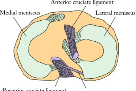
The menisci play an important role in the knee joint. The menisci comprise mainly of water (75%) and fibrous cartilage and they have few mobile protons.[7, 8, 9] The composition of materials, the geometry and the attachments of the menisci help absorbing shocks and distribute load over a larger area in the knee.[7] The two crescent-shaped menisci are found on the medial and lateral sides in the knee between the plateau of the tibial bone and the two epicondyles of the distal femur, see figure 2.1. The top surfaces of the menisci are concave, following the bone surfaces of the femoral epicondyles, while the bottom surfaces of the menisci are flat, following the shape of the tibial plateau.

Figure 2.1: Schematic illustration of the menisci on top of the tibial plateau.

2.1.2

Menisci Pathology

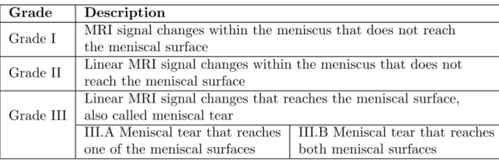
MR imaging is the golden standard for noninvasive evaluation and assessment of injured or degenerated menisci with an accuracy rate ranging from 92% to 98%.[9, 5] There are several grading systems available for menisci pathology, easily causing confusion amongst doctors. With the aim to create a universal scientific language for arthroscopic surgeons, ISAKOS1and ESSKA2published a report in 2006[9] presenting a standardized international meniscal grading sys-tem that describes abnormal signal changes within the menisci[7, 9]. A summary of the grading system is presented in Table 2.1.

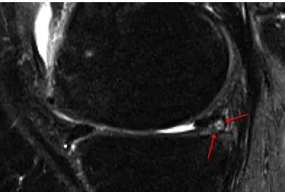
In a study by Englund et al. [11] meniscal damage was found to be present in 38% of the knees of subjects with frequent knee pain, and in 28% of the knee of subjects with no knee pain. Making quantitative analysis of the menisci size, volume and position helps not only in making a damage assessment of the menisci, but also to understand how menisci degeneration is associated with knee osteoarthritis.[12] Wirth et al. [13] shows that the medial meniscus in knees with osteoarthritis tend to be thicker, have greater size and increased extrusion compared to menisci in non-osteoarthritis knees. In Figure 2.6 a degenerated meniscus is depicted with the MRI signal changes pointed out with red arrows.

Grade Description

Grade I MRI signal changes within the meniscus that does not reach the meniscal surface

Grade II Linear MRI signal changes within the meniscus that does not reach the meniscal surface

Grade III

Linear MRI signal changes that reaches the meniscal surface, also called meniscal tear

III.A Meniscal tear that reaches one of the meniscal surfaces

III.B Meniscal tear that reaches both meniscal surfaces

Table 2.1: Grading of meniscal lesions.

2.1.3

MRI of the Menisci

As mentioned in Section 2.1.2 above, MRI can be used to accurately assess the menisci. However, it is important to use the appropriate MR protocol as well as imaging planes that enable the visualisation of the menisci and any pathological changes. The menisci can be imaged in 2D or 3D, where 2D images give a good diagnostic value of the menisci, while with 3D images makes it possible to obtain morphological and anatomical information useful in the segmentation of the menisci.

1_{The International Society of Arthroscopy, Knee Surgery and Orthopaedic Sports Medicine} 2_{The European Society of Sports Traumatology, Knee Surgery and Arthroscopy}

Imaging Planes

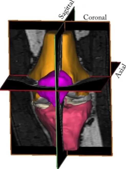
MR images of the knee are normally obtained in three orthogonal planes, sagittal (sag), coronal (cor) or axial/transversal (ax/tra), see Figure 2.2. The menisci are relatively small structures, especially the thickness in the axial direction. Hence, the menisci are best visualised in the sagittal and coronal imaging planes[5]. The lateral meniscus is depicted in the sagittal plane in Figure 2.3, a T2 weighted 2D image. In Figure 2.4, both menisci are depicted in the coronal plane in a PD-weighted 2D image with fat saturation (FS). To visualise and assess the menisci in the axial plane, there need to be a sufficient number of thin image slices in that direction. In Figure 2.5, the menisci are depicted in three orthogonal planes in a 3D WATSc SENSE sequence. The menisci in all MR images are depicted as low-intensity structures between the femoral and tibial bones and pointed out with red arrows in both images.

Figure 2.2: The knee joint depicted from the anterior side with the three orthogonal imaging planes market out.

Figure 2.3: A T2-weighted 2D MR image of the knee joint in the sagittal plane, with the lateral meniscus is pointed out with red arrows. The image to the right indicates the position of the image slice in the knee joint.

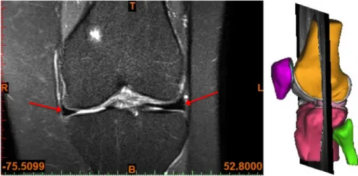
Figure 2.4: A PD FS 2D MR image of the knee joint in the coronal plane, with both menisci pointed out with red arrows. The image to the right indicates the position of the image slice in the knee joint.

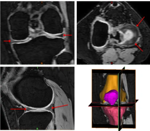
Figure 2.5: The menisci pointed out with red arrows in all three orthogonal planes in a 3D WATSc SENSE sequence. Top left: coronal view. Top right: axial view. Bottom left: sagittal view. Bottom right: 3D view.

2.1.4

Challenges in menisci segmentation

There are many challenges with both manual and automatic segmentation of MR images. There is an obvious desire to overcome these challenges with au-tomatic segmentation methods, and it has already been done for many tissues and applications. Nonetheless, there are still many challenges to overcome, and it is often necessary for a visual check of the segmentation by a human eye to confirm its accuracy. In this section, an overview of the main challenges with image segmentation of MR images are presented.

Image quality and artifacts

The image quality and signal intensity can differ between images depending on which scanners it is acquired. Scanners of different brands have different hardware and software for the acquisition of images that result in a range of pixel intensity of the same tissue between images with the same acquisition protocol. There is also a range of artefacts, briefly introduced in subsection 2.2.7,

that can occur in the images making the segmentation task difficult or even impossible, both manually and automatically. The challenges with image quality and artefacts can be overcome by acquiring better images, but also by building a robust segmentation software that can handle deviations in signal intensity.

Inter-subject variations

There can be differences in shape, size and signal intensity of the menisci be-tween different subjects. Therefore a segmentation method cannot rely on fixed values for these parameters.

Pathological changes in tissue

Perfectly healthy menisci have a more or less uniform signal throughout the tissue which gives it a relatively distinct and clear contour, see Figure 2.3 and Figure 2.4. A degenerated or ruptured menisci, on the other hand, can have drastic changes in signal intensity within the tissue, see Figure 2.6. This makes the segmentation of degenerated or ruptured menisci even more challenging than that of healthy menisci and it also means that a segmentation method that works for healthy menisci does not necessarily work for pathological menisci. For a segmentation method to work for both healthy and damaged menisci, it needs to be able to handle varying MRI signal intensity within the menisci.[12, 14]

Figure 2.6: MRI signal changes in the meniscus pointed out with red arrows.

Validation of segmentation results

With any segmentation method used, it is important to do a qualitative and quantitative evaluation and validation of the segmentation results in order to confirm its accuracy. Any quantitative validation requires a ground truth to compare the results with. One way to obtain the ground truth is to use cadav-ers to scan, segment the images, and make a physical assessment of the menisci to compare with. This is, however, a costly and complicated method to validate the results. To validate a menisci segmentation of a living object it is nec-essary to compare it to another segmentation, either manual or from another segmentation method. The manual segmentation used for validation is often done by a trained and experienced person. However, the process of manual seg-mentation, determining and separating menisci tissue from surrounding tissue with similar pixel intensity, is always subject to interpretations by the person doing the segmentation. In a study by Siorpaes et al. study[15] eight pairs of menisci, four from healthy knees and four from knees with osteoarthritis were segmented from MR images by three different observers. The study showed that the inter-observer reproducibility cannot reach 100% in terms of quantitative measurements of the menisci. The study also showed that segmentation results varied and that there were errors in the inter-observer reproducibility when the segmentation was done on two different MRI sequences.

2.2

Magnetic Resonance Imaging

MRI is a non-invasive imaging modality applied in medical imaging due to its great image contrast of soft tissue, high resolution and the fact that there is no radiation exposure to the patient. MRI is based on the interaction of proton spins with an externally applied magnetic field. Due to a large amount of hydrogen in the human body, it is possible to get a sufficient signal to reproduce an image.

2.2.1

Nuclear Magnetic Resonance

When placed in a main magnetic field, −B→0, proton spins will align and precess

about the magnetic field direction. As described in Equation 2.1, the precession angular frequency, ω0, also called the Larmor frequency depends directly on the

magnetic field strength B0and the gyromagnetic ratio constant γ of the particle

or system.

ω0= γB0 (2.1)

The proton spins have two energy states and each spin will align parallel or anti-parallel with the magnetic field creating an energy difference between spin

up and spin down. The energy difference ∆E is described in Equation 2.2 where ~ is the reduced Planck constant.

∆E = γ~B0= ω0~ (2.2)

When protons are placed in an external magnetic field there will be an excess of spins in the lower energy state. The excess of spins in one energy state depends on the number of protons or spins in the sample, the energy difference ∆E between the spin up and spin down energy state and the average thermal energy kT, where T is the absolute temperature and k is Boltzmann’s constant.

Spin excess ' N∆E 2kT = N

γ~B0

2kT (2.3)

The spin excess in the lower energy state creates an overall longitudinal equilibrium magnetization, M0, in the external magnetic field direction. This

magnetization described in Equation 2.4 is a product of the spin excess, the spin density, ρ0, and the proton magnetic moment γ~₂ .

M0=

ρ0γ2~2

4kT B0 (2.4)

The equilibrium magnetization, M0, give rise to nuclear magnetic resonance

(NMR) effects. By applying radio frequency pulses to an object it is possible to manipulate the magnetization vector enabling the process of MR imaging.

2.2.2

Radio frequency pulses & Relaxation Times

The radio frequency (RF) pulses in MRI pushes the precessing spins in the space around B0. This is achieved by applying an RF pulse from a transmitter

coil with the Larmor frequency. The length of the RF pulse will determine the angle that the spins will be pushed from the z-axis, called the flip angle. Applying an RF pulse with flip angle 90◦will push the spins from the equilibrium around B0into the xy-plane where the spins continue to precess with the Larmor

frequency ω0. After the RF pulse, the relaxation process will bring the spins

back to the equilibrium state in the z-direction with the relaxation time T1. The

magnetization vector in z-direction will change from Mz(0) back to equilibrium

M0with the relaxation time T1 given by

Mz(t) = Mz(0)e−

t

T 1 + M₀(1 − e− t

T1) (2.5)

Due to local variations in the magnetic field and to the magnetic field of surrounding neighbours, the spins will precess with slight different frequence and hence be out of phase. To rephase the spins one can apply a 180◦RF pulse flipping the spins in the xy-plane. After a short time period the fast spins will

have caught up with the slower spins and they would be in phase at what is called the echo time, TE. The time it takes for the spins to get out of phase

again is called the T2 relaxation time and the change in the xy-magnetisation

vector is given by

~

Mxy(t) = ~Mxy(0) · e−

t

T2 _(2.6)

The RF pulses can be applied repeatedly with the repetition time TR to

suppress or enhance the magnetization vector in any given direction.

2.2.3

Signal

The total magnetization vector from Equation 2.5 and Equation 2.6 will induce a current and electromotive force (emf) in the receiver coil defined by

emf = −d dt

Z ~

M (~r, t) · ~Brecieved(~r)d3dr (2.7)

where ~Brecieved _{is the received magnetic field in the receiver coil. Leaving}

out the time and spatial dependencies, the detected signal is proportional to the Larmor frequency and the magnetisation vector as follows.

Signal ∝ γ

3_B3 0ρ0

T (2.8)

The gyromagnetic ratio, spin density and absolute temperature remain more or less constant when imaging a patient with MRI, so to increase the output signal one need to increase the magnetic field.

2.2.4

Magnetic gradient fields

In order to reconstruct an image, it is necessary to determine the signal’s spatial location in the object. This is achieved by applying three different magnetic field gradients, a slice selecting, a phase encoding and a frequency encoding gradient. This gives each signal a unique combination of a slice, phase and frequency encoding making it possible to determine its original spatial location in the object.

2.2.5

Image Contrast

The signal in MR imaging depends on many components, the main three being the spin or proton density (PD) in the tissue and T1and T2relaxation times of

different tissue. By applying different TR and TE it is possible to get different

weighting in the images according to Equation 2.5 and Equation 2.6. Table 2.2 below shows the choice of repetition and echo time for different desired weighting. What weighting to choose depends on the PD, T1 and T2 relaxation

times of the tissues to image. To achieve high contrast when imaging a tissue, one should choose a weighting with a large difference between the tissue and its surroundings.

PD-weighted T1-weighted T2-weighted Short TE Short TE TE ∼ T2

Long TR TR∼ T1 Long TR

Table 2.2: Choices of TE and TR to achieve

different wieghting in MR images.

To enhance the contrast it is possible to saturate signals that are irrelevant. A common saturation method is a fat saturation or fat suppression technique, where an RF pulse of the same resonance frequency as fat is applied before the readout. This removes the signal from fat, making the signal from water more distinct.[16]

2.2.6

2D vs. 3D imaging

In MRI it is possible to acquire a set of 2D or 3D images, where 2D images having a high resolution in only one plane or direction, while 3D images have high resolution in all three imaging planes. In 2D imaging a set of detached image slices are acquired, normally 3-10 mm each, and each slice is excited one at a time. In 3D imaging, however, the whole volume is excited altogether resulting in a set of high-resolution voxels that are reconstructed to contiguous image slices in all three planes.[16] 2D images have in general high diagnostic value, while 3D images are useful for multiplanar reconstruction such as image segmentation. 3D imaging does, however, require longer scan times which is associated with motion artefacts, see subsection 2.2.7 below.

2.2.7

MRI Artifacts

There are a number of different artefacts that can occur in MR images. They can be related to anything from the hardware and physiology to the physics of the imaging technique and choice of sequence and setting. The cause can have an external cause, like distortions in the magnetic field or measurement hardware malfunction. They can also have an internal cause related to the physics, like difference in magnetic susceptibility or Larmor frequency of different tissue, or insufficient sampling or field of view (FOV).[16] Another common artefact is due to motion in the patient, either a whole part of the body or internal motion of an organ. Motion artefacts can be a problem associated with long scan times.

2.3

Segmentation

A simple definition of segmentation is given by Snyder & Qi as ”...the process of separating objects from background”.[17, pp. 185] A more elaborate definition of segmentation can be considered useful in the context of this report and is given by Yoo as ”...the partitioning of a dataset into contiguous regions (or sub-volumes) whose member elements (e.g., pixels or voxels) have common, cohesive properties.”[18, pp. 121]

In medical imaging, 3D segmentation can be used to better visualise anatom-ical structures, deformations and pathologanatom-ical changes, information that can be used for better assessment and treatment planning of patients.[18] Segmentation and Image analysis can also enable computer-aided diagnosis (CAD) as a tool for doctors.

There are many different approaches and methods to segment a structure from an image dataset. Methods range from being completely manual done by human hand to fully automated. Which method(s) to use depends on the properties of the image dataset as well as the complexity and properties of the structure desired to segment. There are many segmentation software tools avail-able in the market today, many of which use the same or similar methods to achieve the segmentation. In this section, some common methods used to pro-cess and segment an image or an image dataset are described. The methods can be used independently or in combination to achieve the desired result. However, all have drawbacks and automated approaches may not achieve as good results as a human expert would.

2.3.1

Manual Segmentation

Manual segmentation can be done by tracing the contour of the structure by hand. This is normally a very time-consuming method, especially in a 3D dataset with many thin image slices and for structures with detailed and complex contours. Due to the labour- and time-intensive work, manual segmentation is costly. It often also requires expert segmenters to do the work, due to niche areas of applications.

2.3.2

Thresholding

Thresholding is the simplest form of semi-automated segmentation [18, 19] used when the structure to segment has a distinct range of pixel values differentiating it from the background. Let f (x, y) be a 2D image with a pixel value Ix,y in

each pixel and values ranging from Imin ≤ Ix,y ≥ Imax where Imin is the

minimum and Imax is the maximum pixel value in the image. When applying

a global thresholding range, a minimum and maximum threshold limit (It,min

and It,max) is specified and applied to the entire image.[19] The thresholding

A new image g(x, y) is then created from the pixel values within the specified thresholding range

g(x, y) = (

Ix,y if It,min≤ f (x, y) ≥ It,max.

0 otherwise. (2.9)

By using the pixel intensity value Ix,y in the new image, information about

the intensity in the structure is kept in the segmentation. To get a binary image the output for the new image g(x, y) is set to 1 instead of Ix,y if it fulfills the

criteria.

2.3.3

Binary Morphological Operations

Morphological operations (MO) are available in many medical imaging process-ing software tools, for example, Mimics Medical used for the manual segmen-tation in this thesis. Mathematical morphology is the transformation of an unknown set, a binary image, using a well-defined set, a binary image called structuring element (SE).[20] The structuring element in image processing is defined in terms of its size and neighbourhood structure and is usually repre-sented as a matrix.[20] The structuring element has an origin, and around it several neighbours. In a 2D image, the origin has maximum 8 neighbours, while in a 3D image it has 24 neighbours. The structuring elements size is defined as the number of pixels from the origin, and its neighbours defined as how many of the origins surrounding pixels will be included in the structuring element.

The two most basic morphological operations are erosion and dilation. By combining erosion and dilation, another two important morphological operations can defined. All four operations are describes in the following two sections below.

Erosion & Dilation

Erosion is an operation that erodes or ”shrink” the objects in a binary image (A) using a predefined structuring element (B)[20], as shown in Figure 2.7. Erosion is commonly denoted as A B.

Figure 2.7: Erosion of an image A with a struc-turing element B. Image redrawn from [20].

image (A) using a predefined structuring element (B), as shown in Figure 2.8. Dilation is commonly denoted as A ⊕ B.

Figure 2.8: Dilation of an image A with a struc-turing element B. Image redrawn from [20].

Opening & Closing

Opening and closing are morphological operations that combine the previously described operations erosion and dilation. In the opening operation, the first step is to erode the objects in an image (A) with a structuring element (B), followed by dilating the same objects with the same structuring element. The opening operation has a smoothing effect and is used to remove small stray struc-tures from objects as well as to separate objects connected by thin ”bridges”. It is commonly defined as

A ◦ B = (A B) ⊕ B (2.10)

Just like the opening operation, closing use the two morphological operations erode and dilate in combination but in reverse order. First, the objects are dilating in an image A with a structuring element B, followed by eroding the image with the same structuring element. The closing operation is used to close holes in structures and it has a smoothing effect. It is commonly defined as

A ◦ B = (A B) ⊕ B (2.11)

2.3.4

Region Growing

Region growing is one of the simplest of region based segmentation methods, a branch of segmentation methods that divides an image into regions based on similar properties of pixels. The similarity criteria for the pixels are pre-defined and based on the image and structure to segment.[21] The result of a simple region growing algorithm is an image where the region of pixels fulfilling the predefined criteria are labelled as the target, while the pixels outside the region are labelled as the background. If the desired result is a binary image, the labelled pixels will be assigned the value 1, and the pixels outside the region will be assigned the value 0.[17] The first step in region growing is to specify one or several ”seeds” in the structure to be segmented. A seed consists of one or

several pixels and it indicates the starting point(s) for the segmentation. The region growing algorithm will start the segmentation growing from the seed(s) by examining each pixel and its 4-connected neighbours. The neighbours that fulfil the criteria are labelled and put on a pushdown stack queuing to be examined. Already labelled pixels are not put on the stack. The algorithm systematically goes through the stack, and each new neighbour that fits in the criteria is labelled and put on top of the stack. Eventually, the stack will be empty and the segmentation is done.[17, 22] The end result will be a segmentation consisting of a connected and closed region. Region growing can be done on several structures at once. The algorithm will, in that case, give different labels for different structures based on the initial seeds and criteria for different regions.

2.3.5

Machine Learning

Machine learning is a branch of artificial intelligence where a computer is pro-grammed in a way that enables it to learn to perform a specified task or solve a problem. Machine learning can be divided into two main branches, supervised and unsupervised learning. In supervised learning, the algorithm is given a set of data where the solution is given. The algorithm is trained using the training dataset in order to be able to solve similar problems on input data where the solution is unknown.[1] When provided training data, the algorithm will learn from it and change behaviour to improve the performance of the task.[23] In un-supervised machine learning, the algorithm is provided data but no solutions. Hence, such an algorithm has to learn how to find the solutions by itself based on certain criteria.[1] Two supervised machine learning approaches used in the experiments in this project, random forest and deep learning, are described below in the subsections 2.3.6 and 2.3.7.

2.3.6

Random Forest Classification

Random forest is a classification algorithm that can be applied in many areas, for example in segmentation tasks where it is desirable to make a binary classi-fication of the pixels in an image to either belong to an object or to the back-ground. The random forest is built up by a set of decision trees that classifies data through repetitive binary partitioning using randomly chosen features.[24] Prior to a classification of unknown input data with a random forest algorithm, it is necessary to train it with a training dataset where the output is given. When trained, each tree in the forest chooses a predefined number of random features from the training image data set. A randomly chosen feature is sent to the root node in a decision tree where a split function evaluates a certain pa-rameter of the feature to be true or false, sending it to one of the two descending internal nodes.[24] Each descending nodes will have a probability assigned to it of making the correct classification. A new split will be made at each internal node until reaching either a ”pure” node, i.e. where the algorithm has a 100% probability of making a true classification, or when the tree reaches a predefined maximum number of levels. Each node has its own split function evaluating a

specific parameter. Depicted in Figure 2.9 is a schematic illustration of a deci-sion tree.

Figure 2.9: Schematic illustration of a binary decision tree.[24]

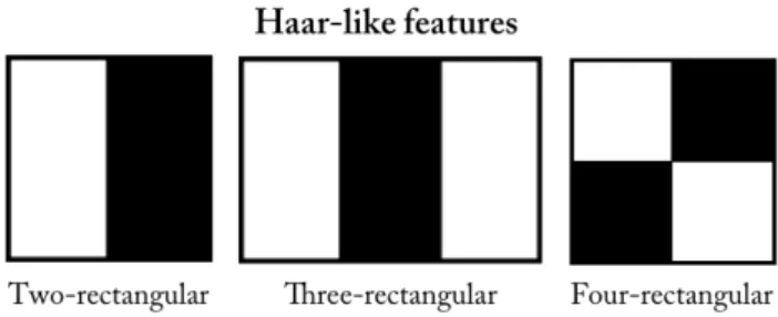
When designing a random forest classification algorithm, one has to decide what information or type of features the split function in the nodes of each tree should evaluate. In theory, any quantitative information in the image can be used as a feature. The choice of features will determine the accuracy and speed of the classification algorithm. Haar-like feature is a type of features first developed for image classification by Viola and Jones [25] in 2004 with its speed being the main advantage over other features. In a one-rectangular feature, the sum of the pixel intensities in a rectangle is calculated and used to classify regions in an image based on defined threshold values. The rectangle is randomly chosen and can have any position, size and shape within an image patch. In a two-rectangular Haar-like feature, the sum of the pixel intensities of two adjacent rectangular regions with the same shape and size are compared. The value of the difference is used to classify regions in an image. There are additional levels of Haar-like features where three or four adjacent rectangles pixel sum’s are compared, see figure 2.10. With higher level Haar-like features different textures, patterns and edges can be recognised in an image.[25]

Figure 2.10: Illustration of Haar-like features, with two- three-and four-rectangular features in the figure from the left.

To ensure that the tree chooses each new split that benefits the tree the most, it is important to measure and compare the information gain for every possible split. This can be done by comparing the ”purity” of the set before and after a split. It is desirable to have as high probability as possible for either true or false after a split.[24]

A way to quantify the certainty or ”purity” of a split is by calculating the entropy H of the set S in the node. The entropy H(S) depends on the probabil-ity of the positive and negative outcomes in the node, p(+)and p(−), as defined

in Equation 2.12. A completely pure node where there is a 100% probability of making a true classification has 0 entropy, while a completely uncertain 50/50 node has entropy 1.

H(S) = −p(+)log2p(+)− p(−)log2p(−) (2.12)

By comparing the difference in entropy before and after the split, it is pos-sible to calculate the information gain in each split as defined in Equation 2.13, where V is the random variable that the split is based on, S(−) and S(+) are

the sizes of the subsets with negative respective positive outcome and H(S(−))

and H(S(+)) are the entropies for the same subsets. For each new split, the

algorithm will choose the split with the largest information gain.

Gain(S, V ) = H(S) −S(−)

S H(S(−)) − S(+)

S H(S(+)) (2.13)

Since the features in each tree are randomly chosen, every tree will look different and give different probabilities of the output. When an unknown data is analysed, it will get a probability of being true or false from each tree. The forest gets its good accuracy from taking an average of the probabilities of all the trees. This means that even if one tree makes a ”bad” decision, the average from all the trees will be relatively accurate. This is a clear advantage of using the random forest along with it being relatively fast and not requiring a lot of storage.[24]

2.3.7

Deep Learning and Artifical Neural Networks

Inspired by the network of neurones in the human brain, artificial neural net-works have been developed in order to create better computer systems. The human brain can outdo a computer in many complex tasks thanks to its abil-ity to learn, classify and analyse things as well as store this information but yet have it easily accessible. In the brain, there is a vast network of neurones (1011_{), each one connected to about 10}4 _{other neurones, all working in parallel.}

Each neurone works as a processing unit, and it is believed that the memories are stored in the connections between the neurones. Comparing that to a com-puter, that normally has one processor and one memory, it is easy to see why we are looking at the brain to get inspiration on how to build better computer systems and algorithms.[23]

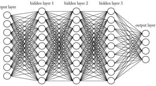
Figure 2.11: A simplified visualization of a deep neural network consisting of an input layer, three hidden layers and an output layer.

Deep learning is a machine learning algorithm using big artificial neural net-works (ANNs) consisting of multiple hidden processing layers. The term ’deep’ is often used when there are several layers in the neural network.[24] Compared to the random forest classifier that sets up trees with easily understandable rules on how to classify unknown data, the ANNs does not set up any rules that can be interpreted by the user. Based on training data, the hidden layers in the deep learning algorithm changes to improve the output, and the user does not have to program it and cannot see what is happening in the hidden layers.[1]

The basic structure of an ANN is the input layer, a number of hidden layers and the output layer. Each layer consists of a number of nodes, and each node is connected to all the nodes in the next layer as depicted in Figure 2.11. The nodes in the first layer receive the raw input data, for example, an image, text or sound, and extracts features from it. The first layer then transforms the data through non-linear modules into a slightly more abstract representation and send it to the next layer in the network that repeats this process. In this way, more and more abstract features are extracted for every layer deeper in the network, and the algorithm can learn very complex functions.[27]

The basic element in a neural network is a layer with nodes, also called the perceptron, a processing element which input may be raw input data or outputs from other perceptrons. Every input to a perceptron, xj∈ R, has a connection

weight tied to it, wj ∈ R, affecting the output, y. The output of a perceptron

can be written as

y = wTx + b (2.14)

in a layer and b is the bias.[23] A perceptron with only one node can be described as a linear function y = wx+b, and a sample data with a given input and output can be used to make a linear fit of the function. With more than one node in a perceptron, the definition in Equation 2.14 represents a hyperplane and a linear fit can instead be implemented with a set of samples with given inputs and outputs. In classification tasks, the hyperplane is used to divide the input data in a positive and a negative half-space based on the sign of the output

y(x) = (

1, if (wT_{x + b) > 0.}

0, otherwise. (2.15)

which gives a binary classification of the data in the perceptron. If it instead is desirable to get the probabilities of the of the classification, one can apply a non-linear sigmoid function to the output of the perceptron

y(x) = 1

1 + exp[−wT_{x + b]} (2.16)

A perceptron alone is sometimes called a single-layer perceptron (SLP). An ANN with multiple layers L of perceptrons is called a multi-layered perceptron (MLP). Compared to the SLP, the MLP consist of several non-linear layers. A non-linear element σ is therefore added to the definition in Equation 2.14 when applied in an ANN

y = σ(wTx + b) (2.17)

When data is sent through the multiple layers in an ANN in a feed-forward manner (one-directional), the signal is multiplied for each layer of perceptron, σ(wT_Lσ(w_L−1T ...) + w0).[28] In each hidden layer, a non-linear sigmoid element is

applied to the weights. The first layer receives the input xj, where j = 0, ..., d is

the number of inputs, and assign weights whj to them, where h = 1, ...H is the

nodes in the hidden layer. The sum of the weighted input data is transformed through a non-linear sigmoid function to zh, as defined in Equation 2.18. The

hidden layer assigns weights vi to the transformed data, where i = 1, ...K is the

number of output nodes. If there is more than one hidden layer in the ANN, the process is repeated for each layer. The output from the last layer yi is the

sum of the weighted transformed data from the last hidden layer defined in Equation 2.19. zh= sigmoid(wThx) = 1 1 + exp[−(Pd j=1whjxj+ b] , h = 1, ..., H (2.18) yi= vTi z (2.19)

In order to ensure that a given input x gives the correct output y, it is necessary to determine the weights by training the network on samples with given input and output. Two ways of doing this are through a pure end-to-end supervised training or by dividing the training in one unsupervised pre-training part and a supervised fine-tuning part. Two popular ways of doing end-to-end supervised training in medical imaging analysis are convolutional neural networks (CNNs) and recurrent neural networks (RNNs), while stacked auto-encoders (SAEs) and deep belief networks (DBNs) are popular for the latter two-step training method.[28] If the whole set of training data is available from start, all weights can be calculated offline, and when plugged into the perceptron, the output values will be calculated. Online training can instead take one training data at a time when available, making the network change over time when new training data is given.[23]

Convolutional Neural Networks

A fully connected MLP, as described in the section above, consists of a vast number of connections and parameters, making the training and testing of the algorithm time-consuming. CNNs were built to optimise the training process by utilising the fact that locally arranged pixels in images are correlated, represent-ing structures that can occur in different locations in the image, for example, edges and corners.[23, 28] A CNN is a network model with two main differences from other networks, namely weight sharing and feature pooling.[29] The weight sharing in a CNN is made possible by dividing the input image into subsets, usually referred to as receptive fields. In comparison to fully connected ANNs where each input node is connected to all the nodes in the next layer, the re-ceptive fields only have a small number of connections to the next layer. All receptive fields in a layer share the same weights, creating a feature map or filter for that convolutional layer. The reduced number of connections and weights to train, significantly increase the network’s efficiency.[29] Feature pooling is a non-linear operation that reduces the number of features in a feature map by taking only one value, for example, the maximum value, out of all feature values from each receptive field as output.[29] Repeating the convolutional layers with weight sharing followed by feature pooling enables the algorithm to combine previously learned features from different subsets into more complex features from the whole image.[23] This gives the CNN a hierarchical cone structure, where the features get fewer and more complex for every hidden layer until reaching the classes of the output layer.[23]

A typical CNN gives an output consisting of only a single class label to an input image, and because the output is a down-sampled version of the input image it cannot classify individual pixels.[30, 2] In many image segmentation tasks it is, however, desirable to classify each individual pixels in an image. There are many ways of achieving this found in the literature published the last few years, one is the fully convolutional network (FCN) proposed by Shelhamer et al.[30] An FCN gives an output image with the same spatial dimensions as the input image by adding additional layers to a CNN. The additional layers are referred to as deconvolutional layers and have an inverse architecture from

Author(s) Title Year published Paproki et al.[12] Automated segmentation and analysis of

normal and osteoarthritic knee menisci from magnetic resonance images - data from the Osteoarthritis Initiative

2014

Fripp et al.[31] Automated segmentation of the menisci from MR images

2009 Yin Y.[32] Multi-surface multi-object optimal image

segmentation: application in 3D knee joint imaged by MR

2010

Zhang et al.[33] The unified extreme learning machines and discriminative random fields for au-tomatic knee cartilage and meniscus seg-mentation from multi-contrast MR im-ages

2013

Sasaki et al.[34] Fuzzy rule based approach to segment the menisci region from MR images

1999 Swanson et al.[14] Semi-automated segmentation to assess

the lateral meniscus in normal and os-teoarthritic knees

2010

Tamez et al.[35] Unsupervised statistical segmentation of multispectral volumetric MR images

1999

Table 2.3: Previous work reviewed in this thesis.

the convolutional layers with the pooling operations replaced by upsampling operations. For the algorithm to be able to determine the spatial location of a feature after upsampling, it uses information from the contracting layers in the network.[30] Further modification of the FCN is proposed by Ronnerberger et al. [2], with the main difference being the introduction of a large number of feature channels in the upsampling part. This change makes the contract-ing and expandcontract-ing parts of the FCN almost identical, and the overall network architecture presume a u-shape, giving it its name UNet.

2.4

Review of Previous Work

There are many different image segmentation methods and algorithms applica-ble to medical imaging. However, few are applied to segmentation of the menisci in MR images. The following section will cover semi and fully automated meth-ods for segmentation of the menisci found in the literature. Seven articles are reviewed and the authors, titles and years published are found in Table 2.3.

Author(s) Magnetic Field Strength Sequence Resolution (mm) Slice thickness (mm) Paproki et al. 3 3D weDESS 0.37/0.37 0.7 Fripp et al. 3 FS SPGR 0.2343/0.2343 1.5

Yin Y. 3 3D weDESS 0.365/0.365 0.7

Zhang et al. 3 Multi-contrast 0.625/0.625 1.5 Sasaki et al. 1.5 T1 3D SPGR 0.625/0.625 1.5 Swanson et al. 3 T2 map 0.3125/0.3125 3

Tamez et al. n/a GRE n/a n/a

Table 2.4: Information about the image datasets used in the reviewed articles.

Author(s) Subjects Healthy/OA Sex Age 45 M 62.02 ± 10.89 Paproki et al. 88 Var. OA

43 F 60.42 ± 8.982

Fripp et al. 14 H n/a n/a

Yin Y. 9 Var. OA n/a n/a

8 M Zhang et al. 11 Unknown

3 F 24-41

Sasaki et al. 5 Mix n/a n/a

15 M 46-72 Swanson et al. 24 10 H / 14 OA

9 F 47-70

Tamez et al. 1 n/a n/a n/a

Table 2.5: Information about the subjects used in the reviewed articles.

2.4.1

Datasets

Paproki et al. [12] tested their segmentation method on 88 subjects, making it the study with the most number of subjects. The rest of the studies tested their algorithms on fewer subjects, ranging from one to 24 subjects. Fripp et al. [31] only tested their method on subjects with healthy menisci, while Sasaki et al.[34] and Swanson et al.[14] used a mix of healthy and degenerated menisci. Paproki et al.[12] and Yin Y.[32] tested their algorithms on subjects with varying grades of osteoarthritis. Tamez et al. [35] only tested their algorithm on one subject with unknown knee healthy condition using multispectral MR imaged fused from two different sequences. Zhang et al. [33] used multi-contrast MR images of the knee consisting of four sets of different sequences. The rest of the reviewed articles only used one MR sequence. A comparison and overview of the datasets and information about the subjects used in the reviewed articles can be found in Table 2.5 and 2.4.

2.4.2

Pre-processing

As a first step, Paproki et al.[12], Fripp et al.[31], Yin Y.[32], Zhang et al.[33], and Sasaki et al.[34] all normalised the intensity in the MR images used and ex-tracted the region of interest (ROI), i.e. the approximate menisci area. Paproki et al.[12] proposed to register an average knee MR image to the MR image to be segmented and extract the approximate menisci region based on the average knee menisci region. Fripp et al.[31] and Yin Y.[32] automatically segmented the bones and cartilage in the knee, while Zhang et al.[33] manually segmented the bones and Sasaki et al. segmented the femoral and tibial cartilage based on thresholding. The information gained from the bone and/or cartilage segmenta-tion allowed the process of extracting the approximate menisci region. Swanson et al.[14] had the most number of steps in the pre-processing part including selecting seed points in the menisci, defining the last slide to be segmented, re-moving regions not to be segmented and threshold determination based on the seed points. Tamez et al.[35] were the only reviewed study not requiring any pre-processing steps.

2.4.3

Segmentation methods

Paproki et al.[12] and Fripp et al [31] propose two different shape model (SM) based approaches for segmentation of the menisci. Paproki et al.[12] proposed a 3D active shape model (ASM) involving statistical shape models (SSMs) de-forming to likely menisci shapes based on the extracted approximate menisci region in the pre-processing stage and by comparing the grey level profiles with the average knee. Fripp et al.[31] positions average menisci shapes above the centroid of the axis between the lateral and medial tibial cartilage and deform the model to fit the image data by using 1D profiles at the normal to the surface. In the studies presented by Yin Y.[32] and Zhang et al. [33] machine learn-ing was used to train a classification algorithm uslearn-ing datasets of manually seg-mented menisci. Yin Y.[32] proposed to use a random forest classification al-gorithm while Zhang et al.[33] used a combination of the feedforward neural network extreme learning machine (ELM) classification algorithm that treats data as independent and identically distributed (i.i.d), in combination with a discriminative random field (DRF) algorithm, that takes spatial dependencies into consideration.

Sasaki et al. [34] proposed an approach to menisci segmentation based on a set of fuzzy if-then rules. The rules were derived from the knowledge that the menisci are anatomically located near the femoral and tibial cartilage surfaces and that the signal intensity of the menisci is coherent. Swanson et al.[14] seg-mented each slice through a simple thresholding operation based on the Gaus-sian model from the pre-processing stage followed by a morphological dilation operation to close gaps. Lastly, Tamez et al.[35] proposed a statistical region growing method where each voxel intensity is compared with its neighbours to determine if they are statistically similar and thus connect them to belong to the same region. This approach enables images with several regions to be

seg-Author(s) Segmentation method Automation level Segmentation time (min)

Paproki et al. 3D ASM Fully 27.2 ± 1.8

Fripp et al. SM fitting Fully n/a

Yin Y. Random forest Fully 20+1.5

Zhang et al. DRF + ELM Fully 1.348

Sasaki et al. Fuzzy logic Semi ca. 4

Swansen et al. Thresholding &

morphological operations Semi 2-4 Statistical

Tamez et al.

region growing Fully n/a

Table 2.6: Overview of segmentation methods for each reviewed article.

mented in the same time. A comparison of the different segmentation methods proposed and used in the reviewed articles, as well as the level of automation and segmentation time can be found in Table 2.6.

2.4.4

Post-processing

To compensate for possible over-segmentation, Zhang et al.[33] and Paproki et al.[12] both propose to estimate the menisci pixel intensity with a Gaussian distribution and exclude voxels with higher signal intensity than the mean value plus the standard deviation. To account for meniscal tears or signal changes within the menisci, they both make exceptions if the voxel with higher signal intensity lies within the internal parts of the segmented menisci. Swanson et al.[14] made a comparison of each slice with the previous one, and pixels not matching were tested based on their intensity value.

2.4.5

Validation and Results

Paproki et al.[12], Fripp et al.[31], Yin Y.[32], Zhang et al.[33] and Tamez et al.[35] evaluated their results by comparing it to manual segmentation done by either an expert segmenter or an expert radiologist. Swanson et al.[14] com-pared their results with manual segmentation done by operators of unknown experience level and Sasaki et al.[34] did not make any quantitative evaluation, but only a qualitative evaluation by a medical doctor. All studies, except Sasaki et al.[34], used the DSC to validate the results. In addition, Paproki et al.[12], Fripp et al.[31], Yin Y.[32], and Zhang et al.[33] validated their results using sensitivity and specificity. The validations of the segmentation results from pre-vious work are presented in Table 2.7 and 2.8. Zhang et al.[33] also tested and compared their suggested proposed approach with DRF, SVM, ELM and SVM combined with DRF.

Author(s) Meniscus DSC (µ ± σ) Comparison standard MM 0.783* Paproki et al. LM 0.839* Expert segmenter MM 0.77 ± 0.10 Fripp et al. LM 0.75 ± 0.10 Expert segmenter Yin Y. Both 0.80 ± 0.04 Expert segmenter Zhang et al. Both 0.82 ± 0.03 Expert radiologist No quantitative Sasaki et al. Both n/a

validation 0.80 ± 0.06† Swanson et al. LM 0.69 ± 0.12‡ Manual operator MM 0.5910* Tamez et al. LM 0.5373* Expert radiologist

Table 2.7: The DSC for the results reported in previous work and the meniscal side and comparison standard used. The DSC is given as the mean µ plus/minus the standard deviation σ. * Standard deviation not available. † Result for healthy menisci with no signs of OA or pain. ‡ Result for meniscus with different grade of OA.

Author(s) Meniscus Sensitivity (µ ± σ) Specificity (µ ± σ) MM 0.771* 0.9998* Paproki et al. LM 0.790* 0.9999* MM 0.72 ± 0.14 1.00 ± 0.00 Fripp et al. LM 0.72 ± 0.18 1.00 ± 0.00 Yin Y. Both 0.79 ± 0.06 1.00 ± 0.00

Zhang et al. Both 0.8395 ± 0.0575 0.9934 ± 0.0025

Sasaki et al. Both n/a n/a

Swanson et al. LM n/a n/a

MM Tamez et al.

LM n/a n/a

Table 2.8: Results from previous work. µ is the mean and σ is the standard deviation. * Standard deviation not available.

Chapter 3

Method and Material

This chapter covers the materials and methods used in order to achieve auto-mated segmentation of the menisci in the knee. Manual segmentation of the menisci was performed, described in section 3.2, in order to be used in the automatic segmentation methods as training data, as well as being used as the ground truth when evaluating the results. Two automatic segmentation algorithms, random forest based on Haar-like features and 2D UNet cascade segmentation, were implemented in this work as described in section 3.4 and 3.5 respectively. The MR image and subject data used in this work are described in section 3.1. Lastly, section 3.6 describes the evaluation metrics used to validate and compare the achieved results with the ground truth segmentation.

After initial training and testing of the Haar-like feature based random for-est and 2D UNet cascade segmentation, additional training and tfor-esting were conducted of the distal femur and articular cartilage using the 2D UNet cas-cade segmentation. The Haar-like feature based random forest segmentation was not trained or tested on the additional structures due to time limitations. The initial results from the 2D UNet cascade showed superior results compared to the random forest segmentation, and therefore this method was chosen for the training and testing of additional structures in the knee.

3.1

Image & Subject data

The image data used in this thesis were selected from Episurf Medical’s image database containing MR images of knees in the commonly used file format DI-COM. A vast majority of the knees in Episurf Medical’s database show different grades of joint degeneration. The subjects were randomly selected but had to fulfil an acceptable image quality and visualise the structure to segment without disturbing artefacts. To assure the image quality a visual check was performed. The experiments in this work were performed on 18 subjects for menisci

segmentation and 28 subjects for femur bone and cartilage segmentation. The menisci segmentation used two different MRI protocols, 12 scans were acquired with 3D T1 WE (or similar for other brands) and 6 scans with T2 de3D WE. The bone and cartilage segmentation used only a 3D T1 VIBE WE protocol (or similar for other brands). The images used were acquired with MRI scanners of different models from Siemens, General Electric (GE) and Philips. Information such as age, sex, scanner brand, model, magnetic field strength for each subject scanned for all subjects are found in Table A.1 and Table A.2 found in Appendix A.

In addition to the 3D sequence, a set of three standard 2D knee sequences from each subject were used in the experiments conducted in this thesis.1 The additional 2D sequences were Sag PD FS / Sag PD SPAIR, Cor PD FS and Tra PD FS.

3.2

Manual segmentation technique

Segmentations of the menisci, distal femur head and articular cartilage were re-quired in order to be used as training datasets for the automatic segmentation algorithms, as well as being used as ground truth when evaluating the segmen-tation results. The menisci from all 18 cases were manually segmented, while the distal femoral bone and articular cartilage had existing segmentations in Episurf Medical’s database. The manual segmentation was done using Mimics Medical v.18.02_{and 3-Matic Medical v.10.0}3 _{available from Materialise. In the}

manual segmentation process, both 2D and 3D sequences of the knee were used. The 3D image provided high resolution in all three planes, while the 2D images provided an excellent contrast of the menisci in each of the three planes, see Figure 3.1. The manual segmentation was performed in 2D PD FS sequences in three orthogonal planes; sagittal, coronal and axial/transverse. In each se-quence, a segmentation mask was created and a threshold value set to include the menisci voxels. To remove background voxels, the segmentation mask was cropped to a box including only the menisci. The opening morphological oper-ation was applied to the mask followed by a region growing operoper-ation as well as manual editing and cropping. 3D meshes were calculated from the masks in each sequence resulting in low-resolution 3D objects of the menisci from all three planes. The three 3D objects were merged to create a single model and smoothed to level out rugged surfaces. The solid 3D model was inserted in the high-resolution 3D sequence and any necessary final manual editing was done. The manual segmentations were reviewed by a radiologist. Figure 3.1 shows the final manual menisci segmentation as well as the femur bone and articular cartilage segmentations in the 3D sequence.

1_{Subject 78228559 did not have a Sag PD FS sequence, and subject EPB64 did not have}

a Tra PD FS sequence.

2_{http://www.materialise.com/en/medical/software/mimics (2016-10-01)} 3_{http://www.materialise.com/en/software/3-matic (2016-10-01)}

Figure 3.1: An example of 2D and 3D sequences from one subject, as well as the manual and existing segmentations of the menisci (red), femur bone (orange) and femur articular cartilage (white) used as training data, visualized in the 3D sequence.

3.3

Pre-processing

The range of pixel values in MR images vary and the histograms look different for each image. In order to aid training of the automatic algorithms and get more consistent results, outlying pixel values (top and low 5%) were trimmed and the rest normalised to grey values between 0 and 1000. The low 5% of the pixels were set to a grey level of 0, while to top 5% was set to a grey level of 1000. This is a common practice in segmentation tasks since it gives a more even pixel distribution which aids the algorithms to make correct classifications of pixels. In addition, the training and image data were converted to accepted file format for each software used in the following steps of the automated segmentation using the image processing software MeVisLab v.2.8.2 available to download for free from their website.4

3.4

Random Forest Segmentation

The random forest was trained and tested on 18 menisci in the software MIA lab5_{. The input data consisted of 3D image sets with corresponding manual}

menisci segmentations as the target object to segment and classify. The ran-dom forest consisted of 20 trees with 12 levels in each tree and was trained on randomly generated first and second order 3D Haar-like features in a randomly picked image patch of 32×32×32 voxels. In Table 3.1 is an overview of the parameters used in the random forest classifier implemented in the work in this thesis.

Parameter Value

Trees 20

Levels in each tree 12

Features 15 000

Patch size 32

Thresholds 10

Table 3.1: The parameters used in the imple-mentation of the random forest classifier.

4

http://www.mevislab.de/mevislab/ (2017-03-20)

3.5

Deep Learning

The deep learning algorithm was trained and tested on 18 pair of menisci and 28 distal femoral bones and articular cartilage. The menisci were trained in a single-class network. The femoral bone and articular cartilage were trained both separately in different networks and together on the same network, resulting in single- and multi-class outputs. In the single-class network, the Dice coefficient was used as loss function, optimising it for the output. The multi-class network as loss function, instead computes the categorical cross-entropy between the ground truth and the target.

The implemented algorithm is based on an existing algorithm, previously tested for segmentation of the liver and liver tumours. It is based on the fully convolutional network (FCN) with a 2D UNets architecture as reported by Ronnerberget et al.[2]. A few modifications have been made to the overall architecture, the main ones being the introduction of spatial dropout layers and the use of a cascade setup of UNets. The segmentation was implemented in Theano6 _{using the Keras framework}7_{, a library for high-level neural networks.}

Both Theano and Keras are written in Phyton and available to download for free from GitHub8

Big networks have some drawbacks, apart from usually being slow, overfit-ting can also be a problem if there is limited available training data. To address the problem of overfitting, spatial dropout layers were introduced in the imple-mented algorithm. These layers randomly drop units by temporarily removing them from the network during training, resulting in the training of ”thinned” networks. When performing testing of the network, the units are restored by averaging the predictions over all ”thinned” networks.[36] The spatial dropout rate used for the training implemented in this thesis was set to 0.40.

To improve the segmentation of 3D structures with the 2D UNets, the 3D volume was segmented in two orthogonal views by connecting two 2D UNets in a cascade setup. The algorithm setup starts by sending the input image to a 2D UNet for segmentation in the sagittal view. The output from the first UNet together with the input image are resliced and sent to the next UNet for segmentation in the coronal view.

The 2D UNet architecture implemented is illustrated in Figure 3.2 where the left side represents the contracting path, and the right side represents the expansive path. A total of 23 layers in the network was used in the implementa-tion in this work. The contracting path of the UNet uses a typical convoluimplementa-tional network architecture repeating a set of functions. The set starts with a 3x3 con-volution function, followed by a rectified linear unit (ReLU) activation function and lastly a 2x2 max pooling operation using 2 strides for downsampling and doubling the number of feature channels. The expansive path is a mirror of the contracting path, repeating up-sampling of feature maps, 2x2 ”up-convolution”

6

http://deeplearning.net/software/theano/index.html

7_{https://keras.io/}

8_{Theano: https://github.com/Theano/Theano (2017-05-21)}