How does inflation
expectation explain
the undershooting
of inflation target
in Japan?
BACHELOR
THESIS WITHIN: Economics NUMBER OF CREDITS: 15
PROGRAMME OF STUDY: International Economics
AUTHOR: Chung Shun MAN, Mark Peterson JÖNKÖPING June 2019
Time-series analysis within the
frame of hybrid Philips curve model
Acknowledgements
We would like to take this opportunity to show our immense gratitude for our thesis tutors, Emma Lappi and Marcel Garz. The time that you spent on preparing for the seminars, reading our thesis and listening to our feedback is invaluable to us. Your academic and emotional support indeed goes beyond your duty and helps us go through the difficult time during the process of the thesis. We truly believe your expertise and passion for teaching will continue to benefit the students in the university. Also, we would like to thank the students in our seminar group, including Ramil, Sakari, Katleho, Denusha, and Shirang. The seminars were stimulating with your active attendances. Your critiques helped us refine the thesis and make it possible.
Lastly, we would like to thank the most important people in our life. Our great friends like to share their knowledge and discuss rigorously on economics topics; our great family support us regardless of the results we will get; and our great teachers in Jönköping University strive to improve the quality of their courses and convey their knowledge to the new generation. You all deserve the best because you are the people in this world who are helpful, caring, and selfless.
Thank you all so much!
_______________________________ _______________________________ Chung Shun Man Mark Peterson
Jönköping International Business School May 2019
Bachelor Thesis in Economics
Title: How does inflation expectation explain the undershooting of inflation target? Authors: Chung Shun Man and Mark Peterson
Tutor: Emma Lappi and Marcel Garz Date: 2019-05-22
Key terms: Inflation target, Inflation expectation, rational expectation, adaptive expectation, Quantitative Easing (QE), Japan, Bank of Japan (BOJ)
Abstract
Inflation target was introduced in 2013 in Japan. The goal was to maintain price stability and sustainable inflation rate that is conducive to optimal consumption and investment decisions. However, Japanese inflation rate has been consistently below the target rate. We want to examine why the failure happens in such a big economy. This thesis focuses on inflation expectation as the main factor that leads to unanchored inflation. Inflation expectation can be distinguished into adaptive and rational expectation. To analyse inflation expectation, we regress inflation on four relevant variables: forecasted inflation, lagged inflation, economic slack and import inflation. Our goal is to identify the significance of forecasted inflation and lagged inflation, which are the main variables, to determine the characteristics of the two types of inflation expectation. This time-series analysis is on a monthly basis covering the period between 2013 and 2018. The results show that agents are near-rational rather than rational, meaning that they tend to overweigh the costs of inflation. Also, it is shown that they have minor but significant backward-looking tendency and believe that past inflation determines the current inflation. Hence, inflation expectation could give some useful insights into unanchored inflation.
Contents
1. Introduction ... 1
1.1. Background ... 2
1.2. Purpose ... 3
2. Theory and Literature Review ... 4
2.1. Demand side: Monetary policy and Inflation target ... 4
2.1.1. Quantitative easing ... 4
2.1.2. Taylor rule and inflation target ... 5
2.1.3. Big-bang and gradualist approach ... 6
2.2. Supply side: Formation of inflation expectations ... 7
2.2.1. Backward-looking expectations ... 7
2.2.2. Forward looking rational expectations ... 8
2.3. Phillips curve model ... 9
2.3.1 Nominal wage theory ... 9
2.3.2. Incorporation of inflation expectation theory ... 9
2.3.3. Hybrid Phillips curve model ... 10
3. Methodology ... 12
3.1. Dependent variable ... 12 3.2. Independent variables ... 12 3.2.1. Inflation expectation ... 12 3.2.2. Unemployment gap ... 13 3.2.3. Import inflation ... 13 3.3. Expected signs ... 13 3.4. Correlation analysis ... 14 3.5. Descriptive statistics ... 154. Empirical Model and Results ... 17
4.1. Econometric Model ... 17
4.2. Regression Analysis ... 17
4.2.1. Initial regression ... 18
4.2.2. Regression in corrected functional form ... 20
4.2.3. Interpretation ... 21 4.2.4. Robustness Check ... 22 4.3. Discussion ... 23
5. Conclusion ... 26
6. References ... 28
7. Appendix ... 32
1. Introduction
Inflation is a measure of a rate at which the average price of the consumption basket increases over a period of time. Inflation measures the increase in price, while deflation measures its decrease. Deflation leads to low average prices in the market. Cheaper products and services seem to be good at the first glance due to the higher purchasing power. However, persistent deflation can exert negative impacts on an economy, such as delaying purchase decision, preventing growth in nominal wage and depressing profitability of firms. One way to control deflationary pressure is inflation targeting - a central bank’s policy that aims at meeting and sustaining certain inflation level. Successful implementation of targeting can bring about the favorable price stability and predictability, which can stimulate current consumption and benefit country’s economy, as International Monetary Fund (IMF) (2018) says.
Japan introduced the inflation target in 2013, but it still fails to achieve it after 5 years. To understand the underlying reasons for unanchored inflation, we need to know the factors that determine inflation. There are major financial institutions such as IMF (2016) and Organisation for Economic Co-operation and Development (2011) that utilize an econometric model that includes the following elements: price of imports, inflation expectations and economic slack measured by rate of unemployment.
Among all the factors, inflation expectations could be the main contributor to the undershooting of inflation in Japan. Actual inflation is determined by consumers and firms, and so it could be strongly correlated with their inflation expectation. Kamada and Kakajima (2015) from Bank Of Japan (BOJ) say that if inflation expectations stick to the target rate, price stability can be maintained and contribute to sustainable development of the economy. There are different types of formation of the expectations. Rational expectation means that agents have sensible predictions that possibly push inflation towards the target, while adaptive expectation means that agents stick to the past inflation level. Sticky information and lack of rational expectation can lead to unanchored inflation and prevent the central bank from combating deflationary pressure. Thereby, in this paper, we will mainly discuss the role of inflation expectation and its deviation from the target. Based on the assumption about the importance of inflation expectation, our research question is: How does the inflation expectation explain the persistent undershooting of inflation target in Japan?
Investigation into the issue of deflation in Japan can contribute to our understanding of economic dynamics. From an economic point of view, in the long run low inflation decreases the incentive of labor to bargain for higher nominal wage, in turn leading to stagnant or decreasing real wage. But more importantly, we observe that the central bank shows its commitment by setting explicit target rate to eradicate the persistent deflation. The aggregate demand side in the economy seems to put pressure on the aggregate supply to raise inflation. But unanchored inflation still exists in Japan. The reasons we find are that the labor tend to be less rational at low inflation level, and the agents tend to have backward-looking inflation expectation, which is small but significant.
Other articles on inflation target usually focus on policies that aim at lowering the inflationary pressure to achieve the inflation target, in countries such as the United States (White, 2007), Euro zone and Swiss area (Reynard, 2007), and Spain (Caraballo & Dabús, 2013). Our article sheds light on its opposite: deflationary pressure. Persistent deflationary pressure can prevent growth in the nominal wage and raise concerns about the capability of monetary policies of central bank and behaviour of economic agents. Further, other articles discuss Japanese inflation and argue that factors such as the imperfect credibility of the monetary authorities and exchange rate shocks (Michelis & Iacoviello, 2016), and deflation biasedness of the monetary policy (Cargill & Guerrero, 2007) are its main drivers. Our article highlights the role of inflation expectation, the supply side that responds to the monetary policy and potentially leads to the undershooting of inflation target.
1.1. Background
If we zoom in and look at some of the key economic indicators for Japan, we can explore the overall dynamics of Japanese economy in recent years. With reference to the BOJ’s Outlook for Economic Activity and Prices (2019), Japanese exports, domestic investments, consumption and industrial production are following upward trend and unemployment is decreasing. Furthermore, the Bank of Japan indicates that the economy is operating with a positive output gap, which is likely to exert upward pressure on price level since the supply exceeds the capacity. However, the development of the Japanese inflation is modest, in relation to the indicators above.
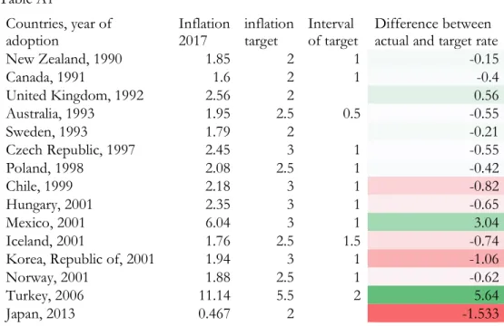
Table A1 in appendix shows the inflation targets of 15 OECD economies and their inflation rates in 2017. In 11 out of 15 OECD economies, the inflation rate fell below target. It seems
that falling short of the target is common. However, the inflation rate in Japan can be considered as an outlier compared to the other 10 economies, because the deviation of actual inflation rate (0.467%) from the target (2%) is the largest among the economies presented. Furthermore, the inflation target has been introduced since 2013 as a part of the policy package - called Abenomics (2012). The policy package was passed by Japanese Prime Minister Shinzo Abe and rested on three pillars: aggressive monetary policy; flexible fiscal policy, and a set of growth policies. The package aimed at stimulating inflation after two decades of economic stagnation through price stability that requires anchoring the inflation rate of 2%.
Figure A1 in appendix shows the development of inflation in Japan between 2013 and 2018. First, it shows a sign of rising inflation in 2014, which is the first year of fully enacting Abenomics. Nevertheless, later in the period the inflation had been falling short of the target and lingered around 0% in 2017. To explain why, Ito, Iwata, Mckenzie, and Urata (2018) argues that inflation expectations could be the main cause that drives down inflation. Hence, we want to examine whether inflation expectation plays an essential role in the unanchored inflation.
1.2. Purpose
The purpose of the thesis is to explain the factors that contribute to the deflation. We discuss the main economic theories to examine the connections between inflation and the main relevant variables. Literature reviews are used to figure out whether scholars support the validity of the economic theories. Based on them, we establish time-series econometric regression models to measure the impact of each explanatory variable on the dependent variable – inflation. To increase their robustness, formal significance tests are conducted to detect any violation of the OLS assumptions. The empirical finding discovers that agents are near-rational and tend to overweigh the costs of inflation. Also, they have slight but significant backward-looking expectation, meaning that past events could influence the current inflation. This research can improve our understanding about the associations among the key macro-economic variables, such as inflation expectation and labour union, on the supply side of the economy and monetary policy on the demand side.
2. Theory and Literature Review
The purpose of this chapter is to provide the theoretical background as well as literature reviews to the topics about monetary policy and inflation expectation. Then we will use the baseline hybrid Phillips curve model as a theoretical justification to support the regression model that will be tested in the empirical finding part.
2.1. Demand side: Monetary policy and Inflation target
Central banks introduce monetary policy by changing the money supply and interest rate and therefore play a crucial role in determining economic indicators such as inflation and GDP. Here we explain how monetary policy can be used to achieve an inflation target.
2.1.1. Quantitative easing
Quantitative easing (QE) is developed as a monetary policy in case of near-zero interest rate in the asset market. To understand the QE, we need to distinguish between short-term and long-term interest rates. A yield curve shows the time on the x-axis and interest rate on the y-axis and is upward sloping. According to Mundell-Fleming (1960) model, in case that short-term interest rate reaches nearly zero and the yield curve touches the origin, the economy is stuck in a liquidity trap. Orthodox monetary policy, which aims to buy the short-term bonds, is not effective in affecting output since short-term interest rate cannot be lower. Therefore, QE is developed to stimulate the output. QE can lower the cost of investment and stimulate the output. Meanwhile, buying long-term bonds can increase the money supply and maintain the same level of short-term interest rate. Bernanke, Reinhart, and Sack (2004) say that in a liquidity trap central banks can use QE to increase the money supply to lower the yields of non-money assets and the long-term interest rate. Thus, it is shown that QE takes advantage of both capital and asset market to push up output simultaneously. Also note that Kim, Hammoudeh, Eisa (2012), and Choudhry (2005) treat Japan as a flexible exchange rate regime and so monetary policy can be applied.
The quantitative and qualitative easing (QQE) in Japan gives a good example of QE. Shirai (2014) describes that QQE has two main features. First, it aims to increase the medium and long-term inflation expectations. According to real interest parity, nominal interest rate equals real interest rate plus inflation. QQE can be exploited to raise the inflation expectation while keeping the nominal interest rate constant. So real interest needs to go down and the
cost of investment can stay low. So it will lower the yield curve even if the short-term interest rate is about zero. Second, the central bank purchases Japanese Government Bonds (JGB) to expand the monetary base. It will extend the maturity of the JGB from 3 years to about 7 years by purchasing JGBs with maturities of up to 40 years. Thus it increases the outstanding amount of the Bank’s JGB holdings and the capacity to expand the monetary supply. Also, the JGB purchases can put downward pressure on the expected path of short-term interest rates. This can encourage more consumption and investments in other areas such as business and residential assets. Eventually, a low yield curve will encourage more borrowing and investment, in turn boosting output.
2.1.2. Taylor rule and inflation target
Monetary policy is important in determining output. Output and inflation are closely connected. Expansionary monetary policy can push up the aggregate demand, leading to higher output. From the supply side, actual output is above the potential level. This expansionary output gap implies that supply from firms and labor has exceeded their capacity. Inflation needs to grow to offset the higher total costs. Output drops to the level at which the supply meets the demand. The net impacts on inflation and output are positive in the initial period. Blanchard (1989) proves that demand shocks tend to move output and inflation in the same direction. Therefore, the model gives the implication that monetary policy can be used not only for output, but also for inflation.
To prove the link between monetary policy and inflation target, we can take a look at the Taylor rule (1993):
𝑖 = 𝛽 𝑖 + 𝛽 (𝜋 − 𝜋 ) + 𝛽 (𝑦 − 𝑦∗ )
𝑖 stands for interest rate. The rule specifies that monetary policy is set to eliminate the deviation of inflation rate from the target, referring to (𝜋 − 𝜋 ), and deviation of output from the potential output, representing (𝑦 − 𝑦∗ ). By doing so, the central bank can achieve the optimal level of inflation and output. Taylor rule has a close relationship with monetary policy since money supply has impact on the dependent variable 𝑖 .
Martin and Milas (2004) do a testing of an adjusted version of Taylor rule. The Taylor rule model is applied to the UK in two different regimes: the outer regime, where the inflation is
outside the target range, and the inner regime, where it is inside. The results find that 𝛽 , the coefficient for inflation difference, is significant higher in post-1992 in an outer regime. But when it comes to the UK in an inner regime, the two coefficients stay rather constant in the same period. The findings show that monetary policy aims at moving inflation back to the target rate rather than on output when inflation is outside the target range. On the other hand, the monetary policy seems unresponsive to minor changes in inflation when inflation stays around the inflation target. Therefore, monetary policy is a crucial instrument to grapple with severe deviation from the target rate, although it ignores small deviation.
2.1.3. Big-bang and gradualist approach
There are two main approaches to arrive at a new equilibrium inflation level: big-bang approach and gradualist approach. To start with, Deatripont and Roland (1995) say that the big-bang approach attempts to produce a desired rise in inflation in one giant step. The central bank needs to use expansionary monetary policy to raise the money growth substantially in the first period and slightly reduces it to meet the inflation target. This results in an enormous output gap and an overheated economy to push the actual inflation to reach the desired level. As a result, the inflation target is achieved in short time. However, we need to account for the cost of the big-bang approach. Overheating could inflate the risk of a bubble. It is the case when investors expect that firms could continue to produce with the output gap. The bubble bursts when investors are pessimistic about the future of the country and sell their assets in large number. Ito (2003) gives a vivid example of the Japanese economy during 1980s, when the economy was allowed to overheat and capital gains from securities and real-estate transactions were 40 per cent larger than GDP. After the implementation of 1988 Basel Capital Accord and Lending regulations in 1990, the bubble burst with a wealth decline equal to two years of GDP, as Bigsten (2005) proves. Therefore, a radical change in output suggested by the big-bang approach could be costly.
Instead, the policy makers often resort to the gradualist approach. Deatripont and Roland (1995) say that this approach attempts to accomplish a desired rise in inflation in a series of small steps. Money growth rises gradually and the gap between actual output and potential output is minimized. In comparison to the big-bang approach, the implementation of this approach is more difficult since it involves multiple periods and the central bank needs to keep track of the progress. But income gains that result from the rising money growth are
distributed over time. The approach also permits a more steady money growth to reduce volatility. Hence, the central bank will achieve the inflation target after multiple periods. 2.2. Supply side: Formation of inflation expectations
Individuals’ expectations play an important role in making inferences within the frame of economic analysis. There are two types of expectations: backward-looking and forward-looking. The former is a function of past variables, whereas the latter is a function of all relevant information available and is independent of shocks in the past. Price is a variable that can be determined by past events and information regarding the future. So in this section we discuss the price expectations.
2.2.1. Backward-looking expectations
Adaptive inflation expectation (AE) is a common type of backward-looking expectation. Nerlove (1958) states that individuals believe past events affect the current inflation, and deviation of expected prices from the actual prices should be corrected in each period. Therefore, the mechanism of adaptive expectation formation can be explained mathematically as:
𝑋∗− 𝑋 ∗= 𝑦[𝑋 − 𝑋 ∗], 0<y≤1 (1)
𝑋∗= 𝑦𝑋 + [1 − 𝑦]𝑋 ∗, (2)
Where
𝑋∗ is inflation expectation formed in period t for period t+1; 𝑋 ∗ is inflation expectation formed in period t-1;
𝑋 is the inflation observed in period t-1; 𝑦 is the coefficient of expectation.
Equation (1) means that the difference between current and lagged inflation expectation is a fraction of the difference between actual inflation in period t-1 and lagged inflation expectation. So agents revise their price forecast based on the past expectation mistakes they make. In addition, after rearrangement, we get the second equation (2). Nerlove (1958) claims that there are two main types of backward-looking inflation expectation. If the coefficient equals 1, then expected inflation in period t coincides with inflation observed in period t-1, in this case AE transforms into static expectation. In this case, the expectation is completely based on the past price level. It is also a case of sticky price, since price level is not predicted to change in the next period. On the other hand, if the coefficient equals 0, the expectation is said to be autonomous. In this case, the price expectation is fixed and is
independent from the past values. This type of backward-looking expectation implies that the formation of expectations is free from any shocks from the past.
DAD-SAS model can be used to describe the response of adaptive inflation expectation to actual inflation level. Suppose that an increase in the output pushes the inflation in the first period. In the second period, workers notice that they are working over their capacity and demand a higher wage consistent with a higher lagged inflation, and so they anticipate a rise in inflation. However, the inflation expectation is not high enough to close the output gap. The error in the prediction continues for many periods. The process slowly comes to a halt as output gap is getting smaller. In the long run, dynamic demand and supply meet with inflation level equal to money growth rate and output equal to potential level. Therefore, errors in predictions happen and last for a long period of time when inflation is based on backward-looking information1 . The dynamic properties of essential to DAD-SAS, ADAS
model were tested with a computer simulation in the work of Jose Gaspar (2018). Given the assumption that expectations are formed adaptively, the reasonableness of transitions from one equilibrium to another was proved correct.
2.2.2. Forward looking rational expectations
John Muth (1961) suggests that rational expectations are forward-looking and are based on predictions of future events based on all the available information and economic theory. Hence, individuals know how inflation reacts to various endogenous and exogenous factors.
We can also use the DAD-SAS model to analyze the features of rational expectation. Suppose again that in the first period expansionary policy pushes up the output and inflation. However, in the second period, the revision of expected inflation in rational expectation is different from the adaptive one. The agents know that to close the output gap, they need to anticipate even higher inflation. Thereby, the gap disappears due to their correct predictions. So the output restores to the potential level. In the following period, both inflation and output reach the long-run equilibrium and stay put. Accordingly, rational expectations minimize the prediction errors and help push the economy back to a stable equilibrium in relatively short period of time2 . As was mentioned in the work of Fiege and Pearce (1976),
1Gärtner, M. Macroeconomics, 5th edition (2016), p226-231 2Gärtner, M. Macroeconomics, 5th edition (2016),p232-235
rational expectations framework is consistent with the view of economists concerning the rationality of the behavior of economic agents.
2.3. Phillips curve model
We can use the Phillips curve model to show the interaction between inflation and inflation expectation and to provide theoretical framework for the regression model that will be run later.
2.3.1 Nominal wage theory
We learn that adaptive inflation expectation requires a long period of time for the economy to adjust to the equilibrium inflation, while rational inflation expectation can help restore to the equilibrium at a higher pace. Another crucial factor that determines inflation is the economic slack. Okun’s law (1962) states that the economic slack is measured by the gap between the actual and potential unemployment. In this section, we explain the relevancy of unemployment rate in the Phillips curve model.
Phillips curve model shows that when actual inflation gets lower than inflation expectation, the real wage rises. Therefore, in face of higher real wage, the cost of hiring labor rises, and firms need to reduce the labor force. Lipsey (1960) supports the negative correlation between the two variables. Therefore, in the labor demand side there is a negative correlation between inflation and unemployment gap in the short run. But in the long run, since unemployment is at the natural rate, price will adjust in proportion to money supply. Fuhrer (1995) argues that the correlation between inflation and unemployment is stable overtime. He adopts distributed lag model with lagged unemployment rate as independent variable and does a time series analysis. Fuhrer finds a net negative impact of the combined coefficients of lagged unemployment rate on the inflation. The result comes in favor of the nominal wage theory. 2.3.2. Incorporation of inflation expectation theory
Apart from the nominal wage theory, incomplete incorporation of inflation expectations can also explain why there is a trade-off between unemployment and inflation. Palley (2012) proposes the incomplete incorporation of inflation expectation theory.
Figure A2 in the appendix shows that the curve has an inflation threshold that separates a vertical Phillips curve with fully rational expectation above the threshold, and a “C” shape Phillips curve below it. The changes can be divided into 3 stages:
Starting from zero inflation, we assume that labor have near rational expectation and underestimate inflation. So inflation expectation is lower than actual inflation. It is because deflation is favorable. So any increase in inflation can expose their underestimation, lower their purchasing power and real wage, and increase unemployment. With a continuous growth in inflation and above minimum unemployment rate of inflation (MURI), wage erosion is getting worse and labor incorporate more inflation expectation, meaning that they will anticipate higher inflation rate and correct their underestimation. Lastly, if inflation rises above the threshold, unemployment is independent of inflation rate, since unemployment is only determined by other factors such as structural unemployment. Labor are rational and have full incorporation of inflation expectation, and inflation expectation and actual inflation should be closed.
This theory is important to explain why labor underestimate inflation. The degree of incorporation of inflation expectation, or the extent of the “C” shape, depends on labor militancy. A more bell-shaped curve implies weak labor militancy and their low bargaining power. Workers slowly incorporate inflation expectation and there is more room for reduction in unemployment rate. Therefore, monetary policy can be manipulated to increase inflation rate in the short run and reduce the unemployment rate. On the other hand, a more vertical curve means high labor militancy and labor can anticipate higher inflation and wage. Unemployment does not need to decline to accommodate a growth in inflation. Hence, weak labor militancy could lower their bargaining power and make inflation expectation sticky. To see whether underestimation of inflation exists, we can check the coefficients of inflation expectation. Brainard and Perry (2000) claim that the sum of coefficients of inflation expectation less than unity indicates underestimation. Also, they find that an increase in the coefficient of inflation expectation can be explained by higher labor militancy.
2.3.3. Hybrid Phillips curve model
Gali and Gertler (1999) introduce the baseline Phillips curve model with lagged inflation: Formula: 𝑝 = 𝜃 𝑝∗+ (1 − 𝜃) 𝑝 .
This is a baseline model excluding other relevant variables. We can interpret the formula this way: The fraction 𝜃 of firms that set their price at period t choose the optimum reset price 𝑝∗, while the remaining (1- 𝜃) of firms keep the prices unchanged at 𝑝 . Therefore, some firms are forward-looking, meaning that they use all the available information to set prices
optimally. On the other hand, the others stick to the backward-looking information. By studying the degree of 𝜃, we can measure the degree of price rigidity (i.e., 𝜃 = 0 represents complete price rigidity), and the frequency of price adjustment. Gali and Gertler (1999) apply the model in time series and the results show that 60 to 80 percent of firms exhibit forward looking price setting behavior. It means that agents believe in the information regarding the future. They conclude that inflation expectation has significant impact on current inflation. However, Gali and Gertler (1999) argue that the parameter for backward-looking behavior, although significant, is of limited quantitative importance. So exclusion of lagged inflation will not matter. Also, Swamy and Tavlas (2007) cast doubt on the importance of lagged inflation in the regression. They claim that an addition of lagged inflation to the Phillips curve model can result in misspecification and we cannot trust the estimates since the price does not have random walk. In addition, they claim that even if there is a significant correlation between price and lagged price, the true coefficient could be zero. Since both prices should be determined by the exogenous variables from the true model, such as inflation expectation and economic slack. Therefore, lagged inflation should be excluded from the model. In face of the issues of lagged inflation, remedies are needed to correct for the misspecification and measure the extent of backward-looking behavior. Chauvet, Hur, and Kim (2017) propose an adjusted version of the hybrid Phillips curve model. In this new model, we need to regress the first difference of inflation on the first difference of lagged inflation. Its coefficient is equal to (1-2θ/θ) where the parameter θ governs the relative importance of forward-looking inflation expectation with a mean of 0.5. It incorporates information regarding the inflation expectation behavior. If the parameter θ is more than 0.5, the coefficient of the first difference of lagged inflation is negative and inflation expectation is forward-looking, while the opposite is true if the parameter is less than 0.5. For example, the parameter θ was 0.61>0.5 in the sample from the US and the coefficient is negative. Thence, the inflation expectation in the US between 1960 and 2008 is forward-looking: change in the inflation rate is corrected in the next period and expectations on future economic activity play a more important role to determine inflation. In terms of the robustness, the tests show that the results are not sensitive to the model specification. Therefore, the hybrid Phillips curve model in its first difference form could have useful information regarding in inflation expectations.
3. Methodology
To illustrate relationship between inflation expectation and inflation, regression model is run. First, we explain the meanings and measurements of the variables included in our regression model.
3.1. Dependent variable
Inflation is the percentage change in the consumer price index for a specified period of time. In our case the inflation is the headline consumer price inflation that comes from Official Statistics of Japan. The data on consumer prices is available in the form of index. Laspeyres formula is taken to calculate the price index. Price index is calculated by dividing the multiple of nominal year price and base year quantity by the multiple of base year price and base year quantity. We will use the CPI statistics report covering 585 major items with 2015 as the base year. Then, the inflation is calculated as a percentage change in monthly CPI on a year-over-year basis.
3.2. Independent variables 3.2.1. Inflation expectation
Our main interest in the regression model is the two variables: forecasted inflation and lagged inflation. Lagged inflation is the rate in the previous month. It measures the persistence in inflation rate and gives us an estimate of the degree of adaptive inflation expectation. Contrary to lagged inflation, forecasted inflation considers all the possible and relevant events in the future and represents long-term inflation. Here we use inflation forecasts as estimates of expected inflation. Galianone, Issler and Matos (2017) support this estimation method. But finding the forecasts could be challenging because they are calculated by private companies and are usually hidden. Fortunately, there are three organizations, including Mizuho Research Institute, Mitsubishi UFJ Financial Group, and Mitsubishi UFJ Research and Consulting that provide free quarterly forecast of inflation in Japan. The estimates of inflation expectation differ among various organizations and we take the average of their estimates. Notice that the data for its estimate is on a quarterly basis. To conduct a monthly time-series analysis, we assume that monthly inflation forecast is the same every three months in a season. We might lose track of the monthly development of inflation. Nevertheless, converting quarterly into monthly data is our best solution due to data availability.
3.2.2. Unemployment gap
Unemployment gap is measured by the deviation of the actual unemployment rate from the natural unemployment rate, which is the Non-Accelerating Inflation Rate of Unemployment (NAIRU) that is consistent with an inflation rate that neither accelerates nor decelerates, as Hirose and Kamada claim (2002). The importance of unemployment gap is implied by the nominal wage theory and incorporation of expectation theory and it should be included in the model. Also, U* is the estimate of the time-invariant NAIRU in Japan in the sample period. The data comes from Official Statistics of Japan. Notice that economic slack is a controlled variable and the implication of the coefficient will not be discussed.
3.2.3. Import inflation
The import inflation is measured by the import price index, which is calculated by the same formula, as the CPI that Bank of Japan (2017) suggests. In our case, the indices include items that landed in Japan in a specific month. The indices also use year 2015 as the base year and adopt the fixed-base method. Additionally, it is worth mentioning that the prices of goods are measured in Japanese yen. This implies that changes in the index will reflect both the exchange rate movements and changes in price of the imported goods. Therefore, it is the variable that captures the external shocks abroad on domestic price. The data comes from BOJ database. It is also a controlled variable in our case.
3.3. Expected signs
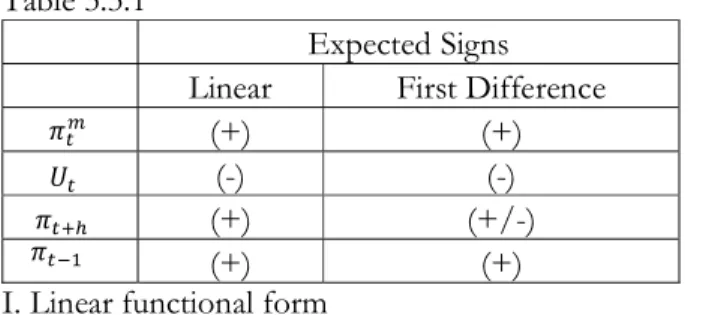
Table 3.3.1 below presents expected signs for the coefficients of the variables as well as the variables in the first difference form. The motivation for this will be given later.
Table 3.3.1
Expected Signs
Linear First Difference
(+) (+)
(-) (-)
(+) (+/-)
(+) (+)
I. Linear functional form
In line with the theory and literature about the Phillips curve equation in the linear form, we expect the coefficients of import price inflation, inflation expectation and lagged inflation variables to be positive; and the coefficient of unemployment rate to be negative.
𝜋 𝑈 𝜋 𝜋
II. First difference form
All coefficients except the one for lagged inflation are expected to have the same signs as those expected in the linear functional form. With reference to the adjusted version of the hybrid Phillips curve model, the coefficient of lagged first difference of inflation can be either negative or positive. A negative sign will hint that, within the given framework, forward-looking component of expectations is more important than backward-forward-looking, while a positive one will indicate the opposite.
3.4. Correlation analysis I. Linear functional form Table 3.4.1 𝜋 𝑈 𝜋∗ 𝜋 𝜋 𝜋 1 𝑈 0.0623 1 𝜋∗ – 0.2190 0.0031 1 𝜋 0.1618 0.0842 0.8059 1 𝜋 0.2186 0.1120 0.8209 0.9398 1
From Table 3.4.1 we observe that two independent variables: inflation expectation and lagged inflation are highly correlated. High linear correlation between two explanatory variables is a necessary, but not sufficient condition for imperfect multicollinearity. But we might start suspecting that multicollinearity is a potential problem. In Figure A3 in the appendix, we observe that inflation expectation and lagged inflation tend to move in somewhat the same direction over time. This might cause multicollinearity. There are several remedies to this issue, two of them are log and first difference transformation. Further, we observe that unemployment variable is positively correlated with the dependent variable, which runs counter to the Phillips curve theory. Positive correlation implies that the coefficient in front of unemployment variable has a positive sign as well.
Lastly, inflation expectation and lagged inflation have high correlation with inflation. That is to say that the coefficients of determination (R^2) are high as well. This, in turn implies that each of the two independent variables explains unusually much of the variation in the dependent variable.
II. First difference form Table 3.4.2 D(𝜋 ) D(𝑈 ) D(𝜋∗) D(𝜋 ) D(𝜋 ) D(𝜋 ) 1 D(𝑈 ) 0.0035 1 D(𝜋∗) – 0.1280 – 0.0697 1 D(𝜋 ) 0.0699 0.1175 0.0591 1 D(𝜋 ) 0.0315 – 0.0334 0.6251 0.2347 1 Table 3.4.2 depicts correlation matrix for the first difference form. One can observe that the coefficient for unemployment takes on the expected sign, both the correlation between inflation expectation and lagged inflation, and correlation between the two independent variables and the dependent variable becomes smaller. Also, since inflation expectation is adjusted on a quarterly basis, the first difference of inflation expectation in the second and third month in a season is zero. A reasonably high correlation between actual and expected inflation means that prices tend to be sticky on a monthly basis and are adjusted on a seasonal basis.
3.5. Descriptive statistics I. Linear functional form Table 3.5.1 Mean 1.65 % 3.22 % 0.85 % 0.87 % 0.87 % Max 18.64 % 4.30 % 2.80 % 3.74 % 3.74 % Min – 21.76% 2.30 % – 0.27 % – 0.93 % – 0.93 % St. Deviation 0.1211 0.0053 0.0087 0.0114 0.0113 Skewness – 0.5534 0.0533 1.2203 0.9681 0.9728
With reference to the data collected and table 3.5.1 we find out that maximum inflation (3, 74%) value is observed in May 2014. Monthly inflation values in year 2014 are significantly higher than that in other years (based on average annual inflation in 2014 which equals 2, 76%). This observation can be matched with the fact that Abenomics were enacted in 2014. The similar pattern is observed for inflation expectation variable: maximum value (2, 80%) is in 2014. One of potential explanations of this phenomena is that, with reference to the theory section and the regression model, workers and households understand the bank’s policy and revise their expectations in response to it because they observe higher inflation in
the previous period, in turn pushing up the actual inflation. However, the net effect on inflation should be evaluated when all other explanatory variables are also taken into account. This will be done in the forthcoming section. Skewness varies within -0, 55 and 1, 22 limit. The distribution for inflation expectation is strongly skewed to the right. Other variables show various degrees of positive and negative skewness. One of the suggested solutions is to log the variables, however, the time series contains both positive and negative values, and thereby the log transformation is not possible. As we said in the correlation analysis section, the linear form regression suffers from several flaws. The first difference form of the Phillips curve is expected to correct the misspecification errors of the linear regression.
II. First difference form Table 3.5.2 D(𝜋 ) D(𝑈 ) D(𝜋∗) D(𝜋 ) D(𝜋 ) Mean – 0.11 % – 0.03 % 0.01 % 0.02 % 0.01 % Max 7.20 % 0.30 % 2.00 % 1.76 % 1.76 % Min – 7.33 % – 0.30 % – 2.03 % – 1.55 % – 1.55 % St. Deviation 0.0306 0.0012 0.0038 0.0040 0.0040 Skewness -0.0572 0.2114 -0.3486 0.3913 0.3730
As one can notice in tables 3.4.2 and 3.5.2, the first difference corrects the discovered flaws of the linear form regression including the skewness of inflation expectation. Given the results above and the fact that log transformation is not possible, we adopt the first difference transformation to correct the potential misspecification of the model in the linear form.
4. Empirical Model and Results 4.1. Econometric Model
The monthly time-series analysis covers the period between 2013 and 2018 in Japan. This timeframe is chosen since our goal is to measure the formation of inflation expectation after the introduction of the inflation target. In this analysis, hybrid Phillips curve models in two different functional forms are tested.
First, we regress inflation rate on expected inflation rate, lagged inflation rate, unemployment, and import inflation to derive the hybrid Phillips curve model:
Model 1: 𝜋 = 𝛽 𝜋∗+ 𝛽 𝜋 + 𝛽 (𝑈 − 𝑈∗) + 𝛽 𝜋 + 𝜖
𝜋 = −𝛽 𝑈∗+ 𝛽 𝜋∗+ 𝛽 𝜋 + 𝛽 𝑈 + 𝛽 𝜋 + 𝜖
This model is based on the original Phillips curve model with lagged inflation to derive the hybrid Phillips curve model and import inflation to account for the external effects that affect domestic inflation. The intercept is a constant and is the negative multiple of potential unemployment and the coefficient of unemployment, as Ball and Gregory (2002) note in the case of time-invariant NAIRU. Since the model implies linear correlation between variables, we will apply OLS to get the estimates.
Second, the hybrid Phillips curve model in the first difference form is the equation at period t minus the same equation at period t-1. The model is as follows:
Model 2: ∆𝜋 = 𝛼 ∆𝜋∗+ 𝛼 ∆𝜋 + 𝛼 ∆𝑈 + 𝛼 ∆𝜋 + 𝜖
This hybrid Phillips curve model in the first difference has different coefficients, because this model explains that one unit increase in changes of the independent variable leads to 𝛼 unit increase/decrease in changes of the dependent variable. So the interpretation is also different. Also, since intercept is a constant, the first difference of the intercept is zero.
4.2. Regression Analysis
The following tables show the results obtained from the two regression models. We can check whether the coefficients and signs make economic sense. Also, the models are checked for possible misspecification to see whether we can trust the estimates. Autocorrelation is a potential problem since a lagged dependent variable is included.
4.2.1. Initial regression
First, we run the hybrid Phillips curve model with variables in the absolute values and see whether we can draw inference from the results. Note that throughout the tests we use the significance level of 5%
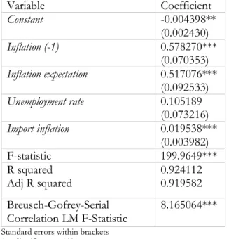
Table 4.2.1 Regression results: Dependent variable: inflation
Variable Coefficient Constant -0.004398** (0.002430) Inflation (-1) 0.578270*** (0.070353) Inflation expectation 0.517076*** (0.092533) Unemployment rate 0.105189 (0.073216) Import inflation 0.019538*** (0.003982) F-statistic 199.9649*** R squared Adj R squared 0.924112 0.919582 Breusch-Gofrey-Serial Correlation LM F-Statistic 8.165064***
Standard errors within brackets * = Significant at 10% ** = Significant at 5% *** = Significant at 1% N=72
Source: Portal site of Official Statistics of Japan, BOJ Time-series Data search, Mizuho Research Institute, Mitsubishi UFJ Research and Consulting, Mitsubishi UFJ Financial Group
The table above shows that all variables have the expected positive signs, except for unemployment rate with an unexpected positive sign. Also, R squared is 92.4112%, meaning that the four variables in the model explain 92.4% of the variation of inflation. Inflation measures the increases in price levels on aggregate, and so it is affected by many variables. Hence, the R squared is unexpectedly high and we should be cautious of the interpretation of the coefficients.
The unusually high R squared and high significance of coefficient of lagged inflation may cast doubt on the model. Hence, we need to check any misspecification and determine whether this hybrid Phillips curve model is spurious. First, a Breusch-Godfrey test can be used to detect autocorrelation.
𝐻 : 𝑛𝑜 𝑎𝑢𝑡𝑜𝑐𝑜𝑟𝑟𝑒𝑙𝑎𝑡𝑖𝑜𝑛 𝐻 : 𝑎𝑢𝑡𝑜𝑐𝑜𝑟𝑟𝑒𝑙𝑎𝑡𝑖𝑜𝑛
Table 4.2.1 above shows the result of the statistics for autocorrelation. Since the F-statistics is 8.165 and the p-value is below 0.05, we can reject the null hypothesis and say that there is autocorrelation in the linear hybrid Phillips curve model. It means that the residual at period t is correlated to residual in period t-1. The consequence of
autocorrelation is the underestimation of the variances of the regressors, in turn increasing the test-statistics. It inflates the risk of rejecting null hypotheses that the regressors are insignificant and the risk of committing type 1 error.
Linde (2005) also notes that New-Keynesian hybrid Phillips curve using single equation methods can give unreliable estimates of the parameters. If inflation is intrinsically
persistent as the other explanatory variables, it can give unbiased results. But if it is not, the significance of lagged inflation could originate from inertia in the aggregate demand and policy rule. So the model could support the backward-looking Phillips curve, even though the Phillips curve is forward-looking. And remedies are needed to correct it. Therefore, in our case the highly significant coefficient of lagged inflation could result from stickiness of the economic conditions. We cannot conclude that the agents in Japan are backward-looking.
Our robustness test supports the view that the first hybrid Phillips curve model is spurious, and the estimates should not be trusted. However, we need to measure backward-looking inflation expectation and study the behavior of agents who form the inflation expectation. Therefore, an alternative model is proposed to fix the misspecification.
4.2.2. Regression in corrected functional form
The variables of hybrid Phillips curve model are relevant according to economic theory. To keep the originality, we regress the first difference of the dependent on the first difference of independent variables to obtain the results below.
Table 4.2.2 Regression results Dependent variable: D (inflation)
Variable Coefficient Constant -0.0000336 (0.000372) D (Inflation (-1)) 0.195578** (0.094846) D (Inflation expectation) 0.654470*** (0.097769) D (Unemployment rate) -0.041616 (0.303639) D (Import inflation) 0.012706 (0.012070) F-statistic 13.12360*** R squared Adj R squared 0.439581 0.405617
Standard errors within brackets * = Significant at 10% ** = Significant at 5% *** = Significant at 1% N=71
Source: Portal site of Official Statistics of Japan, BOJ Time-series Data search, Mizuho Research Institute, Mitsubishi UFJ Research and Consulting, Mitsubishi UFJ Financial Group
The results from table 4.2.2 show that inflation expectation is significant at 1%, and lagged inflation is significant at 5%. The unemployment rate and import inflation have the expected signs, despite their insignificance. The constant is nearly zero since the constant of the regression at period t and that at period t-1 are the same. R-squared turns out to be only 43.96%. But notice that the first difference can remove any possible linear trend in the variables. So it may not give an interpretation of the variation that the model explains. We can use the F-test to see the overall significance of the model.
𝐻 : 𝛽 = 𝛽 = 𝛽 = 𝛽 = 0
𝐻 : 𝑎𝑡 𝑙𝑒𝑎𝑠𝑡 𝑜𝑛𝑒 𝑜𝑓 𝑡ℎ𝑒 𝛽 ( , , , ) 𝑖𝑠 𝑠𝑖𝑔𝑛𝑖𝑓𝑖𝑐𝑎𝑛𝑡𝑙𝑦 𝑑𝑖𝑓𝑓𝑒𝑟𝑒𝑛𝑡 𝑓𝑟𝑜𝑚 𝑧𝑒𝑟𝑜
Table 4.2.2 shows that the F-statistic is 13.12 and is significant at 1%. Therefore, we reject the null hypothesis and we can say that the model overall can be used to estimate inflation.
4.2.3. Interpretation
Both inflation expectation and lagged inflation are significant. The first most significant variable is inflation expectation. A unit change in the first difference of the inflation expectation is correlated with 0.6545 unit change in the first difference of actual inflation. It implies that agents could predict a decrease of one unit in inflation in the future, but it only results in a decline of 0.65 unit. So it indicates that the agents tend to underestimate inflation. The result seems to be consistent with Palley’s argument that low inflation is associated with underestimation of inflation. The agents that predict inflation tend to incorporate less inflation expectation at a low rate due to their preference for higher purchasing power. Figure A3 in the appendixshows that before year 2014 the Japanese agents do underestimate inflation. And when inflation soars, labor realize that they are losing purchasing power and command a higher wage, pushing up the inflation
expectation. So the expected inflation does rise and stays on a higher level between year 2014 and 2015. But since inflation returns to around 0 percent, its expected rate drops and is unresponsive to rises in actual inflation and lingers at 0.8 percent. It signifies near-rational expectation since some agents are near-rational but tend to ignore low inflation rates. The second most significant variable is lagged inflation. In Table 4.2.2, the result means that a unit change in the first difference of lagged inflation leads to a positive 0.1956 change in the first difference of inflation. To illustrate, if the inflation decrease in the previous period is 1 percentage point, inflation in the current period will go in the same direction to drop by 0.2 percentage point. It means that the declining trend is persistent and is difficult to reverse. Also, Chauvet, Hur, and Kim (2017) argue that a positive sign of the lagged coefficient means a backward-looking inflation expectation. Although the coefficient of 0.2 is small and only significant at 5%, it could give some interpretation about the expectation formation behavior. Past inflation is likely to impact future inflation. The impact of economic shocks will gradually disappear after several periods of time. It therefore shows signs of adaptive inflation expectation.
4.2.4. Robustness Check
There is a lagged dependent variable in the new model. To determine the robustness of this model, we can use the Breusch-Godfrey test to detect autocorrelation. The null hypothesis is the same as in the initial regression part. The results in table A2 in the appendix show that the p-values of the two test-statistics are far above 5%, indicating that we do not reject the null hypothesis and thus say that there is no autocorrelation. Second, Breusch- Pagan-Godfrey test is used to detect heteroscedasticity. The null hypothesis is that there is no heteroscedasticity. The results in Table A2 show that the p-values of both statistics are above 5%, meaning that the residuals do not exhibit any heteroscedastic pattern. Therefore, we do not reject the null hypothesis and thus say that there is no heteroscedasticity. Third, variance inflation factor is adopted to detect any multicollinearity. Gujarati (1988) says that a VIF=0 means that there is no multicollinearity. And VIF>10 implies serious multicollinearity. Table A3 shows that both uncentered and centered VIF are nearly 1 for all the variables. Thus, we can say that there is no multicollinearity. Therefore, the variances of the estimates are good approximation of the true variances. And we can trust the t-statistics and say that inflation expectation and lagged inflation in their first difference form are significant.
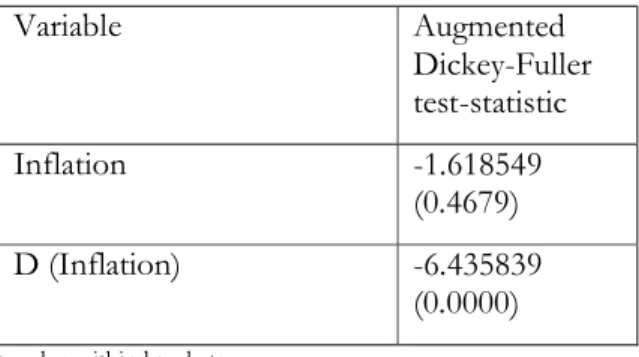
In fact, a lagged dependent variable no longer causes autocorrelation since the first difference turns inflation from nonstationary to stationary time-series by removing linear trend. We use the Dicker-Fuller (DF) test to detect a unit root of the time-series. The null hypothesis of the test is that the variable has a unit root. First, the results in Table A4 show that the p-value of the DF statistic for inflation is 0.4679, far above 0.05. Therefore, we do not reject the null hypothesis that inflation has a unit root. It means that inflation has a stochastic process that shows tendency to move upward and downward without returning to the mean.
Second, the results show that the p-value of the DF statistic for the first difference of inflation is 0.0000 below 0.05. Hence, we reject the null hypothesis that inflation has a unit root. So we can say that the first difference of inflation is a stationary process. The time-series has constant mean and variance. It also tends to revert to the mean and is thereby predictable.
Besides, we can observe the pattern of inflation in the first difference form. Figure A3 shows the pattern and indicates that there is one spike in April 2014 and is the other one in April 2015. They represent the period of the explicit and strong announcement of the target rate and rise in money growth. One solution to capture the changes is to insert two dummy variables into the regression. Table A5 shows the robustness test that controls the two periods. The results show that the dummy variables are highly significant at 1%. However, expected inflation becomes insignificant. The results imply that without the radical movements in inflation, expected inflation does not explain variation in inflation in their first difference form. This gives us a second interpretation of the variable of the expected inflation. With announcement of inflation target, firms and households anticipate the impact of monetary policy such as QQE and revise their expectation. So it gives them power to forecast inflation. On the other hand, without that clear information, expected inflation seems to perform poorly to anticipate inflation. A possible reason is that there are other explanatory variables become more significant to affect inflation and are not captured by the expectation. Therefore, expected inflation seems to be sensitive to announcement of monetary policy.
4.3. Discussion
The section focuses on the underlying meanings of the coefficients of the regression results and policy evaluation. It will begin with the bargaining power of the labor union to explain why near-rational expectation exists in Japan. And it will turn to analyze the positive and negative sides of the Qualitative and Quantitative Easing as the monetary policy. Then it will end with the implication of our regression results.
First, the incorporation of inflation expectation theory predicts that the responsiveness of inflation expectation has to do with labor militancy. Palley (2012) claims that low labor militancy means that labor union are weak and have low bargaining power to get higher wages, and it could explain why expected inflation is low. We can discuss the power of the labor union in Japan.
It is possible that the labor union is not inclusive enough and lacks bargaining power. The Japanese trade union seems to be biased towards regular employment in Japan. Rosetti (2018) argues that trade union in Japan represent interest exclusively of regular workers instead of their non-regular counterparts and women. Non-regular workers are among in
basic jobs such as commerce and general services. Their interest such as minimum wage should be distinguished from the interest of the regular workers, who in general have more stable and higher income. Hence, non-regular workers are usually ignored in the trade unions bargaining process, and so their wage is determined by the market and any legal requirement. For example, in Rengo (2017), the biggest trade-union in Japan, there are only 15.8% of non-regular workers and 36.2% of female in the total membership, compared to 37.5% of non-regular and 44.2% of female employment in the Japanese economy in 2016 and 2017. Lack of inclusiveness could lower their bargaining power for higher wage, in turn making inflation expectation stickier at a low level.
Beside the inclusion of labor, statistics from OECD (2019) shows that between 2007 and 2017, the growth of annual wage measured in current prices in domestic currency is about -1.15% in Japan, compared to 19.55% in the UK, and 22.36% in the US. It is possible that the Japanese labor union has less bargaining power than other developed countries and therefore wage becomes sticky.
Second, the Japanese monetary policy may also result in the failure to achieve the inflation target. Monetary policy can be implemented through two ways: interest rate and money supply. Bank of Japan (BOJ) implements the Quantitative and Qualitative Easing (QQE) so as to lower the yield curve and the short- and long-term interest rate. (Bank of Japan, 2016) However, Greenwood (2017) points out its downsides and argues that they ignore the money supply side of the monetary policy, which is related to broad monetary base, or M2. BOJ attempts to increase the money supply by buying securities from bank sectors instead of the nonbank ones. The commercial banks are usually risk-averse and keep the same level of lending. They are contrary to the private sectors, which could take the deposit and have higher liquidity to make investments. Therefore, the QQE policy will have limited impact on M2. It may explain why increase in demand is insufficient to cause a shift in inflation after 2015.
Even if QQE increases the money supply, successfully achieving the target looks challenging to Japan. It is because BOJ still needs to find the right approach to accomplish the target. Inflation rises substantially from 0.3% in 2013 to 2.8% in 2014. It seems true that BOJ follows a big-bang approach that dramatically pushes up the money growth rate. But inflation undershoots and returns to a low level later on. The reason could be the concern for
overheating economy. Constantly high level of output and inflation could cause investors to overestimate the returns on their investments. Instead, after 2014 Japan seems to follow the gradualist approach to hit the target. It requires a reasonably long period of time to ensure stability. Fujiki and Tomura (2017) argue QQE needs to keep ongoing at least until 2017, longer than 2015 that BOJ initially planned. They propose a careful exit strategy that can be used to prevent huge accounting losses at the end of QQE due to the decline in the market price of its long-term bond holdings. And a loss-sharing scheme with the government needs to be developed to relieve the burden of the BOJ. It suggests that QQE needs to last for certain period of time.
However, for the upsides of QQE, it seems to have anchored inflation expectation. Rukuda and Soma (2019) find a structural change in inflation expectation after the implementation of QQE in 2013. It is because BOJ has an explicit target to fight deflationary pressure. But the expectation is not high enough to reach a sustainable level of 2%. So they support the view that 2% target would not be feasible in the short run. Hence, gradualist approach seems appropriate for the inflation target to be achieved.
Last, a significant estimate might have different implications. Ones need to be aware that a significant result of expected inflation can imply correlation, rather than causality. The reason for the rise in expected inflation could be the explicit statement of the target rate (2013), while the rise in inflation could originate from expansion of the purchases of long-term bonds. Expected inflation and actual inflation could share similar trend, but they might not cause each other to move. Our argument in the interpretation section is that expected inflation could change that costs of input, such as labor wage, to influence actual inflation. Our simple regression model can show support for our argument. But more evidence is needed to see how one causes the other.
5. Conclusion
From the results of the regression model, we can identify the characteristics of the formation of inflation expectation in Japan. The conclusion will start from the demand side that the government and central bank can influence, to the supply side that firms and labor adjust in response to the demand shocks.
Monetary policy is an instrument to help inflation rate restore to the target rate. Taylor rule proves that nominal interest rate is based on the target interest rate, deviation of actual inflation from the target rate, and deviation of actual output from the potential output. By studying the data, Japan seems to be in the outer regime, where the inflation rate drifts away from the target rate. It is because a successful level of inflation should drift around the 2% target rate. Therefore, it seems reasonable that the Japanese monetary policy in recent years aims at inflation instead of output.
Quantitative and Qualitative Easing (QQE) is implemented to increase the monetary base and further lower the long-term interest rate. It will also extend the maturity of the JGBs to increase the number of bonds outstanding and boost the capability to expand money supply. Greenwood (2017) argues that it has ambiguous impacts on broad money supply. But Rukuda and Soma (2019) claim that QQE changes inflation expectation by explicitly stating the target. After all, they all agree that a 2% target would not be feasible in the short run. So the gradualist approach seems optimal to allow a stable path to hit the inflation target. Our main findings are that rational expectation and adaptive expectation can both be used to explain the formation of inflation expectation in Japan. When it comes to rational expectation, the agents seem to be near-rational rather than rational, since they ignore the benefits of inflation. It is proved by their underestimation of inflation rate. The two main reasons are that low inflation rate enhances the purchasing power of the labor in the short run, and that lack of labor militancy reduces the bargaining power to bid for even higher wage. Nominal wage theory focuses on the relevancy of unemployment while incorporation of inflation expectation theory emphasizes inflation expectation. In our analysis, the incorporation theory seems to better explain the causes of unanchored inflation.
In terms of adaptive expectation, the agents seem to be backward-looking. The expectation is subject to the past shocks, whose impacts will gradually fade away. Therefore, AE seems to be static rather than autonomous. But notice that the extent of backward-looking behavior is small despite its significance and our analysis is done on a monthly basis. Hence, more proof is needed to determine whether the agents stick to the past information.
There are some recommendations for Japan to raise expected inflation. Christiano, Eichenbaum and Rebelo (2011) suggest that increase in government spending under zero-nominal interest rate can push up output and inflation, in turn lowering the real interest rate. Then it will encourage more private investment and raise expected inflation. However, the effect depends critically on how agents value the costs of anticipated inflation. Also, one article even suggests a 3% inflation target rate (Moss, 2019). But radical measures should be taken with caution as the big-bang approach suggests that a large and temporary increase in output could overheat the economy and mislead investors.
We conclude by highlighting directions for future research. First, our analysis assumes that inflation expectation is measured based on the forecasts from large organizations. Future research can consider household surveys that reveal their anticipation regarding the future prices and determine whether inflation is getting more favorable. Second, our analysis focuses on Quantitative Easing as the key driver in the demand side. But the credibility of the central banks should also be considered. A highly credible central bank can convince the agents that high inflation will lead to economic boom and change their expectation, as Michelis and Iacoviello (2016) argue. Third, our results suggest that lack of bargaining power of the labor union over wage could result in sticky low inflation. But more evidence is needed to see how expected inflation is affects the actual one. Fourth, the time frame of the regression can be expanded to cover the period before 2013 by introducing dummy variables. It can reveal possible structural changes and deepen the analysis.
This paper aims at studying the impact of inflation expectation on actual inflation in Japan when the inflation target is in effect. But the behavior of inflation expectation could differ depending on the time span subject to the analysis and be modelled in other ways. Moreover, there could be other significant variables that are correlated with inflation. Further research can be done on the importance of inflation expectation and other relevant variables that lead to unanchored inflation in Japan and other countries.
6. References
Asao, Y. (2010). Overview of Non-regular Employment in Japan. The Japan Institute for Labour Policy and Training.
Ball, L., & Gregory Mankiw, N. (2002). The NAIRU in Theory and Practice. Journal of Economic Perspectives, Volume 16, Number 4, 122.
Bank of Japan . (2017). Outline of the Corporate Goods Price Index (CGPI, 2015 base). Bank of Japan .
Bank of Japan. (2013, January 22). Joint Statement of the Government and the Bank of Japan on Overcoming Deflation and Achieving Sustainable Economic Growth. Retrieved from https://www.boj.or.jp/en/mopo/outline/qqe.htm/
Bank of Japan. (2016). Developments in Inflation Expectations over the Three Years since the Introduction of Quantitative and Qualitative Monetary Easing (QQE). Bank of Japan. Bank of Japan. (2016, September 21). New Framework for Strengthening Monetary Easing:
"Quantitative and Qualitative Monetary Easing with Yield Curve Control". p. 1. Bank of Japan. (2019). Outlook for Economic Activity and Prices. Bank of Japan.
Beidas-Strom, S., Choi, S., Furceri, D., Gruss, B., Celik, S., Koczan, Z., . . . Lian, W. (2016). Global disinflation in an era of constrained monetary policy. World Economic Outlook, p. 130.
Bernanke, B. S., Reinhart, V. R., & Sack, B. P. (2004). Monetary Policy Alternatives at the Zero Bound: An Empirical Assessment. Brookings Papers on Economic Activity, 1-100. Bigsten, A. (2005). Can Japan Make a Comeback? World Economy, 596-597.
Blanchard, O. (1989). A traditional interpretation of macroeconomic fluctuations. American economic review, 1146-1164.
Brainard, W. C., & Perry, G. L. (2000). Editors' Summary. Brookings Papers on Economic Activity. Caraballo, M., & Dabús, C. (2013). PRICE DISPERSION AND OPTIMAL INFLATION:
THE SPANISH CASE. Journal of Applied Economics, 49-70.
Cargill, T. F., & Guerrero, F. (2007). Japan's Deflation: A Time‐Inconsistent Policy in Need of an Inflation Target. International Finance, 115-130.
Chauvet, M., Hur, J., & Kim, I. (2017). Assessment of hybrid Phillips Curve specifications. Economics Letters.
Choudhry, T. (2005). Exchange rate volatility and the United States exports: evidence from Canada and Japan. Journal of The Japanese and International Economies, 51-71.
Christiano, L., Eichenbaum, M., & Rebelo, S. (2011). When is the Government Spending Multiplier Large? Journal of Political Economy, 78-121.
Dewatripont, M., & Roland, G. (1995). The design of reform packages under uncertainty. American economic review, 1207-1223.
Feige, E., & Pearce, D. (1976). Economically Rational Expectations: Are Innovations in the Rate of Inflation Independentof Innovations in Measures of Monetary and Fiscal Policy? Journal of Political Economy, 499-522.
Fuhrer, J. C. (1995). The Phillips Curve Is Alive and Well. New England Economic Review. Fujiki, H., & Tomura, H. (2017). Fiscal costtoexitquantitativeeasing:thecaseofJapan. Japan and
the World Economy 42, 1-11.
Fukuda, S. I., & Soma, N. (2019). Inflation target and anchor of inflation forecasts in Japan. Journal of the Japanese and International Economies.
Gaglianone, W., Issler, J., & Matos, S. (2017). Applying a microfounded-forecasting approach to predict Brazilian inflation. Empirical Economics, 137-163.
Galí, J., & Gertler, M. (1999). Inflation dynamics: A structural econometric analysis. Journal of Monetary Economics.
Gaspar, J. (2018). Bridging the Gap between Economic Modelling and Simulation: A Simple Dynamic Aggregate Demand-Aggregate Supply Model with Matlab. Journal of Applied Mathematics.
Government of Japan. (2012). Abenomics. Retrieved from https://www.japan.go.jp/abenomics/index.html?fbclid=IwAR1I5ggJYD6LXCcd MuCHS6IxYDCjNTd_KRP-yMOAcLshdjb9dyuOL4XqAE4
Greenwood, J. (2017). The Japanese Experience with QE AND QQE. Cato Journal, 17-38. Gujarati, D. N. (1988). Basic Econometric. New York: John Wiley.
Hirose, Y., & Kamada, K. (2002). Time-Varying NAIRU and. Working Paper Series, 2, 10-11, 26.
Hogen, Y., & Okuma, R. (2018). The Anchoring of Inflation Expectations in Japan: A Learning-Approach Perspective. Bank of Japan Working Paper Series, 2.
IMF. (2016). Global Disinflation in an Era of Constrained Monetary Policy. World Economic Outlook, 130, 137, 147-149.
IMF. (2018, 12 18). Inflation: Prices on the Rise. Retrieved from International Monetary Fund: https://www.imf.org/external/pubs/ft/fandd/basics/inflat.htm?fbclid=IwAR3oD ycizgnIAUDRZtytk36rb-72DpVmYET20Th7KdrXIk0JgOgYAkR7jFE