Ensemble approach to code smell identification : Evaluating ensemble machine learning techniques to identify code smells within a software system

identification

Evaluating ensemble machine learning techniques to

identify code smells within a software system

TOPIC AREA: Computer Science AUTHOR: Alfred Johansson Jönköping 2019-06-14

This exam work has been carried out at the School of Engineering in Jönköping in the subject area computer science. The work is part of a two-year univeristy diploma programme of the Master of Science

programme.The authors take full responsibility for opinions, conclusions and findings presented.

Examiner: Beril Sirmacek Supervisor: Rob Day Scope: 30 Credits Date: 2020-06-02

Abstract

The need for automated methods for identifying refactoring items is prelevent in many software projects today. Symptoms of refactoring needs is the concept of code smells within a software system. Recent studies have used single model machine learning to combat this issue. This study aims to test the possibility of improving machine learning code smell detection using ensemble methods. Therefore identifying the strongest ensemble model in the context of code smells and the relative sensitivity of the strongest perfoming ensemble identified. The ensemble models performance was studied by performing experiments using WekaNose to create datasets of code smells and Weka to train and test the models on the dataset. The datasets created was based on Qualitas Corpus curated java project. Each tested ensemble method was then compared to all the other ensembles, using f-measure, accuracy and AUC ROC scores. The tested ensemble methods were stacking, voting, bagging and boosting. The models to implement the ensemble methods with were models that previous studies had identified as strongest performer for code smell identification. The models where Jrip, J48, Naive Bayes and SMO.

The findings showed, that compared to previous studies, bagging J48 improved results by 0.5%. And that the nominally implemented baggin of J48 in Weka follows best practices and the model where impacted negatively. However, due to the complexity of stacking and voting ensembles further work is needed regarding stacking and voting ensemble models in the context of code smell identification.

Keywords

Ensemble machine learning, code smell, technical debt, code smell identification, automated code smell identification.

Contents

1 Introduction...6

1.2 BACKGROUND...6

1.3 PURPOSEANDRESEARCHQUESTIONS...7

1.4 DELIMITATIONS...8

1.5 RELATED RESEARCH...8

1 Theoretical background...10

2.1 INTRODUCTIONTHEORETICALBACKGROUND...10

2.1.1 List of Abbreviations...10

2.1.2 Metric Threshold for Code Smells...11

2.1.3 Code Smells – Statistical Thresholds...11

2.1.4 Code Smells – Semantic Thresholds...12

2.2 CODESMELLS...13

2.2.1 God Class...13

2.2.2 Feature Envy...14

2.2.3 Brain Method...14

2.2.4 Shotgun Surgery...15

2.3 MACHINE LEARNING SINGLE MODEL TECHNIQUES...15

2.3.1 Single Model Code Smell Identification...16

2.3.2 J48...16

2.3.3 JRip...16

2.3.4 Naive Bayes...16

2.3.5 SMO - Sequential Minimal Optimization...17

2.4 MACHINE LEARNING ENSEMBLE TECHNIQUES...17

2.4.1 Random Forest...17

2.4.2 Voting Ensemble...18

2.4.3 Stacking Ensemble...18

2.4.4 Boosting...19

2.4.5 Bagging...19

2.5 EVALUATION METRICS – EVALUATING ENSEMBLE PERFORMANCE...20

2.5.1 Precision...20

2.5.2 Recall...20

2.5.3 F-Measure...20

2.5.4 Accuracy...20

2.5.4 AUC ROC...20

2.6 VALIDATIONOF ENSEMBLE RESULTS...21

2.6.1 Cross-validation K-fold...21

2.6.2 Leave-one-out Cross-validation...21

2.7 TOOLSFOREXPERIMENTCONFIGURATIONANDEVALUATION...21

2.7.1 Qualitas Corpus Dataset...22

2.7.3 WekaNose...22

2 Method and implementation...24

3.1 EXPERIMENTAL COMPUTER SCIENCE...24

3.2 EXPERIMENT DESIGN RESEARCH QUESTION ONE...24

... 25

3.2.1 Creating the Datasets...25

3.2.3 Models Considered in Implementation...29

3.2.2 Experiment Setup...29

3.2.4 Establishing Frame of Reference...29

3.2.5 Recording of Results...30

3.3 EXPERIMENT DESIGN RESEARCH QUESTION TWO...30

3.3.1 One-At-a-Time Sensitivity Analysis...31

3.4 EXPERIMENT ENVIRONMENT...31

3 Results and Findings...32

4.1 RESULT FROM DATASET CREATION...32

4.2 RESULTFOR ESTABLISHING FRAMEOF REFERENCE...32

4.3 RQ 1 – RESULTS...33

4.3.1 Stacking Ensemble...33

4.3.2 Voting Ensemble...36

4.3.3 Bagging Ensemble...38

4.3.4 Boosting Ensemble...40

4.3.4 Ensemble Methods Compared...42

4.4 RQ2 - RESULTS...44

4 Discussion and Conclusion...47

5.1 DISCUSSIONOF METHOD...47

5.2 DISCUSSIONOF FINDINGS...48

5.2.1 Frame of Reference...48

5.2.2 Research Question One...48

5.2.3 Research Question Two...49

5.2.4 Future Work...49 5.3 THREATSTOVALIDITY...50 5.4 GENERALIZABILITY...50 5.5 CONCLUSION...50

5 References...52

6 Appendix...56

8.1 APPENDIX A – RELATIVE SOURCEAND LIBRARYPATHSFOR WEKANOSE...56

1

Introduction

1.2 Background

A commonly used metaphor for describing the compromises between delivery time and software quality is technical debt. Technical debt, coined by Cunningham W, is used to explain the growth and existence of flaws and issues within a software system [6][2]. Technical debt is often used as an indicator for companies and organisations that a software system needs refactoring [7][1]. Trough the software development life cycle of a system the technical debt will grow and accumulate. To deal with technical debt within a system refactoring is a common and effective method [15]. To be able to perform efficient refactoring the items that needs refactoring must be identified. The identification of these items then becomes an issue for the developers. Several studies have suggested methods using code metrics and rule-based tools to identify items that needs refactoring [3][5]. Another suggested method suggested by several studies is the use of code smells to identify refactoring items [8][15]. Code smells are considered symptoms of poor implementation or design within a software system [1][7]. Code smells comes in different variations that represents different types of code issues and therefore technical debt [14]. The use of a subset of these code smells have been studied for use in automated identification of items within software systems that need refactoring [15][3].

In many modern development environments today a lot of the building process and quality assurance of the software is deployed to cloud solutions in several different ways. One common task to deploy on a cloud solution is the continues integration testing and validation of the software. Detecting architectural and design flaws within the continues integration process is difficult [32]. By implementing an automated tool for identifying code smells to indicate possible design and implementation issues the architectural issues can be included in the validation within the continues integration deployment. However, from conventional methods for the automated identification of code smells and refactoring items the overlap between refactoring items found by tools and humans is very small [8]. Because of this to efficiently find items for refactoring both human identification, which is expensive and requires special competence and automated identification of refactoring items is needed to ensure coverage.

Recent studies have been focusing on using machine learning in combination with code metrics to identify code smells and in turn refactoring items. Using machine learning to identify code smells has proven to be a possible avenue for automation [15]. There have been studies showing that the identification of code smells using machine learning is possible [15][2]. The findings from previous studies shows that using machine learning to identify code smells is more accurate and effective than identification performed by developers [12][13]. The existing research have focused on testing different types of machine learning algorithms to identify in moste cases one or two code smells [10] [11]. These identifications have been done using single model algorithms, such as decision trees, neural-networks and support vector machines. The

models identified have each had some specialisation where it performed better then another but lacked in identification of other code smells. The results found by previous studies using machine learningshow good accuracy and efficiency still have room for improvement [10][11][12]. Improving the performance of machine learning implementations can be difficult and time consuming. A common method of improving upon the machine learning implemented solutions is the usage of ensemble methods [34]. Ensemble methods refers to the implementation of several machine learning algorithms and combining them into one combined method. This method often performs stronger and more accurate than a single machine learning model on the same issue. However, ensembles comes at a cost of configuration and computational power. Because of the promising findings from previous studies regarding machine learning for identifying code smells [10][11]. The next step to implement ensemble models fitted to the problem domain could possibly achieve more accurate and usefull tools for code smell identification [10][34]. Ensemble models have also been suggested by to independent systematic literature reviews on the topic of machine learning or code smell identification as a promising and important research area to increase the performance of automated tools for code smell identification [10][11].

1.3 Purpose and research questions

The need for automated tools and algorithms to accurately identify code smell can increase process efficiency for troubleshooting and maintaining code. The automated identification of code smells as indicators of technical debt and refactoring needs could also lead to easier and more efficient implementation of software. Machine learning has been shown to be a potential implementation of code smell detection. However, the use of ensemble machine learning models has not been thoroughly investigated. Because of the possible increase in performance with ensemble models and the lack of studies on the topic lends the topic interesting for study.

Research question one:

Which ensemble method provides the best fitting model for identifying code smell in a java project?

To compare against previously found single model machine learning methods for identifying code smells.

Research question two:

Given an ensemble from research question one how sensitive is the outcome of the ensemble to parameter change for identifying a code smell?

By finding sensitive parameters it might be possible to find improvement possibilities of the method.

1.4 Delimitations

This thesis will not investigate other types or parts of technical debt within software systems than the set of code smells defined. The tools that the machine learning method will be evaluated against will be a selection subset of tested tools from previous academic work. The thesis will only consider and use open source projects for reference and data subset for the machine learning training and testing. As well as the evaluation of machine learning compared to existing tools. The ensembles created will be based on the findings of previous studies and will be limited to a set of three iterations. This research will not do any further evaluation of single model algorithms but refer to previous studies. The metrics used to define code smells within java projects will not be evaluated or investigated for efficiency, the metrics used will be defined by previous studies.

1.5 Related Research

Quality assurance as a topic of research has been widely studied in many aspects. Due to the importance of good quality source code for maintenance and the agile development process[4]. To ensure better quality of code different methods and concepts have been invented and tested. However, many of the methods have the roots in the concept of technical debt and its effects on code and development [1][4]. An aspect of technical debt that has been studied is the concept of code smells to narrow the definition of software quality issues further [4][14]. Where each code smell represents one aspect of poor code.

The first and most common approach to identifying code smell has been human code smell identification. Where one or several developers look through the code and notes down potential issues within the code [3][5] [33]. By doing so there is a strong benefit if two or more developers do it together since it allows for developers to share experience and knowledge during the process [33]. However, it is very time consuming and because of that expensive [3]. The process becomes even more expensive if the benefit of knowledge sharing is achieved since more developers are involved.

The second most common approach has been rule based automated tools. Rule based tools have achieved somewhat of success within the problem area [3]. Rulebased tools have the benefit of not requiring a developer to spend time on the process in theory. Findings from studies of rulebased tools show a different reality though. Rule based tools tend to find a different subset of code smells or technical debt items than a developer doing code smell identification. Because of this if a development team would be using a rule based solution they would still need to perform both human and tool identification to cover their code [3]. However, rule based solutions are cheap to run and easy to implement [3].

The third method is machine learning implementations for code smell identification. For example, have decision tree algorithms been studied and evaluated finding good results for the approach [21]. Other studies have focused on performing experiments and comparative evaluation of

different machine learning approaches [12][19][20]. The common findings for machine learning approaches to identifying code smells is that it is effective. Machine learning approaches also has the benefit of identifying a greater union of the code smells of what a human and a rule-based tool would find [3]. Both rule rule-based and machine learning approaches is automated and can therefore also be used in the continues integration pipeline that is commonly deployed in modern development teams. Within this idea of continues integration machine learning solutions have shown good performance [32].

A common method of improving machine learning implementations is using ensemble methods [34]. No implementations or studies have been identified that solely studies ensemble machine learning techniques for identifying code smells. This has been verified by two separate systematic literature reviews, SLR, as well, one in 2019 and one in 2020 [10][11]. As a point for further work identified in both SLR’s research into ensemble approaches to code smell identification is suggested. Within the SLR’s they suggest approaches to performing research and experiments that would increase validity and reliability. Such as doing LOOCV and using grid-search to identify optimal parameter space. From the SLR’s only one study performed grid-search algorithm which would provide a replicable and efficient tool for configurating the algorithms. The studies reviewed in the SLR’s did the configuration manually instead and could have benefited from using the grid-search algorithm [10][11].

1

Theoretical background

2.1 Introduction theoretical background

In this section the theoretical framework needed to understand and perform the study will be outlined and explained. Code smells are symptoms of poor code and code design. Because of this is often tied to malfunctioning or inefficient code [4][14]. Therefore identifying the code smells will often lead to finding the error, cause of a malfunction or bug within a system. M. Fowler suggests that looking for code smells is an efficient method of active refactoring. By refactoring code smells, refactoring can be done as a prevention or optimization of a system [14]. Identifying said code smells is time consuming and depends greatly on the experience of the person looking for them [3]. Because of this automated methods have been suggested and used. The current state of such automated methods is rule based tools. There is a discrepancy between what the tool finds and what an experienced developer finds as code smells. The overlapping of identified code smells is small [3][13]. To improve the identified refactoring items using code smells machine learning methods have been suggested as they perform well on issues where sets of rules can be defined [2][10][11][12].

Machine learning methods have been investigated extensively the last five years as a tool for identifying code smell. The studies have showed that machine learning is a viable and effective way of identifying code smells [10][12][22]. However, a common method of improving machine learning methods across a varied dataset is to use ensemble methods. The use of ensemble methods has not been researched to the same extent if at all as single method machine learning approaches have. It is therefore suggested as future work by two independent systematic literature reviews to investigate this area [10][12]. Common code smells to study in cooperation with machine learning algorithms have been god class, long method, feature envy and spaghetti code [10]. This study will focus on the four code smells of god class, feature envy, brain method and shotgun surgery. These four code smells have been selected because of a combination of their independent impact on a system as well as the existence of well-defined metrics to identify them [24][25].

For creating the dataset to be used to train and test the ensemble algorithms for detecting the various code smells a metrics-based tool, WekaNose, will be used to create the labeled dataset. The metrics to be used for detecting the code smells will be based on previous research. The thresholds for each metric defining a code smell will also be used as found in previous studies on java project. The first set of thresholds, statistical thresholds found by calculating the thresholds from 74 java projects [24]. This will ensure that the ensemble algorithms defined and train in this study will be generalisable on other java projects than the specific ones used within this study.

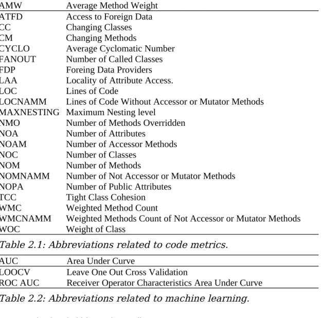
AMW

Average Method Weight

ATFD

Access to Foreign Data

CC

Changing Classes

CM

Changing Methods

CYCLO

Average Cyclomatic Number

FANOUT

Number of Called Classes

FDP

Foreing Data Providers

LAA

Locality of Attribute Access.

LOC

Lines of Code

LOCNAMM

Lines of Code Without Accessor or Mutator Methods

MAXNESTING Maximum Nesting level

NMO

Number of Methods Overridden

NOA

Number of Attributes

NOAM

Number of Accessor Methods

NOC

Number of Classes

NOM

Number of Methods

NOMNAMM

Number of Not Accessor or Mutator Methods

NOPA

Number of Public Attributes

TCC

Tight Class Cohesion

WMC

Weighted Method Count

WMCNAMM

Weighted Methods Count of Not Accessor or Mutator Methods

WOC

Weight of Class

Table 2.1: Abbreviations related to code metrics.

AUC

Area Under Curve

LOOCV

Leave One Out Cross Validation

ROC AUC

Receiver Operator Characteristics Area Under Curve

Table 2.2: Abbreviations related to machine learning.

2.1.2 Metric Threshold for Code Smells

To be able to distinguish and determine if a detected object is of a certain code smell it has to be classified using some metrics from the source code. Such metrics can then be used to set a definition of a code smell within a system. For example, in a rudimentary sense we could define a brain method code smell as a method that has 100 LOC. In a real system such definition would not be generalizable to other systems or even other classes. Therefor it is essential that threshold levels are defined for each metric that constitutes a code smell.

M. Lanza and R. Marinescu defines such metrics in their book for each of the code smells that will be investigated in this study [24]. In their book M. Lanza and R. Marinescu also provides a set of threshold levels for their metrics, statistical and semantical.

2.1.3 Code Smells – Statistical Thresholds

The threshold levels set for each of these defined by Lanza and Marinescu [24]. They performed a statistical survey of 45 java projects and derived the thresholds based on those 45 software systems. The projects varied from 20 000 lines of code up to 2 000 000 lines of code. Both from opensource projects as well as industrial systems.

Based on the findings they calculated an average and standard deviation for the systems. The standard deviation was then used to calculate the low, high and very high values. This was done for each metric to be used [24]. The result of these calculations for java software projects can be seen in Table 2.5.

Low=avg−stdev High=avg+stdev Very High=(avg+stdev)∗1.5

Figure 2.1: Definition

of how the columns for

table 2.3 is calculated.

Statistical Thresholds

Metric

Low

Average

High

Very High

CYCLO/

0.16

0.2

0.24

0.36

LOC/Method

7

10

13

19.5

NOM/Class

4

7

10

15

WMC

5

14

31

47

AMW

1.1

2

3.1

4.7

LOC/Class

28

70

130

195

Table 2.3: Statistical Thresholds for metrics derived from statistical

analysis of 45 java projects [24].

2.1.4 Code Smells – Semantic Thresholds

The semantic metrics are defined not from statistics but are inferred from what the authors consider common knowledge. The used thresholds are normalized to be as easily understandable as possible in the context of setting up filtering statements for the code smells. The inferred thresholds for semantics can be viewed in Table 2.4 and Table 2.5.

Semantic Thresholds Fractions

Numeric Value

Semantic Label

0.25

ONE QUARTER

0.33

ONE THIRD

0.5

HALF

0.66

TWO THIRDS

0.75

THREE QUARTERS

Table 2.4: Semantic Thresholds for metrics fractions to define code

smells [24].

Semantic Thresholds Filter

Numeric Value

Semantic Label

0

NONE

1

ONE/SHALLOW

2 – 5

TWO, THREE/FEW/SEVERAL

7-8

Short Memory Cap

Table 2.5: Semantic Thresholds for metrics naming is arbitrary to

the function, The thresholds have been based on a rudimentary

concept that number 0-7 are part of human short-term memory

[24].

2.2 Code smells

Code smell is a factor when deciding on when and where to refactor in a software system [7][14][15]. Code smell emerges during software development as a part of the technical debt that comes from the trade-off with short delivery times and software quality [6][7]. There are several types of code smell [14].

2.2.1 God Class

God class is refering to a class that has grown too large and tries to do too much, comparable to Fowlers large class code smell [14][24]. This type of class is considered an anti-pattern because when it is present duplicated code and long method code smells will not be far behind [14]. A common practice in object-oriented software architecture is divide and conquer. Each class and method solve its own specific problem but not more. God class is in direct opposition of this practice. God classes also lowers the reusability and understandability of the system [24].

To battle god class code smell it is suggested to divide the class up into more specific methods or classes that target a specific process or state of the software. This can be done by for example extracting the variables from the class and dividing them up into categories and designing classes around those categories instead [14].

To detect god classes using metrics three main concepts can be used [24].

1. If the class accesses the data of other classes often. 2. If the class is large and complex.

3. If there is low cohesion between the methods belonging to the class.

Using metrics to detect code smells will be used to create the dataset for training the ensemble algorithms.

God Class

Metric

Comparator

Threshold

ATFD

>

FEW

WMC

>=

VERY HIGH

TCC

<

ONE THIRD

Table 2.6: God Class metrics definition [24].

If a class fits the metrics given in Table 2.6 then it will be considered a god class in the training dataset.

2.2.2 Feature Envy

Feature envy code smells describes the symptoms of a method that accesses attributes and data of other classes than of its own attributes and data. This could be either through accessor methods or directly. A common occurrence of this is when a method calls another classes or methods getter functions often. This in turn means that the method communicates more with other classes or methods than internally [14] [24].

The easiest and most common fix for this type of code smell is to move the function to be with the data. By doing so the cohesion of the system is enhance since the classes and methods will be more specified for a specific issue. And the coupling becomes looser between methods and the system becomes more modular [14].

To detect feature envy three main concepts can be used [24]:

1. Does the method use more than a few attributes of other classes? 2. Does it use more attributes of other classes than of its own?

3. Does the attribute used belong to very few other classes, is it a small selection of outside classes?

Feature Envy

Metric

Comparator

Threshold

ATFD

>

FEW

LAA

<

ONE THIRD

FDP

<=

FEW

Table 2.7: Feature Envy metrics definition [24].

If a method fits the metrics given in Table 2.7 then it will be considered a case of feature envy in the training dataset.

2.2.3 Brain Method

Brain method is similar to the god class code smell. It centralizes the functionality of a class within one method [24]. In object-oriented software a method should be specialized on a specific task or issue to maximize modularity and maintainability. Which will manifest in tight cohesion and loose coupling. Given a brain method the risk is that it will be difficult to understand and maintain [24].

The detection of the brain method code smell derived from three separate code smells, long methods, excessive branching and many variables [24]. Long functions tend to be difficult to understand for new persons on a project. Difficult to maintain and to reuse [14]. Usually a long function performs more than one function which is undesirable in object-oriented programming [14][24]. This multi-functionality of long functions tends to make the functions more error prone and recurring in refactoring [24]. To combat long methods a common concept is to extract functions from within the long function. To derive new smaller and more specialized functions from the functions performed by the long function [14][24]. Excessive branching occurs when a function uses if-else, and switch statement. The use of such statements are considered to be symptoms of bad object-oriented design [24]. Many variables used code smell is when a function uses many local variables as well as instance variables.

From the identification of these three code smells as the sub-smells of the brain method code smell the detection method derived is following [24].

 Is a function very large?

 Does the function have many branches?  Does the function nest deep?

 Does the function use many variables?

Brain Method

Metric

Comparator

Threshold

LOC

>

HIGH(Class/2)

CYCLO

>=

HIGH

MAXNESTING

>=

SEVERAL

NOAV

>

MANY

Table 2.8: Brain Method metrics definition [24].

If a method fits the metrics given in Table 2.8 then it will be considered a brain method.

2.2.4 Shotgun Surgery

Shot gun surgery is the concept that changing one method or class forces changes to be made in coupled classes and methods [14]. This would mean that if method x and y were coupled and changes were made to method x, we would also need to change y for the software to work [24]. This is referred to as dependencies in this scenario. Because of this it can be easy to miss necessary changes in methods depending on another one and because of that becoming difficult to maintain.

Shotgun surgery code smell can be prevented and refactored in several ways. One such would be to move methods closer to the data. By doing so the methods that would be affected by a change would be closer to each other in the context of the code.

To detect shotgun surgery two main metrics are proposed [24]. 1. If an operation is used by many other operations.

2. If the method is called by many different classes.

Shotgun Surgery

Metric

Comparator

Threshold

CM

>

Short Memory Cap

CC

>

MANY

Table 2.9: Shotgun Surgery metrics definition [24].

If a method fits the metrics given in Table 2.9 then it will consider a case of shotgun surgery in the training dataset.

2.3 Machine Learning Single Model Techniques

There exist many different machine learning algorithms specialised at different tasks and problem domains. Several of which has been used to try identifying code smell in software [2]. However, the investigation into the impact of different and multiple predictors have not been investigated [2].

When designing machine learning algorithms and tools the pre-processing of the data is of high importance since the processed data will be supplying the predictors used for the machine learning algorithm to make predictions and train on.

Machine learning algorithms become efficient to classify and predict certain problems because of the large dataset that the algorithm can train and test on. This is one key factor to why machine learning algorithms can become more efficient than conventional algorithms design by developers. The time to develop the algorithm might be shorter and better return of investment for a developer.

Previously rule based tools have been used to automatically identify code smells in software systems [2]. These tools have been able to identify a subset of code smells within systems. However, the union between tool identified code smell and human identified code small have been small [3]. Because of the rule based nature of code smells machine learning algorithms has proved to be an efficient method of automating code smell identification [2][5]. The three most common single model machine learning methods used to identify code smells have been decision tree, support vector machines, SVM, sequential minimal optimization, SMO and Naive Bayes [10].

2.3.1 Single Model Code Smell Identification

Single model machine learning methods have been able to efficiently identify code smells. From the three most commonly tested single model machine learning algorithm none was among the top two in either systematic literature review. The most effective was JRip, J48, SMO and Naive and random forest models [10][11]. Important to note is that the random forest model is not a single model method but an ensemble of single models. Ensemble techniques is a common method of improving machine learning methods [23]. Ensemble methods were also recommended by two systematic literature reviews as further work [10] [11].

2.3.2 J48

J48 is a decision tree based machine learning model, with focus on information theory. It acts similarly to decision tree models with splitting branches. In the J48 models the splitting of a tree is splitt on the attribute that has the highest information gain.

2.3.3 JRip

JRip is a machine learning model that uses repeated pruning to achieve error reduction of the classifications. JRip adds on conditions to a rule incrementaly until the rule is perfect, having an accuracy of 100%. After a rule set is identified the JRip method prunes the rules into two variants of each rule. This process is then repeated until there are no more left over positives within the training set.

2.3.4 Naive Bayes

Naive Bayes is a machine learning model based on Bayes theorem. Naive Bayes assumes that all the attributes of a class or object is unrelated and independent of eachother. Based on each attribute of a class Naive Bayes calculates a probability of an outcome and uses that probability to classify new instances according to Bayes theorem.

2.3.5 SMO - Sequential Minimal Optimization

SMO is a machine learning method that implements a SVM, Support Vector Machine, model with a more efficient implementation. SVMs define a set of hyper planes based on training on a dataset. These hyperplanes are then used as references for the vectors calculated for each instance in a dataset. The dot product in relation to the hyperplane is used to classify an instance by determining how close to the hyperplane it is. The hyperplane is also used to seperate the instances as a border between the possible classifications.

2.4 Machine Learning Ensemble Techniques

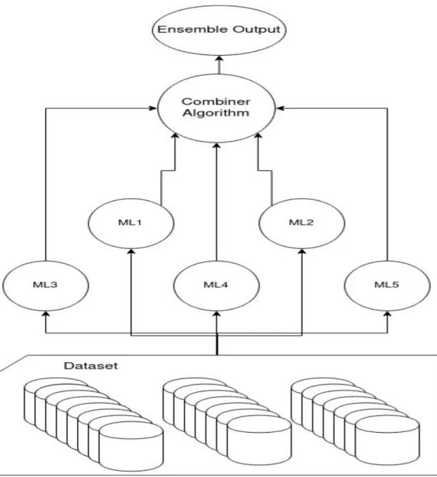
While single model machine learning algorithms can achieve high performances in many areas, they can struggle with more complex data that is imbalanced, high-dimensional or noisy in its nature [16]. The issue derives from the fact that it is difficult for the single model algorithms to capture the full extent or context of the more complex data. To combat this the concept of ensemble models have been used. An ensemble is a set of several single model algorithms either based on the same model or different ones. The set of models then make their own predictions or classifications based on their training. The ensemble then combines the predictions into a singular one for the entire model [16]. The method of combination can vary depending on the ensemble and in turn affect the predicted outcome. The ensemble can also vary depending on the data it is trained on and how the models within the ensemble is trained. During this research the ensemble will be a heterogeneous ensemble, meaning that it is build-up of different classifiers, but they are all trained on the same dataset.

Several challenges exist for single model machine learning algorithms that ensemble techniques can solve. Class imbalance within datasets is a common issue. Class imbalance arises when a class within a dataset has significantly more examples than the other classes in the dataset. This can result in the algorithm favouring the class with more examples. A consequence of this is that the algorithm will then not perform as expected on another dataset where the class balance might be different. Ensemble techniques can prevent this by training the constituent models on a balanced subset of the dataset [23].

Another challenge for machine learning algorithms is the abundance of properties to train upon. When there are a lot of properties the dataset has high dimensionality and will become complex for the algorithm to find generalizable models for predictions. A solution to the issue of high dimensionality is for example attribute bagging [23].

2.4.1 Random Forest

Random forest models is an algorithm based on a metaphorical forest of decision tree models. However, the decision trees within the forest will drop random branches or leaves of the models to find different patterns and produce a variety of rules. The combined output of these trees within the forest is then used as the output from the model. This combination of several single model algorithms makes random forest model an ensemble. The random forest model has achieved high scores in the detection of code smells [10][11]. As an ensemble the random forest model is

considered a voting ensemble for determining the result from the total model as shown in Figure 2.2. During previous studies it was found that the random forest model was among the best of identifying code smells in java projects [10][11].

2.4.2 Voting Ensemble

Voting ensembles uses the outputs of the models within the ensemble to make a vote on their classification. This voting result is then used as the classification for the ensemble.

Within voting ensembles there are several approaches, majority voting and weighted voting. Majority voting is the simplest one where the classification of the ensemble is the option that received a majority of the votes. If there is no majority the ensemble could make a assertive classification. Weighted voting is where better models within the ensembles have more votes or heavier votes. The weighting of the models is up to the researcher.

2.4.3 Stacking Ensemble

Stacking ensembles are where machine learning models' predictions are used as the dataset for another machine learning algorithm. In other terms a machine learning algorithm will train on the output of several other machine learning algorithms to make a prediction of its own. The models used in the stacking will be trained on the dataset at hand independently. And afterwards the outputs of those models will be combined with another algorithm, the combiner. To make up the output of the stacking ensemble as shown in Figure 2.3.

Figure 2.2: The architecure of a random forest ensemble. The

green means positive and red negative. The outcome of this

would therefore be a positive for the classification.

Figure 2.3: Implementation of a stacking ensemble.

2.4.4 Boosting

Boosting is another common ensemble technique used to enhance weak models and reduce their error proneness. Boosting is considered to be an ensemble to decrease the bias of a machine learning algorithm. This is done by trying to train models sequentially, the next model in an area where the previouse model lacked. However, research has shown that boosting can lower the performance compared to individual models [10] [11]. This is speculated to be caused by overfitting of the algorithms. 2.4.5 Bagging

Combines several weak models independently trained in parallel. By doing this the goal is to achieve an ensemble model that is stronger and then the individual weak models composing it. Bagging several weak learners creates a model with less variance since several models will be trained on the same problem.

2.5 Evaluation Metrics – Evaluating Ensemble Performance

To be able to evaluate and compare the results of different ensemble techniques a set of metrics will be used. Theses metrics are defined to measure the performance of a machine learning model, independently if it is an ensemble model or single model. The set of metrics, precision, recall, f-measure, accuracy and AUC ROC are used to ensure as good comparability between models as possible. All ensemble models performance will be evaluated as a combination of these metrics.

2.5.1 Precision

Precision measures the number of true positive predictions made in all of positive instances. Precision becomes the accuracy with which the positive predictions made are actually positive.

P_T=True Positive P_F=False Positive Precision=P_T/

₍

₎

2.5.2 Recall

Recall measures the ratio of all the positives found amongst all of the possible positives. Therefore, recall provides a metric for missed positives that the model could have found and provide input on possible improvements.

P_T=True Positive N_F=False Negative Recall=P_T/

₍

₎

F-measure is a harmonic mean of precision and recall. Since it is possible to have a very good precision score and a terrible recall score, or the reverse. Neither the precision score nor the recall score can tell the whole story of the achieved performance for the model. To give a metric for evaluation that is more telling of the whole model and performance a F-measure is calculated.

P=Precision R=Recall

F − measure=

(

)

(

)

2.5.4 Accuracy

Accuracy is the fraction of percent of the classifications from a model that is correct. From all the predictions made how many where correct. Accuracy does not provide a strong picture or evaluation on itself. With combination of other metrics accuracy does become interesting as an additional performance indicator.

2.5.4 AUC ROC

Area under receiver operator characteristics curve, ROC AUC, has been found to be a good threshold-independent metric for evaluating model performance. The AUC if calculated as a decimal value between 0 – 1. The AUC is computed on the area under the curve that plots the true

positive rate compared to the false positive rate for a given model. In terms of performance an AUC value of 0 is the worst and a value of 1 best [17]. Compared to precision and recall AUC ROC is a threshold-independent metric while the previous are threshold-dependent. In recent studies it has been shown that threshold-dependent metrics e.g. precision and recall, are more prone to bias [18]. Because of this AUC ROC is an important compliment to the precision and recall metrics to ensure less biased evaluation.

2.6 Validation of Ensemble Results

Validation of machine learning model outputs is to ensure that the result is consistent and reproducible. Because of the nature of machine learning training in relation to the dataset there is a risk that the findings may vary depending on the training and testing sets population. To validate the results and give them trustworthiness a set of validation methods can be used. The most common one is cross-validation k-fold which loops over the dataset and trains the models on unique training and testing sets k times. The second one which is more computationally heavy but stronger is leave one out cross-validation.

2.6.1 Cross-validation K-fold

K-fold cross-validation is a commonly used method of validating a model for its performance. And is widely used within the research community to assess and validate models trained for research [10][11]. K-fold cross-validation works by dividing up the dataset into K random subsets of data. Then trains the model with K – 1 subsets of the data and afterwards validates the model with subset K. This is repeated until every subset is used as training and testing. This way of validating a model is sufficient as an initial validation of the model, however it is not exact or unbiased enough to be the final validation of an important model [10][11][17]. This is because there is a small factor of bias that is possible from the validation [10][17].

2.6.2 Leave-one-out Cross-validation

An improved version of the k-fold cross-validation is the leave-one-out cross-validation, LOOCV. LOOCV improves over the cross validation by adding another fold on top of the k-fold. E.g. if the cross-validation would be 10-fold, dividing the dataset into 10 subsets and testing and training for each. The LOOCV would perform the 10-fold 10 times to ensure that the randomisation of the initial subsets is not a factor in the performance of the model [17].

Because of the added fold with LOOCV it is substantially slower and demands more computational power. Therefore, it is suiTable to perform K-fold cross-validation initially to validate models. However, when the final validation is to be done it more rigorous to use LOOCV for validation to ensure that the validation is as unbiased as possible [17].

2.7 Tools for experiment configuration and evaluation

To be able to perform and create the ensemble methods and reliably evaluate and validate them a set of tools is needed. Any machine learning algorithm needs to be trained on some data that represents the intended population to use it on. This dataset needs to be labelled and accessible. To setup and run the machine learning algorithms a framework is

needed, graphical or not. And to calculate the evaluation metrics a unified framework is necessary.

2.7.1 Qualitas Corpus Dataset

Qualitas Corpus is a dataset containing curated open-source java projects. The purpose of Qualitas Corpus is to ensure that there is a common and usable dataset for empirical studies on software artefacts. The dataset is maintained and curated by Ewan Tempero, The University of Auckland. The purpose of the dataset is to ensure a common and repeatable source of data for research regarding code and software systems. The dataset contains 112 java systems that are curated with metrics. These metrics include cohesion, lines of code, etc.

2.7.2 Weka

Weka is a open-source machine learning software that can be used as a graphical interface, through terminal or java API. Weka was the most used tool found in two systematic literature reviews [10][11]. Weka works as a tool-bench where the interaction between data and machine learning algorithms is assisted. There are also tools for data pre-processing. Weka has the tools to implement the validation and leave one out cross-validation. It can also for each model calculate the evaluation metrics, precision, recall, f-measure, accuracy and AUC ROC. By having this in a unified and opensource tool the reproducibility of the study is increased, and transparency of process ensured.

2.7.3 WekaNose

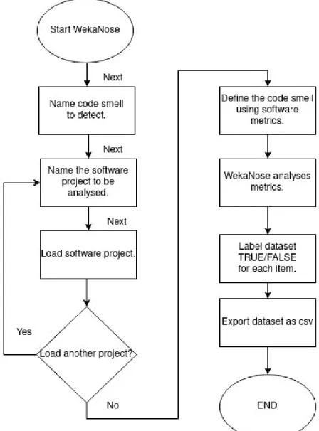
WekaNose is an open-source tool developed to ensure that the definition of code smells within different heterogenous datasets will use the same metrics and therefore be comparable over studies. WekaNose uses a given dataset of executable java code and according to a definition of a code smell given by the researcher creates a testing set to be used for machine learning algorithms. WekaNose is used as a plugin to the machine learning workbench Weka.

The definition of a code smell is provided by the researcher. The definition should be based on software metrics available in the dataset. The dataset of code smells from WekaNose is used as a test oracle for the machine learning algorithms. The process for creating a dataset with WekaNose is shown in Figure 2.4. The dataset is created by gathering a set of items that is close to the definition set by the researcher. After the dataset is gathered from the analysed projects the researcher must go through the data and label items either “TRUE” or “FALSE” depending on if the item is of a code smell or not. First after this step is performed the dataset can be used for training machine learning models.

Figure 2.4: The process of creating a dataset for

machine learning using WekaNose.

2

Method and implementation

In this section the design of the experiments and the process of preparing the experiments is described.

3.1 Experimental Computer Science

Experiments in computer science is an approach to research that is called for by multiple instances and articles. There is a considered lack of experiments within the field of computer science compared to other domains of research [9][30][31]. There are two identified major benefits of doing experimental computer science. Through testing of algorithms or programs experiments help creating databases of knowledge, tools and methods of similar studies. Secondly experiments can lead to unexpected results resulting in an effective way of eliminating methods and hypotheses based on the experiment results [30]. To enable good experimental computer science four qualities of a good experiment has been defined, reproducability, extensability, applicability and revisability [29]. Reproducability ensures that the study can be reproduced independently by another research team or institution. Extensability means to make the results comparable to other studies and research. Applicability is the quality of using realistic parameters and that the experiment should be easy to configure. Revisability, that if an experiment does not give the expected outcome, the experiment should help explaining why.

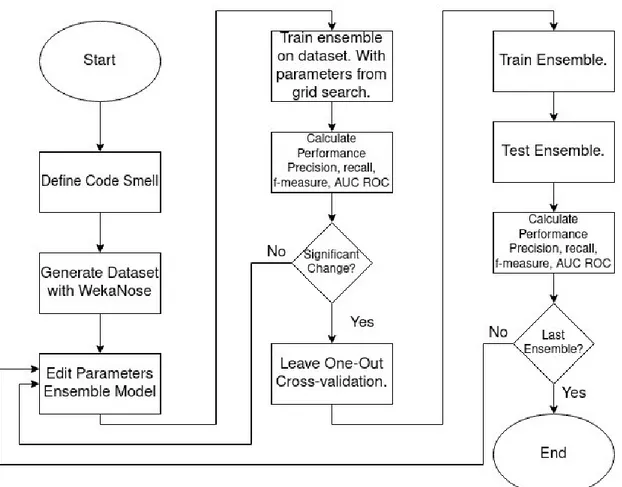
3.2 Experiment Design Research Question One

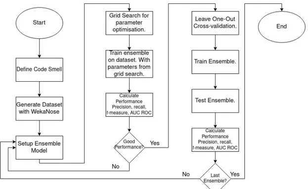
The code smells to be used for the research will be defined by the researcher in the WekaNose tool based on the existing metrics in Qualitas Corpus. WekaNose will then by following these definitions create a dataset. The dataset derived by WekaNose will then be used as training set as well as test oracle.

After the datasets has been created the ensembles will be trained on the derived metrics from Qualitas Corpus software systems codes to identify the targeted code smells. Initial training and validation of an ensemble technique will be done by k-fold cross-validation, CV. CV will be used as the initial validation method to lower the computational cost. When an ensemble method has proven good performance with CV LOOCV will be performed. LOOCV will be used to ensure as low bias as possible for the final results of the ensembles. The ensemble will be tested against the dataset of code smells generated by WekaNose. The outcome of the LOOCV validation will then be used to calculate the evaluation metrics, precision, recall, f-measure, accuracy and AUC ROC. The calculated performance metrics will be used as the score for an ensemble and provide the metrics that will be compared with the other ensembles. This process will be repeated for each of the designated ensemble techniques before comparative evaluation between them are done. The outcome for RQ1 will be the ensemble method with the best score from the evaluation metrics, as seen in Figure 3.2.

Figure 3.1: The process of experimentation for research question

one.

3.2.1 Creating the Datasets

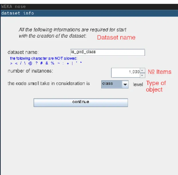
The datasets created and labelled in this process will be used for research question two as well. To create the datasets to be used for each code smell there is a set of steps that need to be performed for each of them. First the naming of the dataset, the number of items to be included in the dataset and the type of object investigated, method or class, as shown in Figure 3.2.

Figure 3.2: The first step to creating a dataset for training models to

identify the god class code smell. The red text has been added to

highlight information.

After setting the initial parameters of the dataset the libraries used to gather the source code to be analysed must be loaded and processed. This process is a labor intensive process that requires the researcher to identify which libraries from the code base that can be used and what parts of it that can be used. Not all projects within the Qualitas Corpus dataset of opensource projects could be used due to compatibility issues. To load a project, path to the source of the project had to be defined as well as the path to the libraries need to execute it. This is shown in Figure 3.3.

Figure 3.3: Showing the interface for loading each of the java

projects. The red text has been added to highlight information.

The loading time of a project has a wide range from five seconds to 70 seconds. In total for each of the code smells 57 projects were loaded. Due to an incompatibility issue with some of the projects within the Qualitas Corpus dataset and the process of WekaNose there was a need for identifying compatible projects. For each of the projects within Qualitas

Corpus the manual process of testing each layer of folder structure had to be done. This was done three independent times with the outcomes recorded in an excel file. This excel file was then used as reference to ensure that the same projects were loaded in the same manner each time a dataset was created. The projects and their relative path can be seen in appendix A. When all the projects have been successfully loaded the next step is to supply WekaNose with the advisors and definitions of code smell to look for within the loaded projects, this is shown in Figure 3.4.

The advisors are used by WekaNose to analyse the code of the loaded projects and gathering items from the projects that either fit the definition provided or are close. As with the case of the TCC advisor, the actual value we are looking for is objects with a TCC lower than 1/3 however due to limitations in WekaNose the advisor cannot be set lower than one. WekaNose will output a csv file with items that fit the advisors and are close to the advisors on both ends. This ensures that there will be items that does not fulfil any of the advisors for the code smell as well as items that fulfil all of them or a set of them.

After the dataset have been outputted by WekaNose the data is unlabelled. The labelling has to be done manually by the researcher according to the definition of the code smell at hand. The process was automated to a certain degree by using if statements within librecalc. The

Figure 3.4: An example of the interface with advisors used to

gather the dataset items for god class code smell.

if statement followed the definition set in the associated Table of definition for each code smell.

To achieve balance between positive and negative items in the datasets created for the code smells positive or negative items were removed until a partitioning of 1/3 positive and 2/3 negative was achieved. This is a common approach to balance unbalanced datasets [27].

3.2.3 Models Considered in Implementation.

The models that will be used in the implementations will be based upon which models have achieved the best result as single models in previous studies [10][11][26]. The best performing model in several of the previous studies have been JRip models. Because of this the JRip model will be used in the experiments for research question one. The second-best model has been random forest in several studies. However due to the fact that it is a model of the voting ensemble method it will not be considered in this part as a single model. Another contender has been the J48 model, a type of decision tree model. Because of the good performance for J48 in previous studies it will be used in the experiments. Naive Bayes and SMO have shown strong performance for certain code smell in previous studies [10][26]. Because the code smells are included in the ones use in this study they will also be considered for the experiments. The machine learning models selected here will be used to build up the basis for the stacking and voting ensembles. As well as the combiner methods for the stacking ensemble. Theses code smells will also each be tested with bagging and boosting methods of ensembles.

3.2.2 Experiment Setup

Each experiment will be performed for all the four selected code smells. These code smells will be represented in four distinct manually labelled datasets. Each row in the datasets represents one case of a possible code smell from a set of open sources java projects. Each data item has 30 code metrics that the machine learning algorithms can consider. The reason for this experimental approach is because it is called for within the community of data science as well as provides direct results towards an issue [9]. It has been shown that in code smell detection more metrics provides better models. The datasets have been resampled to have a ratio of 1/3 positive and 2/3 negative items to the total number of items. This is a common ratio considered for good training material for the models [27]. The models, ensemble and single models are trained and evaluated one at a time using Weka’s experiment mode. However within in one session there will at times be more than one iteration of the ensemble. Weka has the capability to run all the models in the same session. Doing so takes significantly longer and would lower the possible amount of iterations to be done.

3.2.4 Establishing Frame of Reference

To ensure the reproducibility and the quality of the dataset and general setup of the experiment a test according to previous studies will be performed. The results achieved by two previous studies with the machine learning models random forest and Jrip were 91.29% and 97.44% respectively [10][19][26]. These two studies were also performed on the Qualitas Corpus dataset and would therefore be ideal for comparison and validation. By performing test runs with random forest

and Jrip models on the created dataset the expected outcome would be close to the results by the previous studies [10][26]. The frame of reference will use the same validation methodology and datasets as the other experiments performed within this study to provide insight into the validity of the process and setup.

3.2.5 Recording of Results

The results from the classifications and experiments are gathered as experiment data within Weka. From Weka the data is transferred to a librecalc document for further processing. All the measurements from Weka are done with a t-test with a significance of 0.05. Within openoffice calc the data for each dataset, ensemble model and code smell is grouped up and processed into an average for that specific model. This processed data is later used to compare different models to each other. To compare the data charts are created to visualise the results.

3.3 Experiment Design Research Question Two

The code smells to be used for the research will be defined by the researcher in the WekaNose tool based on the existing metrics in Qualitas Corpus. WekaNose will then by following these definitions create a dataset. The dataset derived by WekaNose will then be used as training set as well as test oracle.

After the datasets has been created the ensembles will be trained on the derived metrics from Qualitas Corpus software systems codes to identify the targeted code smells. The parameters of the ensemble will be modified iteratively. The purpose of this is to identify parameter sensitivity if any exists within in the ensemble. Initial training and validation of an ensemble technique will be done by k-fold cross-validation, CV. CV will be used as the initial validation method to lower the computational cost. When a ensemble method has proven good performance with CV LOOCV will be performed. LOOCV will be used to ensure as low bias as possible for the final results of the ensembles. The ensemble will be tested against the dataset of code smells generated by WekaNose. The outcome of the LOOCV validation will then be used to calculate the evaluation metrics, precision, recall, f-measure and ROC AUC. The calculated performance metrics will be used as the score for an ensemble and provide the metrics that will be compared with another ensemble.

If the difference between two or several ensemble techniques from RQ1 is small, then the two closest ensembles will be targets for a sensitivity analysis according to the description above. This is to ensure and investigate if one of the ensembles have an advantage over the other considering parameter dependents, as seen in Figure 3.2.

3.3.1 One-At-a-Time Sensitivity Analysis

To be able to provide an as unbiased evaluation of parameter change to the model one-at-a-time, OAT, sensitivity analysis will be performed. OAT is a common approach when the outcome of system or model is thought to be impacted by one or more factors [28]. The process of OAT is to have all factors for a model at their nominal values. Change one factor and leave the others in their nominal values. Record the result. Reset the changed factor to its nominal value. The next cycle is then to change the value of another factor and record the result. By doing this it is possible to identify factors that have high influence on the system and propose changes according to those findings [28]. The sensitivity analysis will be done on the AUC ROC score for the model to use as comparative measurement.

3.4 Experiment Environment

The experiments where performed on a desktop pc with a NVidia GTX 970 GPU, Intel(R) Core(TM) i7-6700 CPU @ 3.40GHz, 16GB of ram. Operating system was arch Linux rolling release on kernel 5.6.5-arch3-1.

Figure 3.5: The process of experimentation for research question

one.

3

Results and Findings

In this section the data gathered is described with the experiments performed and the outcome of the experiments.

4.1 Result From Dataset Creation

From the process of creating datasets one dataset was created for each code smell. The datasets where from the same projects however the distribution of code smells per java project varied. When the labelling process was completed for the data items gathered there was a significant difference between the ratio of occurring code smells. For example, in the case of the god class code smell as well as the shotgun surgery there was over 200 positive data items, 228 and 245 respectively. While for feature envy and brain method there were 78 and 73. After the datasets were balanced according to the 1/3 positive and 2/3 negative ratio commonly used the metrics shown in Table 4.1 were achieved [27].

Nr of projects Positive Items Negative Items Total Items Ratio

God Class

57

228

456

684

0.33

Feature Envy

57

78

156

234

0.33

Brain Method 57

73

146

219

0.33

Shotgun

Surgery

57

245

490

735

0.33

Table 4.1: Data item metrics for the created datasets to be used for

the experiments.

4.2 Result for Establishing Frame of Reference

Here the results of the attempted reproduction of two experiments from previous studies on single model machine learning is presented. The achieved f-measures from this study for the comparison and establishment of the validity of the setup is displayed in Table 4.2.

JRip Pruned

JRip Unpruned

Random Forest

F-Measure Std. Dev. F-Measure Std. Dev.

F-Measure Std. Dev.

Brain Method 0.890

0.150

0.930

0.130

0.910

0.110

Feature Envy

0.960

0.090

0.970

0.080

0.890

0.120

God Class

0.980

0.070

0.980

0.080

0.960

0.170

Shotgun

Surgery

1.000

0.000

1.000

0.000

0.960

0.040

F-Measure Avg.0.958

0.970

0.930

Std. Deviation

Avg.

0.078

0.073

0.110

Table 4.2: Single model result from establishing frame of reference

run performed in this study.

The results achieved with the setup prepared for this study the results are similar and close to the frame of reference results from the two selected previous studies with their best models. The difference and similarities considering the F-Measure is shown in Figure 4.1. The results from this experiment compared to the previous studies used as reference are close and within the standard deviation of each metric.

4.3 RQ 1 – Results

Here the data gathered from the training of the ensemble models is presented.

4.3.1 Stacking Ensemble

Here the results of the stacking ensembles for research question one is presented. The results for each combiner method are very close to the other combiner method that have most in common. In this case Jrip and J48 share similarities and Naive Bayes and SMO share some similarities. However, the distinction becomes clearer when considering the accuracy and AUC ROC scores.

Average of Evaluation Metrics

F-Measure

Precision

Recall

Accuracy

AUC ROC

Jrip

0.975

0.988

0.953

95.638

0.960

J48

0.975

0.988

0.953

95.753

0.963

Naive Bayes

0.978

0.993

0.950

95.908

0.980

SMO

0.978

0.993

0.950

95.895

0.965

Table 4.3: The average metrics for the stacking ensembles.

The results in Table 4.3 are used to produce comparative bar charts between the different combiner methods. Using these Figures to

Jrip Random Forest Jrip pruned

0 0.2 0.4 0.6 0.8 1 1.2 0.97 0.97 _{0.93 0.96} 0.91

Frame of Reference

Machine Learning Model

F -M e a su re

highlight differences and similarities in scores for the evaluation. These Figures also provide the basis for selecting a strongest method from the stacking ensemble experiments. The F-Measure that is shown comparing the combiner methods for the stacking ensemble show distinct similarities, in Figure 4.2, between the models that share similar approaches to classification. Given that the single models that constitutes the stacking ensemble are the same for each combiner method there is an expectation that differences should only be based on the combiner methods used. In the case of the F-Measure the similarities between the combiner methods is instead made clear. JRip is a rule-based model, J48 is a tree-based model. Which share a lot of similarities in the approaches that they produce. The Naive Bayes and SMO also shares similarities, but not to the extent that JRip and J48 does.

In Figure 4.3 showing the accuracy of the methods, there is a small difference between the methods. The difference between the methods is relatively small and does not necessarily provide a clear strongest method.

Figure 4.2: F-Measure for stacking ensembles with JRip, J48, Naive

Bayes.

Figure 4.4 shows the AUC ROC scores in relation to the other methods of stacking combiners. For the stacking ensemble this is the metrics that provides a clear distinction between models. With the combination of the scores for F-Measure, accuracy and AUC ROC the Naive Bayes as combiner model must be considered the strongest method from these results.

Figure 4.3: Accuracy for stacking ensembles with JRip, J48, Naive

Bayes.

4.3.2 Voting Ensemble

Here the results and data gathered for the voting ensembles are presented. The results here are showing the comparisons and the results gathered from the experiments that was performed. The summary of the experiment data is shown in Table 4.4.

Average for Voting Ensemble

F-Measure Precision

Recall

Accuracy

AUC ROC

Average of

Probabilities

0.933

0.938

0.965

92.460

0.975

Majorit Voting

0.948

0.933

0.963

92.860

0.915

Product of

Probabilities

0.955

0.935

0.978

81.880

0.860

Table 4.4: The average evaluation metrics for the voting ensemble.

Shown in Figure 4.5 the F-Measure of the voting method of product of probabilities has the highest F-Measure score.

Figure 4.4: AUC ROC for stacking ensembles with JRip, J48, Naive

Bayes.

For the accuracy metrics average of probability and majority voting shows, in Figure 4.6, a significant better score compared to the product of probabilities which had a high F-Measure. F-Measure score weighs higher than the accuracy for these experiments, but the methods considered strongest will be based on the combination of all three metrics.

Figure 4.5: F-Measure for voting ensembles with JRip, J48, Naive

Bayes.

Figure 4.6: Accuracy for voting ensembles with JRip, J48, Naive

Bayes.