2005:21 DECOVALEX III PROJECT Thermal-Hydrological Modeling of the Yucca Mountain Project Drift Scale Test

SKI Report 2005:21

Research

DECOVALEX III PROJECT

Thermal-Hydrological Modeling of the

Yucca Mountain Project Drift Scale Test

Task 2A Final Report

Compiled by:

Robin N. Datta

February 2005

With contributions from: Sebastia Olivella Claudia Gonzalez Antonio Gens Miguel Luna Ronald T. Green Scott L. Painter ISSN 1104–1374 ISRN SKI-R-05/21-SE

SKI Project Number XXXXX

SKI Report 2005:21

Research

DECOVALEX III PROJECT

Thermal-Hydrological Modeling of the

Yucca Mountain Project Drift Scale Test

Task 2A Final Report

Compiled by:

Robin N. Datta

Bechtel SAIC Company, Las Vegas, USA

February 2005

With contributions from: Sebastia Olivella¹ Claudia Gonzalez¹ Antonio Gens¹ Miguel Luna¹ Ronald T. Green² Scott L. Painter²

¹University Polytechnique of Catalina, Spain

This report concerns a study which has been conducted for the DECOVALEX III Project. The conclusions and viewpoints presented in the report are those of the author/authors and do not necessarily coincide with those of the SKI.

Foreword

DECOVALEX is an international consortium of governmental agencies associated with the disposal of high-level nuclear waste in a number of countries. The consortium’s mission is the DEvelopment of COupled models and their VALidation against EXperiments. Hence theacronym/name DECOVALEX. Currently, agencies from Canada, Finland, France, Germany, Japan, Spain, Switzerland, Sweden, United Kingdom, and the United States are in DECOVALEX. Emplacement of nuclear waste in a repository in geologic media causes a number of physical processes to be intensified in the surrounding rock mass due to the decay heat from the waste. The four main processes of concern are thermal, hydrological, mechanical and chemical. Interactions or coupling between these heat-driven processes must be taken into account in modeling the performance of the repository for such modeling to be meaningful and reliable.

The first DECOVALEX project, begun in 1992 and completed in 1996 was aimed at modeling benchmark problems and validation by laboratory experiments. DECOVALEX II, started in 1996, built on the experience gained in DECOVALEX I by modeling larger tests conducted in the field. DECOVALEX III, started in 1999 following the completion of DECOVALEX II, is organized around four tasks. The FEBEX (Full-scale Engineered Barriers EXperiment) in situ experiment being conducted at the Grimsel site in Switzerland is to be simulated and analyzed in Task 1. Task 2, centered around the Drift Scale Test (DST) at Yucca Mountain in Nevada, USA, has several sub-tasks (Task 2A, Task 2B, Task 2C and Task 2D) to investigate a number of the coupled processes in the DST. Task 3 studies three benchmark problems: a) the effects of thermal-hydrologic-mechanical (THM) coupling on the performance of the near-field of a nuclear waste repository; b) the effect of upscaling THM processes on the results of performance assessment; and c) the effect of glaciation on rock mass behavior. Task 4 is on the direct application of THM coupled process modeling in the performance assessment of nuclear waste repositories in geologic media.

Task 2A of DECOVALEX III entails modeling the thermal-hydrologic (TH) response of the DST during the heating and cooling phases of the test to predict the temperature distributions and the movement of rock moisture in the test block at various times. The predictions are subsequently compared with the measurements of temperatures and saturation and are analyzed. The insights/understandings gained allow refinements/adjustments to be made to the conceptual model. This process is expected to eventually result in the development of a robust, validated TH model, which can be the basis for assessing the performance of a repository.

This Task 2A Final Report largely subsumes the Interim Report of February 2002 as well as documents the modeling and comparative analyses done by the research teams subsequently. Lanru Jing Fritz Kautsky Juan-Carlos Mayor Ove Stephansson Chin-Fu Tsang

Summary

Task 2A concerns coupled TH modeling of the DST test at Yucca mountain, with given results for geologic, thermal, mechanical, hydrologic, and mineralogic and petrologic characterization, as-built configuration of the test block of DST, including locations of various sensors and measuring instruments and the plans for heating and cooling, including expected heater powers at various times, and requiring predictions for distributions and evolutions of the temperature and saturation fields. Three teams of ENRESA (Spain), DOE (USA), and NRC (USA) teams participated the task with different approaches, using FEM code Bright with a double porosity structure

(ENRESA), a FDM code MULTIFLO with a dual continuum approach and an active fracture model (NRC) and a FDM code TOUGH 2 with a dual permeability approach (DOE), respectively.

Based on the results of the temperature and moisture distributions and temperature histories, it can be concluded that in general, the three models capture the TH response of the DST fairly well, although there are some differences between the teams’ results. Conduction is the dominant heat-transfer mechanism in the fractured unsaturated rock in the DST, especially in the sub-boiling regime. However, the pore water plays an important role near the boiling point as it goes through cycles of vaporization and condensation causing the so called pipe effect. A characteristic signature of heat-pipes – a short lull in the rise of temperature– was captured by all three teams.

The 2D modeling of the DST carried out by the ENRESA team initially was characterized by very little diffusion of vapor because the tortuosity factor was set at a low value of 0.05 and is referred to as the ND (No Diffusion) case. The recent 3D model with a tortuosity factor set at 1 and a vapor diffusion enhancement coefficient allows maximum vapor diffusion and is referred to as the MD (maximum diffusion) case. Comparative analyses of the modeling results for ND and MD cases lead to the conclusion that diffusion of vapor play an important role in flow and transport in the dry-out zone, since vapor mass fraction reaches its maximum in that region. Vapor flows by advection and by vapor diffusion/dispersion. Advection is very efficient in the high permeability fractured rock; however, diffusion is also a very efficient transport mechanism due to the high diffussivity of vapor in air.

The NRC research team examined two grid block sizes of 04 m and 5.0 m as well as two infiltration rates and the dual permeability model (DKM) with and without the active fracture model (AFM). An increase in model block size allowed relatively large infiltration rates (3.0 mm/yr) while maintaining a moderate ambient matrix saturation of 0.90. There was significant difference in the predicted matrix saturations between the small block model and the large block model as indicated by the larger dry-out zone in the small block model especially at four years after the start of heating.

The sensors in borehole 160, located between two wing heaters, display a wide variety of responses depending on their location with respect to the heaters. The ones located directly above the wing heaters exhibit strong thermal perturbation. Both measured and simulated temperature results have relatively short heat-pipe signals, suggesting that pore water is boiled off in a relatively short time period because of close proximity to the heaters.

Content

Page

1 Yucca Mountain Project Drift Scale Test 1

1.1 Yucca Mountain Project Drift Scale Test 1

1.2 Test setting and test facility 2

1.3 Measurements made 3

2 Task 2A – thermal hydrologic simulation 5

2.1 Task definition 5

2.2 Task 2A research teams 5

3 Modeling of Drift Scale Test thermal-hydrologic (TH) response 6

3.1 ENRESA research team’s TH modeling 6

3.2 NRC research team’s TH modeling 32

3.3 DOE research team’s TH modeling by using code TOUGH 52

4 Discussion and conclusions 72

References 74

1. Yucca Mountain Project Drift Scale Test

1.1 Yucca Mountain Project Drift Scale Test

The DST in Yucca Mountain in Nevada, USA is a large scale, long term field thermal test being conducted for the U.S. DOE. In the DST a ~5 m diameter drift, ~ 50 m long is being heated by electrical heaters to study the response of the surrounding rock mass to the heating and subsequent cooling. The test is an integral part of DOE’s program of site characterization at Yucca Mountain to assess whether the mountain is suitable site for a repository for the disposal of high level nuclear waste and spent nuclear fuel. In Task 2 of DECOVALEX III project the DST is a test case in the process of developing and validating coupled process models.

1.1.1 Purpose and test objective

In the broadest sense the primary purpose of the DST is to develop a thorough understanding of the coupled thermal (T), mechanical (M), hydrologic (H), and chemical (C) processes in the rock mass immediately surrounding the proposed repository because of the decay heat from the nuclear waste. To achieve this primary purpose a series specific sub-tier test objectives are established, categorized around the four principal processes of concern. These test objectives are:

Thermal

‰ Measure the temporal and spatial distributions of temperature

‰ Evaluate influence of heat transfer modes

‰ Investigate possible formation of heat pipes

‰ Determine rock mass thermal properties

Mechanical

‰ Measure rock mass mechanical properties

‰ Evaluate ground support response under controlled conditions

‰ Measure drift convergence at elevated temperatures

‰ Observe effect of thermal loading on prototypical ground support

systems and overall room stability

Hydrological

‰ Measure changes in rock saturation

‰ Monitor the propagation of drying and subsequent re-wetting, if any,

including potential condensate cap and drainage

‰ Measure changes in bulk-permeability (pneumatic)

‰ Measure drift-air humidity, temperature, and pressure

Chemical

‰ Collect and analyze samples of water and gas

‰ Analyze changes in typical waste package material left in the heated drift

‰ Observe changes in water and mineral chemistry from drying and reflux

1.2 Test setting and test facility

A description of the setting of the DST and the test facility can be found in Datta et al, 1999 which is the basis of the following paragraphs.

Yucca Mountain, approximately 135 kilometers northwest of Las Vegas, Nevada is part of a series of north-trending ridges in the Great Basin physiographic province of North America. The mountain is underlain by 1000 to 1500 meters of Tertiary volcanic tuffs, formed from the ash of eruptions occurring between 8 and 16 million years ago. The volcanic tuffs are generally bedded, separated in beds that are generally non-welded to densely welded, and in addition, some are devitrified and others are vitric. The proposed repository horizon is within a sequence of beds, up to 350 meters thick, of moderately to densely welded devitrified tuff known as the Topopah Spring Tuff of the Paintbrush Group. The sub-units of the Topopah Spring Tuff are based primarily on the abundance of lithophysae which are cavities with dimensions on the order of millimeters to hundreds of millimeters, formed due to the presence of gases in the cooling ash flows. The presence or absence of lithophysae can have a pronounced effect on the mechanical and hydrologic properties of the rocks.

Topopah Spring Tuff is divided into four sub-units: the upper and lower lithophysal and the middle and lower non-lithophysal. The geologic symbols for the upper and lower lithophysal sub-units are Tptpul and Tptpll respectively while those for the middle and lower non-lithophysal sub-units are Tptpmn and Tptpln respectively. The lower non-lithophysal sub-unit (Tptpln) is stratigraphically the lower most, overlain by Tptpll, Tptpmn, and Tptpul in that order. The bulk of the proposed repository will be located in the lower lithophysal (Tptpll) sub-unit, with small portions in the middle and lower non-lithophysal sub-units. In the hydrologic stratigraphy of the Yucca Mountain area, the symbols for these sub-units of Topopah Spring Tuff are tsw33, tsw34, tsw35, and tsw36 with tsw36 being the lower most and tsw33 being the upper-most, corresponding to Tptpln and Tptpul respectively.

The DST is located entirely in the middle non-lithophysal sub-unit of Topopah Spring Tuff which is represented by Tptpmn or tsw34. These geologic or hydrologic symbols are frwquently employed in this report to specify the beds.

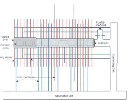
The DST consists of a 47.5m long, 5m diameter drift heated by nine canister heaters, each 1.7m diameter, 4.6m long, placed on the floor of the drift. Additional heat is supplied by 50 rod heaters, referred to as “wing heaters” inserted into horizontal boreholes drilled into each sidewall. (Figure 1-1). The drift cross-section and the canister heaters are approximately the sizes of drifts and waste packages, respectively, being currently considered for the potential repository. The wing heaters are used to simulate the heat that would come from adjacent drifts in a repository, and thus provide better test boundary conditions. Each canister heater can generate a maximum of 15kW. The wing heaters are each 10 meters long, and have inner and outer segments that can generate 1145W and 1719W, respectively. Rockbolts and wire-mesh are installed as ground support along the entire length of the Heated Drift. In addition, the final 12.5m length of the drift is supported by a cast-in-place concrete liner to observe the performance of a concrete-lined drift at elevated temperatures. An Access/Observation Drift excavated parallel to the Heated Drift, and a perpendicular Connecting Drift are constructed around the periphery of the test block (Figure 1-1). The heated length of the drift is isolated from the Connecting Drift by an insulated thermal bulkhead. The bulkhead is not a pressure bulkhead. This means that some heat exchange by convection through the bulkhead will occur. Approximately 3300meters of boreholes are drilled from the Heated Drift, the Connecting Drift and the Access/Observation Drift

into the test block (Figures 1-1, 1-2, and 1-3) to house the wing heaters and approximately 3500 sensors of various types. By the end of the heating phase of the test

extending over four years, approximately 15,000 m3 _{of rock will be heated above 100}

degree Celcius. For complete and full descriptions of the DST, refer to the reports, “Drift Scale Test Design and Forecast Results” (CRWMS M&O, 1997) and “Drift Scale Test As-Built Report” (CRWMS M&O, 1998).

1.3 Measurements made

The following measurements are being made or were planned to be made in the DST:

1. Heater Power

2. Rock temperature by thermocouples and resistance temperature devices 3. Displacement in rock by multiple borehole extensometers

4. Deformation of concrete lining by convergence monitors 5. Strain in concrete by strain gages

6. Moisture content of the rock by neutron logging

7. Moisture content of the rock by electric resistivity tomography (ERT) 8. Moisture content of the rock by ground penetrating radar (GPR) 9. Acoustic or microseismic emissions

10. Relative humidity, temperature, and air pressure in sections of boreholes isolated by packers

11. Relative humidity, temperature, and air pressure in the Heated Drift and outside

12. Changes in fracture permeability (k) by pneumatic methods (air permeability) and gas tracer tests

13. Analyses of gas and water samples collected from the test block

14. Thermal conductivity and diffusivity by REKA (rapid evaluation of K and alpha) probe

15. Periodic video and infrared images of the inside of the Heated Drift 16. Rock mass modulus of deformation by the plate-loading test

17. Temperature on non-rock surfaces such as heaters, bulkhead, cable-trays, etc. using thermocouples

18. Mineralogic-petrologic characteristics of the rock before and after the test 19. Thermal, mechanical, and hydrologic properties of intact rock samples

measured in the laboratory, before and after the test

In addition to the above, coupons of candidate materials for the waste container, cylindrical samples of concrete used for the cast-in-place liner, and native microbes have either been left in the Heated Drift or injected into the test block to study the effects of prolonged heating and cooling on them.

An approximately 6000 channel, automated data collection system (DCS) records measurements on an hourly basis. The DCS scans and records the readings of temperature, humidity, air pressure, MPBXs, strain gages, convergence monitors, and current and voltage for heater power. Other measurements, referred to as active testing, such as air-K measurements, neutron logging, ERT, acoustic emission, GPR, and REKA probe measurements are recorded periodically using independent data acquisition systems.

Figure 1-1.Location of the Wing Heaters, Canister Heaters and Instrument Holes in the Drift Scale Test

Figure 1-2. Cross-Section parallel to the Heated Drift

Figure 1-3.Cross-Section Orthogonal to the Heated Drift

2. Task 2A – Thermal hydrologic simulation

Task 2 of the DECOVALEX III project is centered around the DST. There are four sub-tasks in Task 2 to study the three heat-driven coupled processes of interest. Task 2A is to study the TH response of the test block, while 2B/2C and 2D are to study the THM/TM and THC responses respectively.

2.1 Task definition

The definition of Task 2A is quoted below from the Task 2 Plan of DECOVALEX III.

Given:

a. Results of geologic, thermal, mechanical, hydrologic, and mineralogic and petrologic characterization of the test block of the DST

b. As-built configuration of the test block, including locations of various sensors and measuring instruments

c. Plans of heating and cooling, including expected heater powers at various times

Tasks:

1. Predict the time-evolution of temperature distribution in the test block; a suitable time Interval such as 10, 30, 50, or 100 days may be used

2. Predict the time-evolution of the changes in the saturation of the rock; a time interval of 10,30, 50, or 100 days may be used. Changes in the saturation can be predicted relative to the initial ambient saturation

3. Prepare Interim report documenting the results of the initial predictive analyses

4. Compare predicted temperatures and saturations with measured values. Perform comparative/interpretive analyses and refine conceptual and mathematical models, if necessary

5. Perform Phase II thermal-hydrologic modeling using refined model and actual heating i.e. measured heater outputs

6. Perform final comparative/interpretive analyses using Phase II modeling results and measured temperatures and saturations

7. Prepare Task 2A Report

2.2 Task 2A research teams

Besides the U.S. DOE’s Office of Repository Development (ORD) formerly known as Yucca Mountain Site Characterization Office (YMSCO), the participants in Task 2A are ENRESA of Spain andd the NRC of the United States. The research team of ENRESA is led by Prof. Sebastia Olivella of the UPC in Barcelona, Spain. Ronald Green of the Center for Nuclear Waste Regulatory Analyses of the Southwest Research Institute in San Antonio, Texas leads the NRC’s Task 2A research team. The DOE’s research teams are led by Robin N. Datta.

3. Modeling of Drift Scale Test thermal -

hydrologic

(TH) response

The heating phase of the DST was started on December 3, 1997. Prior to that, the DOE’s research teams at the Lawrence Livermore National Laboratory (LLNL) and the Lawrence Berkeley National Laboratory (LBNL) performed predictive modeling of the TH response of the DST and documented the same in pre-test reports in June 1997. These pre-test predictive modeling by LLNL and LBNL constitute the first phase of Task 2A activities by DOE’s research teams. Later, as the DECOVALEX III project started, Task 2A participants performed predictive modeling of the TH response of the DST per the task definition, Section 2.1. All the predictive TH modeling was documented in a DECOVALEX III Task 2A Interim Report in February 2002.

3.1 ENRESA research team’s TH modeling

The ENRESA research team’s TH modeling of the DST is documented in the report, “Progress in THM Modeling of DST In Situ Test at Yucca Mountain”, authored by Professors Sebastia Olivella, Antonio Gens, Claudia Gonzalez, and Miguel Luna of

UPC in Barcelona, Spain.

3.1.1 Introduction

Initial Task 2A modeling of the DST in-situ test is described here. The modeling is performed at the UPC by the software CODE_BRIGHT which is a finite element program developed to study a variety of problems, especially in unsaturated soils. The program is based on solving coupled equations representing mass (water and gas/air) and energy (heat) flow and mechanical equilibrium.

Preliminary THM calculations in 2-D are described. The primary objectives of these analyses are:

‰ understand the heating history, boundary conditions, and material

properties in the DST.

‰ evaluate the capabilities of CODE_BRIGHT to handle problems with

temperatures well above 100°C.

‰ quantify the numerical effort in solving the problem in 2-D with the

available computing resources at the center in UPC.

‰ investigate the intensity of the coupling between the mechanical

processes and thermal and hydrological processes

To model THM mechanical problems in soils the CODE_BRIGHT software has been developed to handle several features typical of these problems. The three assumptions on which the CODE_BRIGHT software is based are:

‰ degree of saturation is always calculated from capillary pressure

‰ capillary effects in phase change follow psychrometric law

‰ liquid pressure, gas pressure, and temperature are state variables in

thermal-hydrological problems

This section includes TH modelling of DST in situ test performed at Yucca Mountain performed at UPC using CODE_BRIGHT. This is a finite element program developed to study a variety of problems, among them those involving unsaturated soils and rocks. The program solves the coupled equations of mechanical equilibrium, water flow, air flow, and energy flow. CODE_BRIGHT has been used to model THM problems in soils so it has been developed with several features typical of the analyses of that type of problems.

This section contains the description of TH 2-D calculations of the in situ test DST. TH calculations were complemented by THM calculations that are not described in this report. Here two approaches are investigated. The first one consists in using a single structure approach that requires special treatment of some functions (e.g. relative permeability). A second part is devoted to investigate the way to perform double structure calculations.

3.1.2. Formulation

3.1.2.1 General balance equations

In order to model the DST test the following set of equations is solved:

a) Balance of water, which includes liquid water and vapor. Vapor concentration depends on temperature and capillary pressure according to psychrometric law and phase diagram of water.

b) Balance of air, which includes air in the gas phase and also dissolved air. Henry's law is used for calculating the amount of dissolved air.

c) Balance of energy, which includes enthalpy stored in the solid, liquid and gas phases.

d) Stress equilibrium, which expresses balance of momentum for the medium as a whole. This equation is solved coupled to the balance equations.

Each balance equation has an associated unknown. For the equations considered here the unknowns are the following:

Liquid pressure: Pl Note

Gas pressure: Pg=Pv+Pa Due to the high permeability of the

medium gas pressure remains almost at atmospheric pressure

Temperature: T

Displacements: [u, δφ = (1-φ)∇⋅δu] Porosity changes as a function of

3.1.2.2 Constitutive equations

The complete set of equations is obtained after incorporation of constitutive equations in the balance equations. The constitutive equations that are necessary for the THM modeling of the DST in situ test are:

Table 3.1-1 Constitutive equations

Retention curve/Saturation-capillary

pressure: van Genuchten, with Po(=1/α) and λ (=m)

Intrinsic Permeability/Darcy's law: Variable with φ

Relative Permeability/Darcy's law: van Genuchten, m'. In principle m=m' but

non-equal coefficients can be considered in order to represent a double structure medium

Vapor diffusion/Fick's law: depends on temperature and pressure

Thermal conductivity/Fourier's law: geometric mean including porosity and

saturation dependences

Elasticity/Stress-strain law: Mechanical and thermal effects with linear

formulations 0.001 0.01 0.1 1 10 100 1000 10000 0 0.2 0.4 0.6 0.8 1 Degree of saturation

Capillary pressure (MPA)

MATRIX FRACTURE

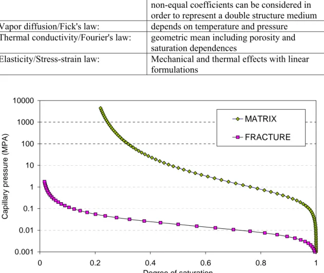
Figure 3.1-1. Retention curves for matrix and fractures.

Figure 3.1-1 shows representative retention curves that are considered by Birkholzer and Tsang (2000) for DST modelling. It can be observed that the matrix has a higher desaturation capillary pressure compared to the fractures, that desaturate at lower capillary pressures. Therefore, assuming equilibrium between fracture and matrix, desaturation in the rock will progress in the following way: first the fracture will desaturate and only when the fracture is practically desaturated (for instance at 0.1 MPa), the matrix is starting to desaturate.

The modified functions of relative permeability for the single structure analysis are shown in Figure 3.1-2 that consider m =0.04 for liquid and n = 0.8 for gas. It must be

noted that m = 0.04 is only considered for liquid relative permeabilities while the values of m for the retention curve of the matrix are maintained. In other words, the shape parameter is not the same in the retention curve and in the relative permeability functions because of the different importance of matrix and fracture. While matrix is important for storage of water, the fracture is important for the flow of water.

1.E-09 1.E-08 1.E-07 1.E-06 1.E-05 1.E-04 1.E-03 1.E-02 1.E-01 1.E+00 0 0.1 0.2 0.3 0.4 0.5 0.6 0.7 0.8 0.9 1 Degree of saturation Re lative per me ab ility kr,l: VG with m= 0.040 kr,g=Sg^0.8

Used in the

analysis (liq)

Used in the

analysis (gas)

Used in the

analysis (liq)

Used in the

analysis (gas)

1.E-06 1.E-04 1.E-02 1.E+00 1.E+02 1.E+04

Capillary pressure (MPa)

Per m eabili ty ( m 2)

MATRIX PERMEABILITY, krl with m= 0.247 FRACTURE PERMEABILITY, krl with m= 0.492 DOUBLE STRUCTURE MODEL

SINGLE STRUCTURE MODEL: krl with m=0.04 and Sl with m=0.247

Figure 3.1-2. Relative permeability functions used in single structure analysis (above) and equivalent permeability as a function of capillary pressure (below).

3.1.2.3 Equilibrium restrictions

Psychrometric Law and Henry’s Law are equilibrium restrictions. They give the partitioning coefficients for calculating the species mass present in each phase.

3.1.2.4 Additional hypothesis

The present analysis ignores the concrete invert at the base of the drift. The heat power is applied to the canister and the wings with a 70 % reduction of the actual value in order to consider, in an approximate manner, 3D thermal dissipation effects since the analysis is performed in 2D. This power reduction is a simplification of the actual situation. The adopted power values in canister and wings are:

Canisters: 36400W/canister/(9 canister x 4.7 m) = 860 W/m

Inner wing heaters: 37520 W/wings/(50 wings x 1.87 m) =401 W/m

Outer wing heaters: 55300 W/wings/(50 wings x 1.87 m) = 591 W/m

Figure 3.1-3 describe the power evolution in the time, a) canister and b) wings, according to experimental data, the line fit to actual power and the function considered. The application of a reduction of the power in the two-dimensional calculation is justified by thermal calculation of the three-dimensional problem (Appendix).

Liquid pressure at the bottom of the domain was calibrated in order to obtain a 92% degree of saturation in the initial phase taking into account the infiltration.

These parameters have been obtained from previously reported experimental data. Parameters are summarized in Table 3.1-2.

y = 130606e-0.0002167x 20 25 30 35 40 45 50 55 60 29 /07/1997 25 /01/1998 24 /07/1998 20 /01/1999 19 /07/1999 15 /01/2000 13 /07/2000 09 /01/2001 08 /07/2001 04 /01/2002 03 /07/2002 Date Can ister p o wer Actual power Function considered Fit to actual power

y = 1231707e-0.0002529x 30 50 70 90 110 130 150 170 29 /0 7/ 199 7 25 /0 1/ 199 8 24 /0 7/ 199 8 20 /0 1/ 199 9 19 /0 7/ 199 9 15 /0 1/ 200 0 13 /0 7/ 200 0 09 /0 1/ 200 1 08 /0 7/ 200 1 04 /0 1/ 200 2 03 /0 7/ 200 2 Date Wi ng h eaters p o w e r Actual Power Function considered Fit to actual power

Figure 3.1-3 Power in the different elements: in canisters (above) and in wings (below). The function considered corresponds to a fit for 2 years and 70% reduction.

Table 3.1-2 Parameters used in the modelling Mechanical

Elastic parameters

Young modulus, E 3.68E+04

Poisson coeff. ν 0.2

Thermal expansion coef. 2.00E-05

Thermal

Thermal conductivity

Dry 1.67

Saturated 2.10

Solid phase properties

Specific heat 865

Density 2510

Hydrological

Mat 3 Mat 2 Mat1

Porosity, 0.154 0.11 0.13 Retention curve Po (1/α) 0.0943 0.444 0.354 λ=m 0.243 0.247 0.207 Residual saturation 0.06 0.18 0.08 Maximum saturation 1 Molecular Diffusion

(

)

Exponential law: Variable with porosity k k= oexp

(

(

)

)

b = 500, 1000, 2000 and -1000

Liquid relative permeability: Van Genuch.

model, value of

λ

rg g e

3.1.3 Geometry, boundary conditions and mesh

We performed a two-dimensional (2-D) analysis on a rectangular model 180 m wide and 250 m high containing the 5 m diameter heated drift at the centre. The boundary conditions are shown in Figure 3.1-4. Initial conditions are obtained simply by calculating a steady state regime under isothermal conditions. This steady state was first obtained in a one-dimensional case. The negative water pressure imposed at the bottom boundary is selected in such a way that the initial degree of saturation in the vicinity of the drift is about 92%.

Figure 3.1-4. Geometry and boundary conditions for the THM problem.

This analysis has been performed with a mesh containing 2439 nodes and 4802 triangular elements, see Figure 3.1-5

T = 24º C Pg = 0.1 ql = 0 ux = 0 T = 24º C Pg = 0.1MPa Pl = -0.3 MPa uy = 0 T = 24º C Pg = 0.1 ql = 0 ux = 0 T = 24º C Pg = 0.1MPa ql = 0.36mm/year σy = 8 MPa x y 180

m

Figure 3.1-5. Finite element mesh used in THM calculations.

3.1.4. Results of temperature and water saturation

The distributions of temperature and degree of saturation after 90, 365 and 1460 days of heating are shown in Figure 3.1-7. It can be seen that the temperature distribution shows clearly the presence of the heaters. Degree of saturation is of the order of 0.92 at the level of the drift before heating started. Due to heating effects, drying takes place and degree of saturation decreases down to 0.25, which implies very high capillary pressures. After 365 days (1 year) of heating, the desaturated zone has a shape remarkably influenced by the wing heaters. After 1460 days (4 years) of heating, the desaturated zone is approximately elliptical.

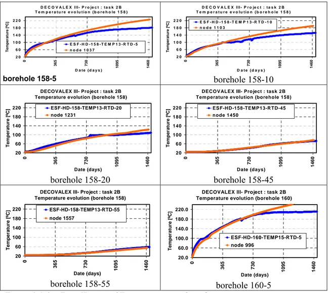
Figures 3.1-8 and 3.1-9 show the temperature evolution at different nodes, which are indicated in Figure 3.1-6. Comparison with measurements (which are included in each plot) indicates that temperatures are quite good in some points and show some deviations in others. Also, for the first two years results are better than for the third and fourth year.

Measurements were available for only two years when the TH modelisation was set up. For the first and second year, constant power (with only a slow decay) was considered appropriate. The constant power corresponds to 70% of the nominal value

(see Appendix). Power after two years would probably require a higher decay factor. This is confirmed by the too high temperatures calculated at some points for the 3rd and 4th _{year. However, since this is a 2D model, and uses a modified power, it was}

considered that further attempts to use a more realistic power were not justified.

Finally, profiles of temperature are represented in Figures 3.1-10 and 3.1-11 for boreholes 158, 160 and 162. The effect of the wing heaters is clearly observed in borehole 160 (this borehole is indicated in Figure 3.1-6). Profiles for the first and second year show good accuracy, but for longer times, temperature is overpredicted due to the reasons explained before.

As additional information, Figure 3.1-12 shows gas pressure development. It can be observed that the shape is similar, however, the gas pressures in the model calculations presented here are higher than the ones obtained by Datta (2002). This is probably due to the gas relative permeability curve which, in this simple porosity model, depends on the averaged gas saturation.

In order to understand completely the process of water flux, both in the liquid and in the gas phase according to this model, Figures 3.1-13 and 3.1-14 are included. Figure 3.1-13 shows liquid fluxes around the heated area. It can be observed that at one year the heating process is very active and water fluxes show the combined effects of drying and gravity. At four years, the dried zone is developing very slowly and diverts the vertical fluxes of liquid water due to its very low conductivity. Figure 3.1-14 shows that, for gas fluxes, gravity is not important due to the low density of gas. In fact, the gas phase is dominated by vapor and, hence, as the drying progresses these gas fluxes decrease near the heaters, but they are significant in the drying front. The drying front corresponds well with the elliptical shape observed in Figure 3.1-7.

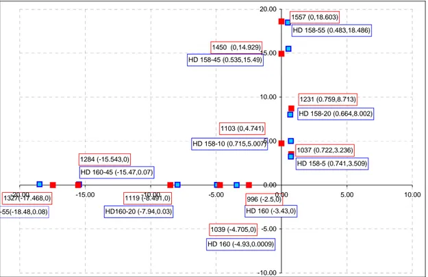
HD 160 (-3.43,0) HD 160 (-4.93,0.0009) HD160-20 (-7.94,0.03) HD 160-45 (-15.47,0.07) -55(-18.48,0.08) HD 158-5 (0.741,3.509) HD 158-10 (0.715,5.007) HD 158-20 (0.664,8.002) HD 158-45 (0.535,15.49) HD 158-55 (0.483,18.486) 996 (-2.5,0) 1039 (-4.705,0) 1119 (-8.491,0) 1284 (-15.543,0) 1327(-17.468,0) 1037 (0.722,3.236) 1103 (0,4.741) 1231 (0.759,8.713) 1450 (0,14.929) 1557 (0,18.603) -10.00 -5.00 0.00 5.00 10.00 15.00 20.00 -20.00 -15.00 -10.00 -5.00 0.00 5.00 10.00

Figure 3.1-6 Points with measurements and calculations of temperatures (x = 0 and y = 0 is the center of the drift). Note: This plot shows the actual location of the

measurement points in boreholes 158 and 160 and the corresponding nodes in the finite element mesh that were used for comparison.

Temperature distribution at

90 days. Degree of saturation distribution at 90 _days.

Temperature distribution at

365 days Degree of saturation distribution at 365 days.

Temperature distribution at

1460 days. Degree of saturation distribution at 1460 days.

Figure 3.1-7 Temperatures and degree of saturation distributions

3.1.5. Double Porosity Structure modeling by using CODE_BRIGHT

In the final phase of its Task 2 research the ENRESA team used a double porosity structure approach to perform THM modeling of the DST by the CODE_BRIGHT software. The TH aspect of this double structure modeling is described below.

3.1.5.1 Model description

The present model consists of a double structure approach to the problem of modelling the DST experiment at Yucca Mountain. The double structure approach is

D E C O V A L E X I I I- P r o je c t : t a s k 2 B T e m p e r a t u r e e v o l u t i o n ( b o r e h o l e 1 5 8 ) 2 0 6 0 1 0 0 1 4 0 1 8 0 2 2 0 0 365 730 _{1095 1460} D a t e ( d a y s ) T e mp eratu re [ ºC ] E S F - H D - 1 5 8 - T E M P 1 3 - R T D - 5 n o d e 1 0 3 7 borehole 158-5 D E C O V A L E X I I I - P r o je c t : t a s k 2 B T e m p e r a t u r e e v o l u t i o n ( b o r e h o l e 1 5 8 ) 2 0 6 0 1 0 0 1 4 0 1 8 0 2 2 0 0 365 730 _{1095 1460} D a t e ( d a y s ) Tem p er atu re [ ºC] E S F - H D - 1 5 8 - T E M P 1 3 - R T D - 1 0_{n o d e 1 1 0 3} borehole 158-10

DECOVALEX III- Project : task 2B Temperature evolution (borehole 158)

20 60 100 140 180 220 0 36 5 73 0 10 95 14 60 Date (days) Temperatu re [ ºC] ESF-HD-158-TEMP13-RTD-20 node 1231 borehole 158-20

DEC O VALEX III- Project : task 2B Tem perature evolution (borehole 158)

20 60 100 140 180 220 0 36 5 73 0 10 95 14 60 Date (days) Temperatu re [ ºC] ESF-HD-158-TEM P13-RTD-45 node 1450 borehole 158-45

DECOVALEX III- Project : task 2B Temperature evolution (borehole 158)

20 60 100 140 180 220 0 365 730 1095 1460 Date (days) T e mp er at ur e [ ºC] ESF-HD-158-TEMP13-RTD-55 node 1557 borehole 158-55

DECOVALEX III- Project : task 2B Temperature evolution (borehole 160)

20.0 60.0 100.0 140.0 180.0 220.0 0 36 5 73 0 10 95 14 60 Date (days) Te m p er a tur e [ ºC ] ESF-HD-160-TEMP15-RTD-5 node 996 borehole 160-5

Figure 3.1-8. Time History of Temperature at selected points DECOVALEX III- Project : task 2B

Temperature evolution (borehole 160)

20.0 60.0 100.0 140.0 180.0 220.0 0 36 5 73 0 109 5 146 0 Date (days) T e m p erature [ºC] ESF-HD-160-TEMP13-RTD-10 node 1039 borehole 160-10

DECOVALEX III- Project : task 2B Temperature evolution (borehole 160)

20.0 60.0 100.0 140.0 180.0 220.0 0 36 5 73 0 109 5 146 0 Date T e mperatu re [ ºC] ESF-HD-160-TEMP15-RTD-25 node 1119 borehole 160-25

D E C O V ALE X III- P roject : task 2B Tem perature evolution (b orehole 160)

20.0 60.0 100.0 140.0 180.0 220.0 0 365 730 1 095 1 460 D ate T e m p er at u re [ ºC ] E S F-H D -160-TE M P 15-R TD -45 node 1284 borehole 160-45 D E C O V AL E X III- P ro je c t : ta s k 2 B T e m p e ra tu re e vo lu tio n (b o re h o le 1 6 0 ) 2 0 .0 6 0 .0 1 0 0 .0 1 4 0 .0 1 8 0 .0 2 2 0 .0 0 365 730 1095 1460 D a te Tempe rature [º C] E S F -H D -1 6 0 -T E M P 1 5 -R T D -5 5 n o d e 1 3 2 7 borehole 160-55

DECOVALEX III-Project: task 2A borehole 158 (3 months) 20 40 60 80 100 120 140 160 180 200 220 240 0 4 8 12 16 20 distance [m] te mper at ure [º C ] 90 days exp. data borehole 158 at 90 days.

DECOVALEX III-Project: task 2A borehole 160 (3 months) 20 40 60 80 100 120 140 160 180 200 220 240 0 4 8 12 16 20 distance [m] te mper at ure [ ºC] 90 days exp. data borehole 160 at 90 days.

DECOVALEX III-Project: task 2A borehole 158 (1 year) 20 40 60 80 100 120 140 160 180 200 220 240 0 4 8 12 16 20 distance [m] te m p erat u re [ ºC ] 365 days exp. data borehole 158 at 365 days.

DECOVALEX III-Project: task 2A borehole 160 (1 year) 20 40 60 80 100 120 140 160 180 200 220 240 0 4 8 12 16 20 distance [m] te m p erat ur e [ ºC ] 365 days exp. data borehole 160 at 365 days.

DECOVALEX III-Project: task 2A borehole 158 (4 years) 20 40 60 80 100 120 140 160 180 200 220 240 0 4 8 12 16 20 distance [m] te mpe rat u re [ ºC ] 4 years exp.data borehole 158 at 1460 days.

DECOVALEX III-Project: task 2A borehole 160 (4 years) 20 40 60 80 100 120 140 160 180 200 220 240 0 4 8 12 16 20 distance [m] te m p er at u re [ ºC ] 1460 days exp. data borehole 160 at 1460 days.

DECOVALEX III-Project: task 2A borehole 162 (3 months) 20 40 60 80 100 120 140 160 180 200 220 240 0 4 8 12 16 20 distance [m] te m p erat u re [ ºC] 90 days exp. data borehole 162 at 90 days.

DECOVALEX III-Project: task 2A borehole 162 (1 year) 20 40 60 80 100 120 140 160 180 200 220 240 0 4 8 12 16 20 distance [m] te m p e rature [ ºC] 365 days exp. data borehole 162 at 365 days.

DECOVALEX III-Project: task 2A borehole 162 (4 year) 20 40 60 80 100 120 140 160 180 200 220 240 0 4 8 12 16 20 distance [m] tem p er a tu re [º C] 1460 days exp. data borehole 162 at 1460 days.

Figure 3.1-11. Profile of temperature at selected boreholes

0.09 0.1 0.11 0.12 0.13 0.14 0 10 20 30 40

long along Hole 76

Pg (M Pa ) 188.2 (180d=6months) 364.93 (365d=1year) 725.13(730d=2year) 1103 (1095d=3year) 1469.9 (1460d=4year)

Liquid fluxes for 1 year. Gas fluxes for 1 year

Liquid fluxes for 2 years. Gas fluxes for 2 years

Liquid fluxes for 4 years. Gas fluxes for 4 years

Figure 3.1-13 Liquid fluxes for 1, 2

and 4 years. All flux vectors are

represented with the same scale.

Figure 3.1-14 Gas fluxes for 1, 2 and 4 years. All flux vectors are represented

achieved by means of a two meshes that are connected with one dimensional elements. Among other aspects, the present analysis takes into account the concrete invert at the base of the drift, which was not included in the single structure analysis considered previously. The heat power is applied to the canister and the wings using a reduced power of 70% of the nominal value. This reduction permits to obtain reasonable temperatures in the 2D case, even though it can not be considered a general rule. In fact, three dimensional effects are not negligible in this case and a simple way to improve the predictions of a 2D calculation is using a reduced power. A comparison of a simple thermal calculation i.e. only with heat flow is performed in 2D and 3D and has been included in an appendix in order to demonstrate the convenience of using a reduced power.

The model takes advantage of symmetry for the design of the mesh. Figure 3.1-15 shows a schematic representation of the way that the two meshes considered are connected. For each point in the domain, there is an element that belongs to the matrix and an element that belongs to the fracture. These elements are connected using 1-D elements between nodes of each medium. The length of the connexion between the matrix and fracture is a key parameter in the model. A reference value of the distance of connexion between the matrix and the fracture is 0.01 m (1cm).

As mentioned above, the concrete invert is taken into account, so there are eleven materials that can be seen in Figure 3.1-15. There are: 3 materials for the matrix, 3 materials for the fracture, 2 materials for the concrete invert, 1 material for the connexions and lineal elements that connect the heating nodes. This latter element is intended to get more homogeneous power distribution. The material parameters used in the modeling are summarized in Table 3.1-3.

The power applied to the heat sources is has been calculated on the basis of a 70% reduction from nominal power (see appendix). The actual heat power for the 2D model is calculated as:

•Canisters: 0.7x52000 W /(9 canister x 4.7 m) = 860 W/m •Inner wing heaters: 0.7x53600 W /(50 wings x 1.87 m) = 401 W/m •Outer wing heaters: 0.7x79000 W /(50 wings x 1.87 m) = 591 W/m

3.1.5.2 Domain considered and Finite Element mesh

The ENRESA team performed a two-dimensional (2-D) analysis on a rectangular model 180 m wide and 250 m high containing half of the 5 m diameter heated drift and the wings corresponding to the half of the drift considered. The mesh contains 4932 nodes and 12051 triangular elements, and can be seen in Figure 3.1-16.

3.1.5 Results obtained

The results corresponding to two calculations are presented in this section. The first calculation is characterized by very small diffusion of vapour since tortuosity coefficient was set to 0.05. This calculation only reached 2 years due to convergence problems related to the severe dry conditions occurring in the vicinity of the drift and wings. Since tortuosity coefficient was very small, vapour diffusion was also reduced and this case was referred as ND (No Diffusion) by comparison to another case that is described below which will be referred as MD (Maximum Diffusion). The MD case will incorporate a tortuosity coefficient equal to unity plus an enhancement factor in order to

increase the diffusivity in the low gas saturation zones. Firstly the results for the ND case are described. Afterwards, the MD case is explained and compared with the ND case.

u

= u

T

_{≠ T}

P

_{≠ P}

P

_{≠ P}

u

= u

T

_{≠ T}

P

_{≠ P}

P

_{≠ P}

m1 Matrix (estrat. Lower) m2 Matrix (estrat. Middle) m3 Matrix(estrat. Upper) m4 Concrete

m5 Fracture (estrat. Lower) m6 Fracture (estrat. Middle) m7 Fracture (estrat. Upper) m8 Concrete

m9 Connexion between matrix and fracture Figure 3.1-15. Schematic representation of the double structure approach

Figure 3.1-16. Finite element mesh used in THM calculations.

Table 3.1-3 Parameters for the different materials and constitutive laws.

Materials

Matrix Fracture Concrete invert Connexion

Properties m1 m2 m3 m5 m6 m7 m4 m8 m9 Elasticity 0.368×105 _0.368×105 _0.368×105 _0.368×106 _{- 0} Mechanical Poisson Mod. 0.2 0.2 0.2 0.2 - - Termal Coef. of thermal expansion 0.2×10 -04 _0.2×10-04 _0.2×10-04 _0.2×10-04 _{- -} Press a tem. 0.354 0.444 0.0943 0.0602 0.01027 0.006369 0.444 0.01027 0.1 Lambda 0.207 0.247 0.243 0.492 0.492 0.492 0.247 0.492 0.2 Residual 0.08 0.18 0.06 0.01 0.01 0.01 0.18 0.01 0.08 Retention curve Max. Saturac. 1 1 1 1 1 1 1 1 1 Constant 1 1 1 1 1 1 1 1 Relative meability to gas: krg Power 3 3 3 3 3 3 3 2.28 1-krl

Idem to liq.: krl Lambda 0.207 0.247 0.243 0.492 0.492 0.492 0.247 0.492 0.2 kxx (m2) 0.247×10-15 0.124×10-16 0.525×10-17 0.187×10-11 0.100×10-12 0.635×10-12 0.124×10-16 0.10×10-12 kyy (m2) 0.247×10-15 0.124×10-16 0.525×10-17 0.187×10-11 0.100×10-12 0.635×10-12 0.124×10-16 0.10×10-12 kzz (m2) - - - - - - 1×10-15 Intrinsic permeability Porosity 0.13 0.11 0.154 0.00329 0.00263 0.00171 0.11 0.00263 ≅0 Dry 1.59 1.67 1.15 0 0 0 3.00 0 1.59 Termal Conductiv. Wet 2.29 2.10 1.70 0 0 0 3.00 0 Specific heat 865 865 865 - - - 865 - - Density 2540 2530 2510 - - - 2530 - -

id. Phase prop.

Therm. Exp. _0.2×10-04 _0.2×10-04 _0.2×10-04 _{- - - 0.2×10}-04 _-

Sol Long. 0.3 0.3 0.3 0.3 0.3 0.3 0.3 10

Sol . Transv. 0.03 0.03 0.03 0.03 0.03 0.03 0.03 1

Heat long. 0.3 0.3 0.3 0.3 0.3 0.3 0.3 10

Dispersion de mass and energy

Heat transv. 0.03 0.03 0.03 0.03 0.03 0.03 0.03 1

Trotuosity 0.05 0.05 0.05 0.05

3.1.5.1 Results for ND case

The distributions of temperature in the matrix after 1 year and 2 years are shown in Figure 3.1-17, degree of saturation after 1 and 2 years of heating for the matrix and the fracture are shown in Figures 3.1-18 and 3.1-19 respectively. As indicated, this analysis reached two years of heating, and Figure 3.1-20 shows several hydraulic variables at the end of this period. It can be seen, that due to the high vapour concentration and almost fully dry conditions, some instabilities appeared in some nodes.

Degree of saturation in the matrix and fracture are completely different due to the different retention curve in the matrix and in the fracture. The effect of gravity is clearly observed, especially for the fracture which shows a downward water flow.

Figure 3.1-21 shows other variables, such as the mechanical ones at 2 years of heating, that is displacements, horizontal stress, vertical stress and shear stress. Mechanical problem is considered elastic only and permeability is considered constant in this analysis.

The temperature evolution is shown in Figure 3.1-22, liquid pressure evolution in the matrix is shown in Figure 3.1-23, and finally, vapour pressure evolution in matrix is shown in Figure 3.1-24. It can be seen that an attempt to reduce the power in order to avoid higher temperatures is considered but the problems still persisted. The vapour pressure above the atmospheric pressure is an indication that the results are not

sufficiently good and that convergence problems appeared due to insufficient vapour migration. Degree of saturation is of the order of 0.92 at the level of the drift before the heating starts. Due to heating effects, drying takes places and degree of saturation

Figure 3.1-17. Temperature distribution at 1 year (left) and 2 years (right) of heating in matrix

Figure 3.1-18. Degree of saturation distribution at 1 year of heating. Matrix on the left and fracture on the right

Figure 3.1-19. Degree of saturation distribution at 2 years of heating. Matrix on the left and fracture on the right

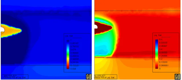
Figure 3.1-20. Hydraulic variables at 2 years. Liquid pressure (above left), gas pressure (above right), vapour mass fraction (below left) and liquid saturation (below right).

Figure 3.1-21 Mechanical variables at 2 years. Displacements (above left), horizontal stresses (above right), vertical stress (below left) and shear stress (below right)

20 40 60 80 100 120 140 160 180 200 0 365 730 1095 1460 Time (d) T (º C ) 3733 x= 2.5 y= 0.00 3417 x= 4.5 y= 0.00 2871 x= 8.72 y= 0.00 2373 x=15.02 y= 0.00 2175 x=18.58 y= 0.00 4227 x= 0.00 y= 2.95 4345 x= 0.00 y= 4.66 4483 x= 0.00 y= 9.03 4621 x= 0.00 y=15.12 4665 x= 0.00 y=18.02

Figure 3.1-22. Evolution of temperature in matrix.

-300 -260 -220 -180 -140 -100 -60 -20 20 0 365 730 1095 1460 Time (d) Li q u id pre s su re (MP a ) 3733 x= 2.5 y= 0.00 3417 x= 4.5 y= 0.00 2871 x= 8.72 y= 0.00 2373 x=15.02 y= 0.00 2175 x=18.58 y= 0.00 4227 x= 0.00 y= 2.95 4345 x= 0.00 y= 4.66 4483 x= 0.00 y= 9.03 4621 x= 0.00 y=15.12 4665 x= 0.00 y=18.02

Figure 3.1-23 Liquid pressure evolution in matrix

Matrix 0 0.05 0.1 0.15 0.2 0.25 0 365 730 1095 1460 Time (d) Vap our pres s u re (MPa) 3733 x= 2.5 y= 0.00 3417 x= 4.5 y= 0.00 2871 x= 8.72 y= 0.00 2373 x=15.02 y= 0.00 2175 x=18.58 y= 0.00 4227 x= 0.00 y= 2.95 4345 x= 0.00 y= 4.66 4483 x= 0.00 y= 9.03 4621 x= 0.00 y=15.12 4665 x= 0.00 y=18.02

decreases up to 0.25, which implies very high capillary pressures. These high capillary pressures are responsible, via psychrometric law, of maintaining the vapour pressure at atmospheric pressure. Otherwise, the vapor pressure at temperatures higher than 100oC is higher than atmospheric. The use of psychrometric law is not clear when the medium has been dried up strongly, with a sharp heating and capillary pressure increasing (liquid pressure decreases) up to values above 100 MPa, that are questionable. This probably requires a change in the state variable (for instance relative humidity or degree of saturation instead of liquid pressure).

3.1.5.2 Results for ND and MD cases

Since vapour mass fraction seems to reach a maximum value in the dry zone, it is possible that the diffusion of vapor play an importan role in this problem. It is clear that vapor flows by advection and by diffusion/dispersion. Advection is very efficient due to the high permeability of the fractures. However, diffusion of vapor is also a very efficient transport term due to the high diffussivity of vapour in air. Therefore a second case that considers very efficient diffusion is further considered.

Vapour diffusion enhancement is considered. An enhancement coefficient, is taken into account in the vapour diffusion law:

( ) ( )

ρ

ω

φ

τϖ

( )

φ

The enhancement factor can be explained by different processes. For instance, the meniscus are short-cuts, or the temperature gradients are locally higher than the ones that are used in the averaged approach. The enhancement factor equal to 1/Sg permits

enhanced vapor diffusion in high saturation zones, and the vapor mass fraction gradients are less pronounced. A vapor diffusion more efficient implies that the liquid pressure decreases more rapidly because the vapor pressure is controlled by liquid pressure through psychrometric law.

The case that has been described above is referred here as ND (No Diffusion) because molecular diffusion of vapor was very low (tortuosity coefficient equal to 0.05). In contrast the new case is referred as MD (Maximum Diffusion) because the tortusity is set to 1 and the enhancement factor has been included. A new FE mesh has been considered for the MD case with 6508 nodes and 15973 elements. Figure 3.1-25 shows this mesh and the zoom of centre part.

Figures 3.1-26 and 3.1-27 show a comparison between the two cases ND (already described above) and MD for degree of saturation in matrix and fracture at 1 year heating, respectively, and figures 3.1-28, 3.1-29 show the also degree of saturation but for 2 years of heating. From these plots, it can be seen that the dried zone is rather similar, but somewhat larger in the MD case. In contrast, the wetted zone, especially below the drift shows more development in the ND case than in the MD case. For the fracture, the maximum saturation reaches 0.6 while for the MD it hardly reaches 0.3. This wetted zone extends downwards for the ND case reaching practically the lower formation while in the MD case it is much smaller.

Matrix Fracture

Figure 3.1-25. Finite element mesh used for the MD case

Figure 3.1-26. Matrix degree of saturation at 1 year. ND case on the left and MD case on the right

Figure 3.1-27. Fracture degree of saturation at 1 year, ND case on the left and MD

Figure 3.1-28. Matrix degree of saturation at 2 year. ND case on the left and MD case on the right.

Figure 3.1-29.Fracture degree of saturation at 2 years. ND case on the left and MD case on the right.

3.1.5.3 Results for MD case at 4 years

Figure 3.1-30 shows for the MD case that at 4 years, the development of the wetted zone below the canister is larger and comparable to the one obtained for 1 or 2 years for the case ND.

Figures 3.1-31 and 3.1-32 show liquid and gas fluxes in the matrix and in the fracture for the MD case. It can be seen that liquid fluxes are important in both, matrix and fracture, while gas fluxes are only important for the fracture. Liquid flow is not important in the dried zone. Gas flow towards the drift and towards the heaters ins motivated by the boundary condition of constant gas pressure in these boundaries.

Figures 3.1-33, 3.1-34, 3.1-35, 3.1-36, 3.1-37, and 3.1-38 show respectively the temperature, liquid pressure, vapour pressure, vapour mass fraction, degree of saturation for matrix and degree of saturation for fracture. Temperature evolution shows the effect of evaporation in points that are heated slowly. Liquid pressure shows that drying implies a large decrease to negative values with low physical meaning, except that this liquid pressure, once introduced in psychrometric law gives a relative humidity that is used for calculation of vapour pressure and vapour mass fraction. The physical meaning

is recovered. Therefore, such low liquid pressures may be considered only intermediate variables and impossible to measure directly.

It can be seen that vapour pressure is much more realistic (reaches atmospheric pressure but not much higher and remain more stable) for the MD analysis (Figure 3.1-35) than for the ND analysis (Figure 3.1-24).

Only for degree of saturation it is relevant to differentiate the matrix and the fracture. It is relevant to see the evolution of degree of saturation in points that undergo wetting and in points that undergo drying. After the drying front passes, degree of saturation in the matrix tends to a value in the range of 0.2 to 0.3 while the fracture reaches values practically zero. From these plots, it can be stated that steady state regime is not reached.

Figure 3.1-30.Matrix and Fracture degree of saturation at 4 years for case MD.

Figure 3.1-32.Matrix and Fracture gas fluxes at 4 years for case MD 20 40 60 80 100 120 140 160 180 200 220 240 260 0 365 730 1095 1460 Time (d) T ( ºC ) 2446 x= 2.5 y= 0.00 2310 x= 4.6 y= 0.00 2014 x= 8.8 y= 0.00 1618 x=14.3 y= 0.00 1438 x=18.2 y= 0.00 2711 x= 0.00 y= 2.9 2803 x= 0.00 y= 4.6 2979 x= 0.00 y= 8.9 3093 x= 0.00 y=14.0 3125 x= 0.00 y=18.5

Figure 3.1-33.Temperature evolution at different points for case MD

-800 -700 -600 -500 -400 -300 -200 -100 0 100 0 365 730 1095 1460 Time (d) Li q u id pr es sur e ( M Pa) 2446 x= 2.5 y= 0.00 2310 x= 4.6 y= 0.00 2014 x= 8.8 y= 0.00 1618 x=14.3 y= 0.00 1438 x=18.2 y= 0.00 2711 x= 0.00 y= 2.9 2803 x= 0.00 y= 4.6 2979 x= 0.00 y= 8.9 3093 x= 0.00 y=14.0 3125 x= 0.00 y=18.5

0.00 0.02 0.04 0.06 0.08 0.10 0.12 0.14 0.16 0.18 0.20 0 365 730 1095 1460 Time (d) Vapour pres s u re 2446 x= 2.5 y= 0.00 2310 x= 4.6 y= 0.00 2014 x= 8.8 y= 0.00 1618 x=14.3 y= 0.00 1438 x=18.2 y= 0.00 2711 x= 0.00 y= 2.9 2803 x= 0.00 y= 4.6 2979 x= 0.00 y= 8.9 3093 x= 0.00 y=14.0 3125 x= 0.00 y=18.5

Figure 3.1-35.Mass fraction of vapour for the case MD

0 0.1 0.2 0.3 0.4 0.5 0.6 0.7 0.8 0.9 1 0 365 730 1095 1460 Time (d) Vapo ur m a s s f ract ion _{2446 x= 2.5 y= 0.00 2310 x= 4.6 y= 0.00} 2014 x= 8.8 y= 0.00 1618 x=14.3 y= 0.00 1438 x=18.2 y= 0.00 2711 x= 0.00 y= 2.9 2803 x= 0.00 y= 4.6 2979 x= 0.00 y= 8.9 3093 x= 0.00 y=14.0 3125 x= 0.00 y=18.5

Figure 3.1-36.Mass fraction of vapour for the case MD

Matrix 0.00 0.10 0.20 0.30 0.40 0.50 0.60 0.70 0.80 0.90 1.00 0 365 730 1095 1460 Time (d) De gr ee of s a tu ra tion 4627 x= 2.5 y= 0.00 4643 x= 4.6 y= 0.00 4721 x= 8.8 y= 0.00 4761 x=14.3 y= 0.00 3363 x=18.2 y= 0.00 4847 x= 0.00 y= 2.9 5349 x= 0.00 y= 4.6 7711 x= 0.00 y= 8.9 2271 x= 0.00 y=14.0 2297 x= 0.00 y=18.5

Fracture 0.00 0.10 0.20 0.30 0.40 0.50 0.60 0.70 0.80 0.90 1.00 0 365 730 1095 1460 Time (d) D egr ee of s a tu ra tion 4628 x= 2.5 y= 0.00 4644 x= 4.6 y= 0.00 4722 x= 8.8 y= 0.00 4762 x=14.3 y= 0.00 3364 x=18.2 y= 0.00 4848 x= 0.00 y= 2.9 5350 x= 0.00 y= 4.6 7712 x= 0.00 y= 8.9 2272 x= 0.00 y=14.0 2298 x= 0.00 y=18.5

Figure 3.1-38.Fracture degree of saturation for the case MD

3.1.5.4. Conclusions

The analyses presented here are the firtst attempt to use a finite element double structure approach to solve the THM problem simulating the DST test at Yucca Mountain. In this model, symmetry has been incorporated to allow mesh refinement. With this model the double structure formulation has been validated.

The tortuosity and enhancement coefficients are key parameters and vapour diffusion plays an important role as shown by the calculations. Liquid pressure controls vapour concentration via psychrometric law, vapour concentration tends to 1 in the dry zone, therefore air tends to disappear. Gas pressure gradients are not sufficient to dissipate vapour concentration if vapour diffusion is small.

On the other hand, liquid flow is driven by gravity, but this effect is more evident when vapour diffusion is smaller. Also the phase change signature is more evident when vapour diffusion is small.

3.2 NRC research team’s TH modeling

The NRC research team’s TH modeling of the DST for DECOVALEX III Task 2A is documented in this Section 3.2. The NRC team’s initial predictive modeling was described in the Task 2A Interim Report prepared in February 2002. The NRC team later performed further refined modeling including comparative analyses with measurements and submitted its contribution for the Task 2A Final report in October 2002. This Section 3.2 of the present Task 2A Final Report is a composite, subsuming the NRC team’s TH modeling and analyses relevant to Task 2A of DECOVALEX III project.

3.2.1 Introduction

The NRC research team modeled the thermal-hydrologic (TH) response of the DST employing the numerical modeling code MULTIFLO (Lichtner et al 2000). MULTIFLO is a general purpose code for modeling mass and energy transport processes in multiphase, non-isothermal systems with chemical reactions and reversible and irreversible phase changes in solids, liquids, and gases. The code consists of two sequentially coupled sub-modules: Mass and Energy Transport (METRA) and General Electromagnetic Migration (GEM). Only the transport of air, water, and heat in the DST was simulated for the Task 2A exercise using the METRA sub-module and reported in the Task 2A Interim report of February 2002. For subsequent refinement modeling MULTIFLO Version 1.5.1 (Painter et al 2001) was used to perform the simulations. Conceptual models for dual continua and the active fracture model (Liu, et al., 1998) were also evaluated. Temperatures measured during the 4-year heating phase of the Drift-Scale Heater Test were used as the basis for the evaluations.

3.2.2 Mathematical

setting

In the MULTIFLO code METRA solves mass balance equations for water and air and an energy balance equation. Additional descriptions of flux terms between the matrix and fracture continua and of the active fracture model have been added here because of their importance in the analysis of the DST.

METRA represents multiphase flow through three dimensions, although zero, one, or two dimensions are also possible. Single-phase (i.e., all liquid or all gas) or two-phase systems can be simulated. The equation of state for water in METRA allows temperatures in the 1to 800°C range and pressures below 165 bars. A description of the mathematical basis for METRA is presented below. A discussion of the balance equations is followed by the constitutive equations and the dual continuum model formulation.

3.2.2.1 Conservation equations

The conservation equation for the water component (w) is given by

(

)

[

]

(

)

(

)

[

]

(

)

∂

∂

ϕ

ϕ

Subscripts and superscripts g and l denote the gas and liquid phases. In these equations,

mass transport, ql and qg, is represented by Darcy’s Law (as modified by the relative

permeability for multiphase flow), which includes capillarity, gravity, and viscous forces