Forecasting of ExchangeRate: Autoregressive modelsvs. XGBoost

BACHELOR THESIS WITHIN: Economics NUMBER OF CREDITS: 15ECTS

PROGRAMME OF STUDY:International Economics

AUTHOR: Hinda Ahmed, Moaz Alhomsi JÖNKÖPING Month Year-December 2020

Forecasting of Exchange

Rate: Autoregressive models

vs. XGBoost

Bachelor Thesis in Economics

Title: Forecasting of Exchange Rate: Autoregressive models vs. XGBoost Authors: Hinda Ahmed, and Moaz Alhomsi

Tutor: Andrea Schneider Date: 2020-12-07

Key terms: Exchange rate, Machine Learning, Forecast, Out-of-Sample, XGBoost, ARDL, Random walk, Decision tree

Abstract

In international economics and trading, the exchange rate is important. Forecasting the exchange rate helps in minimizing risks and maximizing profits. The study attempts to test three models to forecast EUR/USD exchange rate. Based on previous work by Meese & Rogoff (1983), we replicated the authors work of the Random Walk model of AR(1) on different period and currency to check if the model was able to forecast the exchange rate. Then we ran ARDL and XGBoost models to find which of the two models performed better than the Random Walk model based on different measures. The measures are Root Mean Square Error (RMSE) and Direction Accuracy. First difference was taken to remove unit root from ARDL and XGBoost models. Adding lags to the independent variables in addition to the dependent, AR(1), generated better outcome. This is an indication of how variables take different periods to affect the dependent variable. Moreover, choosing leading indicators like economic policy uncertainty index and Euro futures helped the model in forecasting. The result showed that ARDL and XGBoost models were able to forecast two periods prior the event took place, while the Random Walk model was not able to forecast rather it replicated the previous period, i.e., it was lagging.

Table of Contents

1 Introduction ... 1

2 Literature review ... 3

3 Background ... 5

4 Theoretical background ... 6

5 Data ... 7

6 Empirical study ... 8

6.1.2.1 Random Walk model ... 13

6.1.2.2 ARDL model ... 15 6.2 Machine Learning ... 18 6.3 Comparison of models ... 23

7 Conclusion ... 26

References ... 27

Figures

Figure 4.1 Conceptual framework ... 6

Figure 6.1 The Actual is the exchange rate through the interval 2018-2020 and the predicted is its prediction. ... 11

Figure 6.2 The series (EURUSD) and its forecast (EURUSDF) of its first lag... 13

Figure 6.3 The Actual (EURUSD) and a lag of its forecast. ... 14

Figure 6.4 First difference of the series Exchange Rate (DEURUSD) and its forecast ... 16

Figure 6.5 XGBoost way of using more than a tree for estimation. ... 22

Figure 6.6 XGBoost - The Actual is the exchange rate through the interval 2018-2020 and the predicted is its prediction. ... 22

Figure 6.7 XGBoost - First difference of the series Exchange Rate (DEURUSD) and its forecast ... 23

Figure 6.8 Prediction of models in previous crisis………. 26

Tables

Table 6.2 Output Random Walk AR(1) ... 12

Table 6.3 Output of ARDL Model ... 17

Table 6.4 Measurements of the models ... 24

Table 6.5 Forecast and Actual Granger Causality in Random Walk model ... 24

Table 6.6 Forecast and Actual Granger Causality in ARDL model ... 24

Table 6.7 Measurement of previous crisis prediction ... 25

Appendix

Appendix B ... 34

1. Introduction

Exchange rate is crucial in international economics and trade, predicting the exchange benefits investment funds like hedge funds in risk elimination. It also benefits the federal institutions like the Euro commission and Federal Trade Commission in making decisions about trading and new legislation. Forex, also known as foreign exchange (FX), is a the most liquid market which is the largest currency trading in the world. Currencies around the world are bought or sold by paring the two currencies making it very vital in the topic of economics. As mentioned in Kumar (2014) this market of currency has different participants being investors, central banks, hedge funds, and commercial banks. The main purpose of this liquid market is for the stability of the financial institution that plays a role in the inflation control of a country. King et al. (2011, p11) mentioned that ``Since financial institutions use currencies primary as a store of value, they gain or lose according to future changes in the currency’s value ``. Investment is an important factor in an economy and with the help of Forex market, investors create market overseas for their products and services, build strategic asset and expand their firms abroad and find cheaper source of production and service for their market, in addition to investment, investors will always seek a way to protect their investments by hedging (Connor & Woo 2004).

Hedging is a process by which an investor can secure their capital or investments, in worst case scenario as a risk management tool and not lose a lot of money because of fluctuation for a business transaction that took place which might result in a loss in interest (Stulz ,1996). Through hedging, investors can prevent losses in transaction, payments and receipts could also be secured. Among the factors that affect the Forex market are also the inflation rate and interest rates that are inversely related. When the interest rates are increased, it causes currency appreciation. The theories in economy confirms that in a free/floating currency, the value of money always change regarding the demand and supply in the forex market. interest rates can be influenced by a factor like the monetary policy by the central bank which uses this as a control mechanism to defend the local currency. this can either be by raising or lowering the interest rate. Higher interest rates attract investors and therefore currency appreciates. The opposite effect is that a lower

interest rate discourages investors and therefore currency deprecation. Several more factors can affect the exchange rate, depending on what type of currency we are analyzing. Is it a pegged currency like the Gulf Cooperation Council countries (G.C.C) currencies except Kuwait? Is it a commodity backed currency like the Australian dollar and the Canadian dollar? Which regime is it following a floating or fixed?

In our paper, we focus on two free floating currencies, the Euro/US dollar (EURUSD). We believe that this thesis can contribute a lot because for every economy, the norm is fluctuation since the currencies are floating exchange rates. We try to bridge into a way of understanding the relationship between the complex forex market and the prediction needed for the future of the currency value. This will benefit the stakeholders of the Forex market in general mostly investors. For this paper, we will compare two models. The first is autoregressive distributed lag (ARDL) which is the integration of autoregressive model and the distributed lag. The second is the Machine learning model-based algorithm called the XGBoost. Separately, both models are tested and compared to see which one can forecast better in comparison to the Random Walk model, as Meese & Rogoff (1983) argued that no exchange rate model can outperform the Random Walk model. The data is mainly retrieved from St. Louis feds and European commission. In addition, we got Euro FX futures of non-commercial (money institutions) from the Commitment of Traders report of futures only and Economic Policy Uncertainty Index. The sample size for this study will be 215 for the fundamental model, 212 for the ARDL and 215 for the Random walk model. Monthly data are used from 2000 to 2020. For this study we will do as follows:

1. Use fundamentals with no lags, where factors are taken based on economics theory. To base it on economic theory and build the following models accordingly.

2. Use only a lag of the dependent variable (random walk), a lag of the dependent variable is the previous period. Then we will be taking the difference of variables, used in the fundamental model to become stationary and add lags to the independent variables, where it becomes ARDL model.

3. Same as the ARDL model but it will be run in XGBoost, a machine learning model based on decision tree approach.

The out-side-sampling is used in this paper, which means that the trained data and a test data are separate. When the data is trained on data set, the test set will be different from that of trained set. The error of forecasting that occurs is calculated from the test set. Forecasting and prediction are not used interchangeably in this paper. Prediction will be used in the fundamental model because it lacks lags, which means that it will not generate prognostic data. while forecasting will be used in Random-walk and ARDL models, on the grounds of lags that are used in these models to prognose. In addition, XGBoost will be used as both predictive and forecasting model.

This thesis has 6 sections. The first part being the introduction, the second is the literature review as foundation to our study with mentioning previous researchers and their findings. We look into different schools of thoughts regarding forecasting exchange rates. In the third section we have the theoretical background where we discuss theories that affect the dependent variable in relation to the independent variables. in the fourth section, we will explain the variables that we chose and define them. The Empirical part is the fifth section, results and approaches will be explained. The sixth section is the last, we will conclude this study and add limitations and suggestions for future studies and recommendations.

2. Literature Review

This paper focuses on the models that predict the foreign exchange market. There are a lot of studies and prediction models that have evolved over the years. Meese and Rogoff (1983) are possibly the most often cited study regarding forecasting exchange rate. How well can macro models perform in forecasting the exchange rate is a question of a lot of researchers. It was after the fall of the Bretton woods system that certain forecasting models were introduced. It suggested that macroeconomic variables affect the exchange rate. It is against this theory that Meese and Rogoff (1983) argued against in their paper. The original work of these two authors indicated that random walk models, with or without a drift model, can do more predicting than macro models.

For around 40 years ago Meese and Rogoff (1983) argued that a random walk model can predict the exchange rate better than other models. Back in 1983 a lot of measures were

not yet discovered or used. In addition, not enough data was available back then, especially post- Bretton Woods system, where exchange rates became floating after being fixed regimes. Moreover, the main problem in their study is that the lag of the dependent variable, which is the independent variable in the random walk model, is technically predicted by the dependent variable and not vice-versa where the main topic is predicting the exchange rate by its lag and not the way opposite. In Demystifying The Meese-Rogoff Puzzle, Moosa and Burns (2015) argued that in addition to the problem mentioned above, Meese and Rogoff (1983) used measurement of magnitude, Root Mean Squared Error, only without considering a direction measurement, but what is actually the case in the latter problem is that using a magnitude measurement was helpful but being the only measurement used was inaccurate. The out-side-sampling is used in this paper, where the forecasted sample is not in the studied sample or in a trained dataset for the XGBoost model. The outcome we got is that the random walk model forecasted the worst, but the ARDL models performed better.

Looking back to the previous researchers, In the early 20th century, economists, mathematicians and statisticians came together in developing models and forecasts that have contributed much to recent studies. From the 1930s onward Keynesian macroeconomics became very popular. Diebold, F. X. (1998) suggested that in the book published 1936 The General Theory of Employment, Interest, and Money considered that market being unstable fundamentally and suggested the government as stabilizer. This book introduced the hybrid model of statistics and economic theories for the forecasting macro variables. By the 1970s, Keynesian theories started showing that these factors that were unexplained in his theories like the rate of the interest and monetary natures that were important variables to the economy and prediction of the future exchange rate were not considered important or was not explained well how they fit in an economy.

Mark (1995) argued that if the statistics were used more than the monetary fundamentals like money supplies, interest rates and output, it will explain the behavior of the exchange market. Cheung et al. (2005) mentioned that adding improvement on the models of the 1970s like the purchasing power parity (PPP) or real interest differentiation model will give us a better result as in the forecasting exchange rate. The purchasing power parity (PPP) model as a forecasting method theory suggests that the exchange rate will adjust

by counterweighting the price change that happens due to inflation. This means a constant equilibrium level to exchange rate which means that the foreign currency should have the same purchasing power. This theory contradicts Meese and Rogoff that suggested that countries that have almost similar inflation, cannot have economic fundamentals like money supply, income, trade balance and other variables as a forecasting exchange rate between counties. Mees and Rogoff mentioned in their paper that factors that have impact on exchange rates are national money supplies, real incomes, short-term interest rates, expected inflation differentials, and cumulated trade balances. Studies that were done after the 1983 paper is mostly based on the importance of the variables that are mentioned as determinants of exchange rate. Muusa (1985), Frankel and Rose (1995), Evans and Lyons (2002), Cheung (2002) and Nahid, (2007) are some of the authors supporting that random walk can predict more than any macro model. On the contrary we have authors that say that the fundamentals are still very crucial determinants in exchange rate. Authors like Brooks (2001), Kilian and Taylor (2001), Menzie et al. (2006) and Taylor and peel (2000) are some authors that suggest that random walk performs very poorly in prediction for the foreign currency.

3. Background

How did the Foreign exchange market (FOREX) get started? First, gold was the commodity that served as exchange for goods. But it became devaluated after the second world war with so many countries being in debt and printing money and not having enough gold to substitute. The Bretton Woods system (1944/1971) was the beginning of the new order in the global economy (Ghizoni 2013). The United States, Britain and France met in Bretton Woods in the United nation monetary and finance conference. In order to avoid a monetary crisis, the exchange rate was made fixed with the US dollar as the primary currency reserve replacing the gold. This was done as the United states were the only country that did not suffer the war economically therefore superpower. The International Monetary Fund (IMF), world bank and the General Agreement on Trade and Tariffs (GATT) were formed as institutions to assist this market. According to

Truman (2017) the agreement was replaced 1971 by a different valuation currency system. The US currency was made free floating against other currencies which marks the beginning of the modern forex market.

4. Theoretical background

First, we will look into the exchange rate as a variable. The exchange rate market is the most liquid market with a pairing of the quotation with the value of one currency unit against another. The exchange rate regime can be pegged, floating, fixed or hybrid. Exchange rate as a variable, it is not constant which means it is determined by different factors like inflation, Gross Domestic Product (GDP), Balance of Payments (BOP), Money Supply (M2) and interest rates. In this paper we are going to choose two factors the money supply and balance of payments (Laurin and Martynenko ,2009).

According to Cornell (1982), money supply affects the exchange rate by a change in the interest rate. If the countries money supply surpasses money demand, it causes a devaluation of domestic currency. On the other hand, what will cause the devaluation of foreign currency is domestic demand for money exceeding supply, relatively.

The Balance of Payment (BOP) is accounting record for a recorded time of the transaction. This business operation includes export, import, financial capital, and transfers. It is summarized for specific time, mostly a year using a single domestic currency (Makin ,2002).

As in Figure 4.1, it gives an overview about how the models were structured. The independent variables on the left are directly affecting the dependent variable on the right.

5. Data

We used monthly data for the EURUSD exchange rate for the time period between years 2000-2020. Thus, our data set covers a time series of around 240 months. The time period also covers three crises being the Financial crisis of 2007, Euro crisis of 2009 and the Covid19 of 2020. The models were trained for the first two events and it will forecast the third event. We will see how the result show in the empirical analyses. Our main variable of interest is the exchange rate. In addition, five of the control variables are mentioned below. The majority of the data is provided by St. Louis feds and European commission.

1) Euro futures (EUROFX) are trading futures in short term interest rate which is

contracted under the list of the Chicago mercantile. The Euro futures are contracts traded in the United States, part of commodity futures trading commission (CFTC) that has been active and traded for more than 150 years. Futures contracts fall under “Traders in Financial Futures” reports. We took the difference between long and short of non-commercial traders, they are institutions like hedge funds, they usually trade in large to huge positions and thus have an effect on the market. EUROFX is a pre-determinant factor, having more long contracts than short contracts, in Chicago Mercantile, will stimulate the Euro to appreciate against the USD.

2) Balance of payments (BOP) is financial transitions that take place in defined period

such as annually or quarterly of a year. It is the inflow and outflow of a goods, service and capital between countries. When a country's BOP changes it causes fluctuation, which causes the local of foreign currency to change. (Obstfeld & Krugman ,2003). The balance of payment theory of exchange rate suggests that a deficit in BOP resulting in depreciation and vice-versa. A deficit resulting in demand exceeding the supply or of foreign currency. This means that they are positively related. The data BOP-DIFF was taken from ST. Louis fed for both the Euro Area and the United States, we took the difference between the two economies’ balance of payments. As shown in the figure A2 in appendix A, when the

3) Benchmark indexes (IND): STOXX 50 - S&P 500 Benchmark indexes that have been

established to include many securities that reflect some part of the overall market. Talking about these two stock indexes, both show the large caps in both economies. Stocks are bought and sold, the price alone is not an indicator, but exchange rates play a crucial role in trading positions. Like in exports, the cheaper a currency, relatively, the more it will export, in most cases. So, stocks are no different, the cheaper the currency, relatively, the higher the index, but it is not always the case because after the high demand for a currency it will appreciate, then the index price will fall again. Money supply will equate demand, then the cycle starts over.

4) Money Supply (M2) Obstfeld and Krugman mention that, as a monetary policy, the

central bank uses it to control inflation. For this paper, we will look into the monetary approach to exchange rate. This approach suggests that the rate of exchange depend on balancing the supply and demand for currency of the country. There is no direct link between supply of money and exchange rate but through interest rate, it can be seen that there is a negative relation between them. The other theory is purchasing power parity (PPP), which shows an increase in money supply causes depreciation which makes the interest rate depend on the money supply as per the expectation of the people changing.

5) Economic Policy Uncertainty (EPU) it is an indicator of uncertainty in news of

economic policy in the two economies, USA and Euro Area (EA). Ten newspapers from the US and 8 newspapers from the EA and UK. The component that is used in this index is economic policy uncertainty related news (Economic policy uncertainty index, 12th October).

6) Exchange rate (EURUSD) is the dependent variable/target. It shows relatively how

many US dollars are per Euro, taken on monthly average.

6. Empirical Study

In this part, we will take use of the autoregressive distributed lag (ARDL) and the XGBoost model to predict the exchange rate, and then compare which of the methods produce better measurements. In the analysis, the variables used are those mentioned in

the theoretical background. To optimize the performance of the machine learning model, we use a sample size of 212 of which 90% of the dataset for the training set and 10% which has a sample size of 24 for the validation set. In the ARDL model we used the model with the least Akaike Information Criterion (AIC), with the same split of data we used in the XGBoost model in order to forecast the Euro / US dollar spot exchange rate. The below indicators are used.

- RMSE: Root Mean Squared Error, which yield the estimated value of the error square between the estimator and the true value of the parameter. (Everitt et al.,2010). When the RMSE is low, it means that the model is more accurate in forecasting. The result is obtained by squaring the rate of the absolute forecast minus the actual forecast. The errors became larger since we take the squared figure as outcome.

𝑅𝑀𝑆𝐸 = √1

𝑛𝛴(𝑦 − 𝑦̂)

2

RMSE is a good complementary measure where it shows how close is the estimated/predicted/forecasted series to the actual series. According to Moosa & Burns (2015), it is an inappropriate to use it as an only measure in our analysis.

- Direction accuracy: A measure of accuracy of direction between real and forecasted or prediction value.

The direction accuracy measurement that we have made is simple. First, we take 𝑨𝒄𝒕𝒖𝒂𝒍 (𝒚_𝒕− 𝒚_𝒕−𝟏) and 𝑭𝒐𝒓𝒆𝒄𝒂𝒔𝒕𝒆𝒅 (𝒚_𝒕− 𝒚_𝒕−𝟏), if 𝒚_𝒕 > 𝒚_𝒕−𝟏 it will result

in 1 and 0 when 𝒚_𝒕 < 𝒚_𝒕−𝟏. Then we take the difference of the two columns, Actual

and Forecasted. If both were equal, we get 0.

𝐷𝐴 = ∑ 𝑐𝑜𝑢𝑛𝑡(0)𝑠

𝑛_𝑠 ∗ 100

DA is the direction accuracy, where count(0) is how many times did we get 0 in our sample, the “s” stands for sample, then we divide it by the number of the sample and finally multiply it by 100 to get the percentage of “0’s” in the sample. This will decide if both series are moving together and by what percentage. Although it shows if both series,

estimated/predicted/forecasted and actual, moves together, but it does not include the magnitude i.e. it does not measure the distance between both series. That is why RMSE is good to be used as a complementary measure.

6.1 Econometrics

This area comprises several models that uses timeseries, like fundamental model, ARDL and Random Walk model, to find a better performing model based on the indicators mentioned above.

6.1.1 Fundamental model

Starting with the fundamental model that uses fundamental variables which are variables that do not have any sort of transformations nor lags and are based on economic theory. We have those variables mentioned in the conceptual framework Figure 4.1.

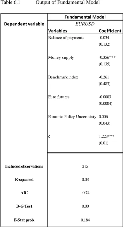
Statistically speaking, fundamental Model in Table 5.1 has an insignificant output, the F-Stat prob. Of 0.184 shows that up to 10% of significant level we may not reject the null hypothesis of F-Stat, we conclude that at least one variable, conjointly with other variables in a model, is not significant and does not affect the dependent variable. But this model is used as a fundamental model, i.e., model based on economic theory without adding lags. R-squared, the coefficient of determination, is low here, where it measures the variance in the dependent variable explained by the independent variable(s). Moreover, the Breusch-Godfrey test (B-G Test) shows a significant value of 0.00 where we may reject the null hypothesis of the B-G test which states no autocorrelation hence, we conclude that there is an autocorrelation in our model. Although only one variable is significant, the money supply. Some variables have a long run relation, i.e., take time to show an impact on the exchange rate (EURUSD). Like the case in future contracts (EUROFX), even the other variables have lagging values from the moment they are announced. Either we get higher frequency data that are premium data, needs a subscription, and more precise or use lags in our model.

(1)

The sub notation t indicates that the series is a timeseries, the 𝛽_𝑛 in 𝛽_𝑛𝑋_𝑛 is a coefficient, also called weight, which shows the change of one unit or percentage in x affecting y. 𝛽₀ indicates the y-intercept that shows if all coefficients were zero, the dependent variable, y, on average is equal to 𝛽0. ɛ𝑡 is an error term.

Table 6.1 Output of Fundamental Model

𝐸𝑈𝑅𝑈𝑆𝐷

= 𝛽

+ 𝛽

𝐵𝑂𝑃_𝐷𝐼𝐹𝐹

+ 𝛽

𝑀2_𝐷𝐼𝐹𝐹

+ 𝛽

𝐼𝑁𝐷_𝐷𝐼𝐹𝐹

+ 𝛽

𝐸𝑈𝑅𝐹𝑋

+ 𝛽

𝐸𝑃𝑈_𝐷𝐼𝐹𝐹

+ ɛ

(0.043) c 1.223*** (0.01) B-G Test Fundamental Model EURUSD Included observations R-squared AIC 215 0.03 -0.74 0.00 F-Stat prob. 0.184

Notes: The Asterisk stands for significance level (*** significant at 0,01 level , ** significant at 0,05 level and * significant at 0,1 level). Breusch-Godfrey serial Correlation LM test (B-G Test) result is the prob. of Chi-squared, F-Stat prob. Is the p-value of the F-Stat. DIFF stands for the difference between the variables in both economies USA and EA, except for EUROFX where DIFF stands for difference between long and short contracts.

Trying to predict the exchange rate with the variables in Table 6.1, with the fundamental model:

Fig 6.1 The Actual is the exchange rate through the interval 2018-2020 and the predicted is its prediction.

6.1.2 Autoregressive Models

Most forecasting problems involve the use of time series data. `` A time series is a time-oriented or chronological sequence of observations on a variable of interest. `` (Montgomery et al. 2015, p2). Observing and predicting in econometrics is done by time series which is data collected in different points in time. Analyzing the data due to its past nature gives us the prediction needed regarding economic forecasting in the future. Lagged variables are used to refer to the prior time in correlation to the current time. Factors that affect the times series are trends, cyclical, seasonal and irregular. By nature, this model is stochastic which means that certainty is quite low. On the other hand, it is stationary since the mean, covariance and variance do not change over time. We will go through two types of autoregressive models below. The number of lags is called order so in the first order the equation will be:

1,06 1,08 1,1 1,12 1,14 1,16 1,18 1,2 1,22 1,24 1,26 1,28 1,04 1,06 1,08 1,1 1,12 1,14 1,16 1,18 Actual Predicted

𝑦_𝑡 = 𝛽₀ + 𝛽₁𝑦_𝑡−1+ ɛ_𝑡

Where 𝛽₀ is a constant and called drift in timeseries models, 𝛽₁𝑦_𝑡−1 is the first lag of the independent variable 𝑦_𝑡 multiplied by the parameter 𝛽₁ and ɛ_𝑡 is an error term. 6.1.2.1 Random Walk

It is a non-stationary timeseries that moves randomly and does not have a clear pattern, which makes it hard to predict. According to Meese & Rogoff (1983) no exchange rate model can perform better than the random walk model. In addition, they have used with a drift and without a drift model without mentioning the difference and which model performed better. Although there was no significant difference between both models (Moosa and Burns 2014). We are going to replicate the model without drift because it yielded similar result as with a drift. The model will not be identical because the Euro system started in 1999, Meese & Rogoff (1983) paper studied USD on different currencies before the Euro existed.

𝐸𝑈𝑅𝑈𝑆𝐷_𝑡 = 𝐸𝑈𝑅𝑈𝑆𝐷_𝑡−1 + ɛ_𝑡 (2)

In equation (2), 𝐸𝑈𝑅𝑈𝑆𝐷𝑡 is the exchange rate and the dependent variable , 𝐸𝑈𝑅𝑈𝑆𝐷𝑡−1

is one lag of the dependent variable which is the independent variable and ɛ_𝑡 is an error term.

Table 6.2 Output of Random Walk AR(1)

Dependent variable Variables _Coefficient Exchange rate(-1) 1.00*** (0.002) B-G Test 215 0.93 -3.35 0.00 Random Walk EURUSD Included observations R-squared AIC

Notes :

The Asterisk stands for significance level (*** significant at 0,01 level , ** significant at 0,05 level and * significant at 0,1 level). Brackets below coefficient shows the standard error value. The negative number in bracket next to the independent variable shows the number of lags.

R-squared has a value of 0.93 which is very high, the Breusch-Godfrey test (B-G Test) shows a significant value of 0.00 where we may reject the null hypothesis which states no autocorrelation. Random Walk model usually has a unit root where it concludes an autocorrelation. This indicates non stationarity and generate a misleading output.

Plotting equation (2) will give Figure 6.2.

Fig.6.2 The series (EURUSD) and its forecast (EURUSDF) of its first lag

As in Figure 5.2, it shows how the Forecasted series is forecasted by the Actual series. Here comes the argument of Moosa and Burns (2014) that the random walk is not a good model to forecast by having the forecast after the event taking place, regardless the measures. We will go through the measures in the next section.

In the case of setting the forecasting series one period back, i.e., dealing with Forecasted series as a lagging measure and shifting it one period to the back, we can test if it will visually allow us to find if both become identical and by how much they are.

1,02 1,04 1,06 1,08 1,1 1,12 1,14 1,16 1,18 1,04 1,06 1,08 1,1 1,12 1,14 1,16 1,18 2018M 08 2018M 09 2018M 10 2018M 11 2018M 12 20 19 M 01 2019M 02 2019M 03 2019M 04 2019M 05 2019M 06 2019M 07 2019M 08 2019M 09 2019M 10 2019M 11 2019M 12 2020M 01 20 20 M 02 2020M 03 2020M 04 2020M 05 2020M 06 2020M 07 Actual Forecasted

Fig.6.3 The Actual (EURUSD) and a lag of its forecast.

It is obvious how the forecast was one period forward, as in Figure 6.3, of the Actual and not the opposite. The end date has changed in the second model where it ended in June instead of July as it was in Figure 6.2.

6.1.2.2 ARDL Model

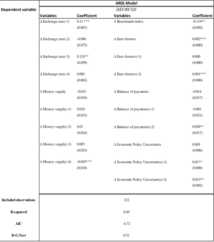
ARDL stands for autoregressive distributed lags, it is a model with adding lags to the dependent together with the independent variables. In this model the fundamental variables were used in addition to number of lags. After 12500 iterations , the lowest AIC, Akaike Information Criteria, was chosen to accept one model ARDL(4,4,0,2,2,2), i.e., four lags of exchange rate (EURUSD), four lags of money supply differentials (M2), no lags of benchmark indexes differentials (IND), two lags of euro futures (Eurofx), two lags of balance of payments differentials (BOP), and two lags of economic policy uncertainty index differentials (EPU).

Table 6.3 shows more significant variables, all variables shows theoretically true

coefficient change affecting dependent variable. For instance, money supply (M2) the first and fourth lag were negatively related with the exchange rate (EURUSD), which is true based on economic theory as shown in Appendix A3. Except for the EPU, it shows an opposite sign, but it showed a granger causality between EPU and BOP. Where granger causality assumes that if BOP was a dependent variable, the EPU granger cause BOP in

1,02 1,04 1,06 1,08 1,1 1,12 1,14 1,16 1,18 1,04 1,06 1,08 1,1 1,12 1,14 1,16 1,18 Actual Forecasted

three lags with a significance level of 0.00, as shown in Table C1 in the Appendix C. In a timeseries, an independent variable granger cause a dependent variable if the lags in the independent variable predicted the future values of the dependent variable (Everitt and Skrondal, 2010). 𝐸𝑈𝑅𝑈𝑆𝐷𝑡 = 𝛽0+ 𝛽1𝐸𝑈𝑅𝑈𝑆𝐷𝑡−1+ 𝛽2𝐸𝑈𝑅𝑈𝑆𝐷𝑡−2 + 𝛽3𝐸𝑈𝑅𝑈𝑆𝐷𝑡−3 + 𝛽3𝐸𝑈𝑅𝑈𝑆𝐷𝑡−4+ 𝛼1𝑀2_𝐷𝐼𝐹𝐹𝑡+ 𝛼2𝑀2_𝐷𝐼𝐹𝐹𝑥𝑡−1+ 𝛼3𝑀2_𝐷𝐼𝐹𝐹𝑡−2+ 𝛼4𝑀2_𝐷𝐼𝐹𝐹𝑡−3+ 𝛼5𝑀2_𝐷𝐼𝐹𝐹𝑡−4 + 𝛼6𝐼𝑁𝐷𝑡+ 𝛼7𝐸𝑈𝑅𝑂𝐹𝑋𝑡+ 𝛼8𝐸𝑈𝑅𝑂𝐹𝑋𝑡−1+ 𝛼9𝐸𝑈𝑅𝑂𝐹𝑋𝑡−2+ 𝛼10𝐵𝑂𝑃_𝐷𝐼𝐹𝐹𝑡+ 𝛼11𝐵𝑂𝑃_𝐷𝐼𝐹𝐹𝑡−1+ 𝛼12𝐵𝑂𝑃_𝐷𝐼𝐹𝐹𝑡−2+ 𝛼13𝐸𝑃𝑈_𝐷𝐼𝐹𝐹𝑡+ 𝛼14𝐸𝑃𝑈_𝐷𝐼𝐹𝐹𝑡−1+ 𝛼₁₅𝐸𝑃𝑈_𝐷𝐼𝐹𝐹_𝑡−2+ ɛ_𝑡 (3)

By adding lags to the dependent and independent variables using the same model of the fundamental model, the model became significant by the fact that the F-Stat prob. Of around 0.000 shows that up to 1% of significance level we may reject the null hypothesis of F-Stat, and conclude that all variables jointly in a model, are significant and do affect the dependent variable.

R-squared has a value of 0.49, the Breusch-Godfrey test (B-G Test) shows an insignificant value of 0.51 where we may not reject the null hypothesis in B-G test which states no autocorrelation hence, we conclude that there is no autocorrelation in our model. For the sample in Table 6.3, ceteris paribus, a one unit increase in the first lag of the exchange rate increase DEURUSD by 0.31 units, a one percent increase relatively in fourth lag of Money supply decrease DEURUSD by 0.045 units, a one percent relatively in the benchmark index decrease DEURUSD by 0.119 units, a one percent increase in the difference between long and short contracts of Euro futures increase DEURUSD 0.001 units, a one unit increase relatively in balance of payments second lag decrease DEURUSD by 0.036 units, a one percent increase relatively in second lag of Economic policy uncertainty increase DEURUSD by 0.013 units. The interpretation was on significant variables of the model.

Table 6.3 Output of ARDL Model

Notes: The Asterisk stands for significance level (*** significant at 0,01 level , ** significant at 0,05 level and * significant at 0,1 level). Negative numbers within brackets in the independent variables’ names are the number of lags. Breusch-Godfrey serial Correlation LM test (B-G Test) result is the prob. of Chi-squared. The letter symbol "∆D" in the beginning of every variable's name stands for the first difference to transform/make the data stationary. All the independent variables above except Exchange Rate lags, are the difference between Euro Area and USA variables and EURO futures are the difference between the long and short contracts. The model’s lags were selected based on the lowest AIC value.

Dependent variable

Variables Coefficient Variables Coefficient

∆Exchange rate(-1) 0.31 *** ∆ Benchmark index -0.119**

(0.067) (0.050)

∆ Exchange rate(-2) -0.096 ∆ Euro futures 0.002***

(0.073) (0.000)

∆ Exchange rate(-3) 0.124** ∆ Euro futures(-1) 0.000

(0.059) (0.000)

∆ Exchange rate(-4) 0.083 ∆ Euro futures(-2) 0.001***

(0.062) (0.000)

∆ Money supply -0.015 ∆ Balance of payments -0.014

(0.019) (0.017)

∆ Money supply(-1) 0.024 ∆ Balance of payments(-1) -0.001

(0.023) (0.021)

∆ Money supply(-2) 0.01 ∆ Balance of payments(-2) 0.036**

(0.024) (0.017)

∆ Money supply(-3) 0.007 ∆ Economic Policy Uncertainty 0.001

(0.023) (0.006)

∆ Money supply(-4) -0.045*** ∆ Economic Policy Uncertainty(-1) 0.01**

(0.018) (0.006)

∆ Economic Policy Uncertainty(-2) 0.013** (0.002) 212 0.49 -4.72 0.51 DEURUSD ARDL Model Included observations R-squared AIC B-G Test

Trying to predict the exchange rate with the variables in Table 5.3, with the ARDL model:

Fig.6.4 First difference of the series Exchange Rate (DEURUSD) and its forecast

In Figure 6.4 the forecasted data was plotted two months forward on the actual exchange rate to visualize the direction accuracy of the forecasted series. It shows that the Forecasted series forecasted the Actual series two months prior the event took place.

6.2 Machine Learning (ML)

Artificial intelligence is the new way of acquiring smart machines to do jobs that would have been conducted otherwise by human intelligence but instead saving us time, resources, increase effectiveness and quality in the data that we retrieve. It is stated in McCrea (2016) that ML is an application of algorithms that learns from experience. The concept is to have computers that do not need to be programmed and basically that learns data from patterns and past events. The data can be in different forms like images, numbers, etc. This method first needs training data that the algorithm learns from after that it finds a pattern in which it proceeds to make predictions according to its learning. This prediction is improved overtime by different techniques, and it learns itself to do so without being programmed. As mention above, one of the best qualities of this model is the absence of human interventions. Once trained, the algorithm can pick up on trends and pattern in the data, process it faster while performing in multi-dimension (Mueller et al

2016). The disadvantage with the model can be that it needs time and resources in order to learn and have accurate result. The data this algorithm needs in order to train is massive

-0,03 -0,02 -0,01 0 0,01 0,02 0,03 0,04 -0,03 -0,02 -0,01 0 0,01 0,02 0,03 0,04 2018M 10 2018M 11 20 18 M 12 2019M 01 2019M 02 2019M 03 2019M 04 2019M 05 2019M 06 2019M 07 2019M 08 2019M 09 2019M 10 2019M 11 2019M 12 2020M 01 2020M 02 2020M 03 2020M 04 2020M 05 2020M 06 2020M 07 Actual Forecasted

and chances are high that the interpretation of the result is sometimes biased or error in general. There are three types of ML:

1. Supervised Machine Learning the machine is given two data. One for training and

the other for testing (Dasgupta & Nath 2016). The algorithms learn the patterns with the result and that is why it takes less time to predict. This machine learning is highly accurate because input and out are given and trained well with the usage of labeled data. This labeled data helps to categorize and analyze data for future accuracy. It is mention in Mueller et al (2016) that the main difference between supervised and unsupervised ML. This learning has two types being regression and classification. In this paper the type of algorithm we will be using is Extreme Gradient Boosting (XGBoost) which is a type of this ML.

2. Unsupervised Machine Learning the data is not labeled nor classified. Unlike

supervised ML, there is only input but not expected output for testing or learning. Ayodele (2010) discusses how the algorithms discover its own result since it does not have any earlier training of the data. There is reward for the right outcome and penalties for the wrong outcomes that helps the machine to discover and learn from itself (Mueller et al 2016).

3. Reinforcement Learning in this type of learning, it is more of algorithm learning

behavior. Since it is behavioral based there is trial and error in which over time it develops prediction (Torrey & Shavlik, 2009).

For this paper, our focus will be on supervised learning as we will be working with ensemble learning which is a type of supervised learning. Ensemble learning is about combining different models that are individually weak to create a model that is strong with accurate predictions by making the prediction less biased and less variance. The main aim of ML algorithms is to get a good prediction which is achieved when the value predicted is equal to the actual value. When we have a difference in those values then that means there is an error in the data. Bias and variance are the two types of error we have in ML. A model with low variance and low bias is needed to be achieved. However, with lower bias we have higher variance and vice versa that is why we have the Bias-variance trade-off.

To understand deeply we will look into bias first. Bias can be defined as the distinction between the standard estimate of our model and the accurate value which we are trying to predict (Neal et al, 2018). High error is expected in the cases where the bias is high caused by the fact that after being trained with certain data, assumptions are made by the model. Those assumptions are not accurate when the testing data are used again. Variance on the contrary is a model considering the variation in the data. It simply means that in this model the data is over analyzing training data that it finds problems with the prediction of the new data. According to Yu (2006) the more input features used with more complexity makes the variance high. But if more training data are used it can be improved. In the case of bias, the features are simplified so by adding more complex features to the model and increasing the output, the bias can be reduced. With optimal complicity, suggested in Jabbar & Khan (2015) we will avoid models that are overfitting (high variance with lower bias) or underfitting (lower variance and higher bias). The concept of variance and bias is important to comprehend because in order to understand the types of ensemble learning the key difference is the amount of bias and variance.

As mentioned in Syarif et al. (2012) ensemble learning is about combining different models to make them strong predictors by making the prediction less biased and less variance. In this paper, we will be aiming at the boosting method as our paper is focused on XGBoost. As discussed by above, boosting method starts with fitted data in linear regression or decision tree. The second tree is built focusing on the area where the previous tree functioned weakly. It is because of this that it learns from its past and transforms weak learners to strong ones. This is the process of boosting where the flaw is corrected from the previous tree. There are two types of boosting method

1) Adaboost or adaptive boosting is the first boosting algorithm. Mayr et al (2014) wrote

that boosting is an area of ensemble learning, so it focuses on the multiple week learners and how it can be combined into one single strong learner. In the case of Adaboost, that deals with classification data, all observations are given equal weight. The base learners are decision trees. It is a type of gradient boosting but more efficient, flexible, and compact which makes it different from traditional boosting systems. The advantage of this boosting method is hyperparameters used help it against data overfitting, stopping additional trees if no improvement in the data is made, being able to start with the model

from where you left off without restarting the process, and the usage of different languages unlike previous boosting methods.

2) XGBoost employs the gradient boosting decision tree algorithm. In support of this

statement, Chen, & Guestrin,(2016) suggested that the best component of XGBoost in machine learning method is the speed. It is a software library supporting many interfaces and characteristics like gradient boosting, stochastic gradient boosting, and regularized gradient boosting. This boost is a decision tree based predicting unstructured data. To understand how the decision tree works we must look deeply on the structure of the algorithm. The decision tree is upside down, with leaves splitting into branches. Those that do not split anymore are the decision leaf. The trees either can be classification trees where the result is short with decision leaf or regression tree which have continuous values like prices. We will be using the XGBoost regressor for our forecasting method. Linear or tree functions are used to adjust individual algorithms with the help of hyperparameters. These hyperparameters can be distinguished into two parameters. Those that set the model characteristics and those that adapt behavior. When tuning the data, we use two tree boasters or linear boasters. What is the difference between these boosters? Well, to put it in a simple way, the first one uses ensemble learning where the later uses a weighted sum of the function. The parameters used in machine learning are the learning rate of the algorithm (eta) is the process of boosting conservative. The eta shrinks the features weight. This shrinkage is after every boosting step. Choosing a lower rate could help us reach the global minimum. Maximum depth of a tree(max_depth) is overfitting and can be prevented by lower value. When this value is high, it could learn the relationship to training data. Usually, small trees are better than big trees with a lot of leaves than it gets complex and the data is overfitted.

Some of XGBoost’s advantages, based on our experience, are:

- Powerful ensemble gradient boosting tree model. - It can train classification and regression models.

Some of XGBoost’s disadvantages, based on our experience, are:

- Needs high computational power to train big models. - Not the best model for time series.

To understand the tree ensemble model, Random forest in our example, look at Figure

6.5. This demonstration is used to simplify the tress work and does not include

mathematical formulas. We can see how more than one tree is used here which yield a better prediction result where a one tree is considered a weak learner (xgboost, n.d.).

Fig.6.5 XGBoost way of using more than a tree for estimation.

Trying to predict the exchange rate using XGBoost model:

(1) 𝐸𝑈𝑅𝑈𝑆𝐷𝑡= 𝛽0 + 𝛽1𝐵𝑂𝑃_𝐷𝐼𝐹𝐹1𝑡 + 𝛽2𝑀2_𝐷𝐼𝐹𝐹2𝑡 + 𝛽3𝐼𝑁𝐷_𝐷𝐼𝐹𝐹3𝑡 + 𝛽4𝐸𝑈𝑅𝐹𝑋4𝑡+ 𝛽4𝐸𝑃𝑈_𝐷𝐼𝐹𝐹5𝑡 + ɛ𝑡 1,08 1,1 1,12 1,14 1,16 1,18 1,2 1,22 1,24 1,26 1,28 1,04 1,06 1,08 1,1 1,12 1,14 1,16 1,18 2018M 10 2018M 11 2018M 12 2019M 01 2019M 02 2019M 03 2019M 04 2019M 05 2019M 06 2019M 07 20 19 M 08 2019M 09 2019M 10 2019M 11 2019M 12 2020M 01 2020M 02 2020M 03 2020M 04 2020M 05 2020M 06 2020M 07 2020M 08 20 20 M 09 Actual Predicted

Fig 6.6 XGBoost - The Actual is the exchange rate through the interval 2018-2020 and the predicted is its prediction.

Equation (1) is reused here which is the fundamental model in Table 6.1, we replicated the same equation but with XGBoost to test if it yields different outcome. We got a different outcome that will be compared in the next part section 6.3.

𝐸𝑈𝑅𝑈𝑆𝐷_𝑡 = 𝛽₀+ 𝛽₁𝐸𝑈𝑅𝑈𝑆𝐷_𝑡−1+ 𝛽₂𝐸𝑈𝑅𝑈𝑆𝐷_𝑡−2 + 𝛽₃𝐸𝑈𝑅𝑈𝑆𝐷_𝑡−3+ 𝛽₃𝐸𝑈𝑅𝑈𝑆𝐷_𝑡−4+ 𝛼₁𝑀2_𝐷𝐼𝐹𝐹_𝑡+ 𝛼₂𝑀2_𝐷𝐼𝐹𝐹𝑥_𝑡−1+ 𝛼₃𝑀2_𝐷𝐼𝐹𝐹_𝑡−2+ 𝛼₄𝑀2_𝐷𝐼𝐹𝐹_𝑡−3+ 𝛼₅𝑀2_𝐷𝐼𝐹𝐹_𝑡−4+ 𝛼₆𝐼𝑁𝐷_𝑡+ 𝛼₇𝐸𝑈𝑅𝑂𝐹𝑋_𝑡+ 𝛼₈𝐸𝑈𝑅𝑂𝐹𝑋_𝑡−1 + 𝛼₉𝐸𝑈𝑅𝑂𝐹𝑋_𝑡−2+ 𝛼₁₀𝐵𝑂𝑃_𝐷𝐼𝐹𝐹_𝑡+

𝛼11𝐵𝑂𝑃_𝐷𝐼𝐹𝐹𝑡−1+ 𝛼12𝐵𝑂𝑃_𝐷𝐼𝐹𝐹𝑡−2+ 𝛼13𝐸𝑃𝑈_𝐷𝐼𝐹𝐹𝑡+ 𝛼14𝐸𝑃𝑈_𝐷𝐼𝐹𝐹𝑡−1+

𝛼₁₅𝐸𝑃𝑈_𝐷𝐼𝐹𝐹_𝑡−2+ ɛ_𝑡 (3)

Fig 6.7 XGBoost - First difference of the series Exchange Rate (DEURUSD) and its forecast

Equation (3) typically follows ARDL model, so it yields the same output. But here XGBoost algorithm adjusted its own parameters based on the Parameters for Tree Booster. The learning rate (eta) was set to 0.05 and nineteen trees with a maximum depth (max_depth) of one. The booster was “gbtree” which is a tree-based model, gradient boosted decision trees.

6.3 Comparison of models

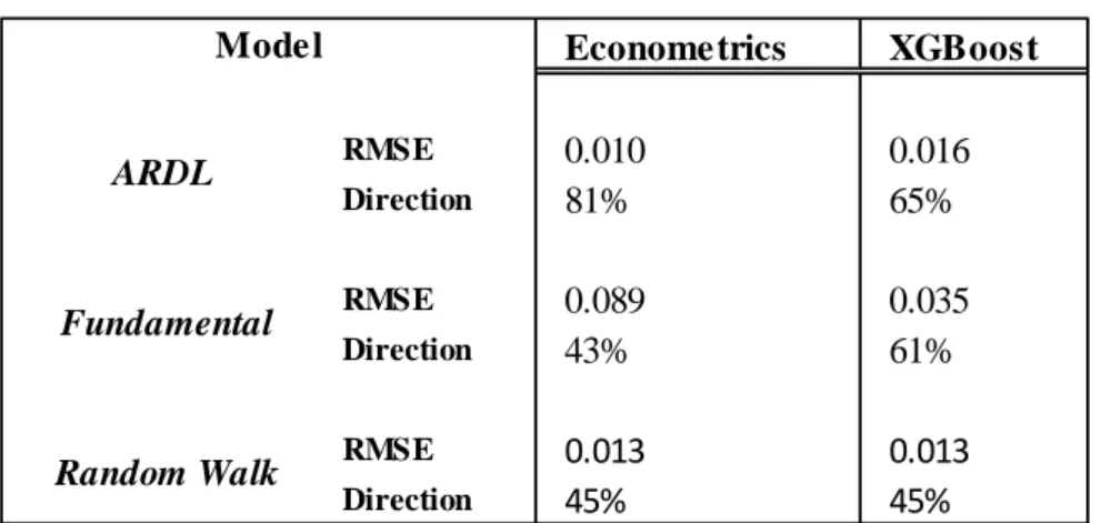
Both measurements of magnitude and direction are shown in Table 6.5. It is obvious that ARDL model based on econometrics have the least RMSE and the highest direction accuracy. -0,02 -0,015 -0,01 -0,005 0 0,005 0,01 0,015 0,02 -0,03 -0,02 -0,01 0 0,01 0,02 0,03 0,04 2018M10 2018M11 2018M12 2019M01 2019M02 2019M03 2019M04 2019M05 2019M06 2019M07 2019M08 2019M09 2019M10 2019M11 2019M12 2020M01 2020M02 2020M03 2020M04 2020M05 2020M06 2020M07 Actual Forecasted

Table 6.4 Measurements of the models

However, ARDL model done in XGBoost did not perform better in forecasting. But in the Fundamental model, XGBoost performed better than Econometrics model in predicting the exchange rate. The random walk model had the worst measures, it is clear by looking at Table 6.4 we can notice that lower RMSE does not yield higher Direction Accuracy, within a model comparison. To test the causation between actual series and forecast, we will use granger causality for both series in comparing ARDL with Random walk. The random walk is transformed to a stationary time series to be able to test it.

Table 6.5 Forecast and Actual Granger Causality in Random Walk model

We can see that the actual series (DEURUSD) is causing the forecast series (D(RW)) with probability of 0.000 where we may reject the null hypothesis in granger causality test which states Actual does not granger cause Forecast. We can conclude that for one period Actual granger cause Forecast.

Table 6.6 Forecast and Actual Granger Causality in ARDL model

Econometrics XGBoost RMSE 0.010 0.016 Direction 81% 65% RMSE 0.089 0.035 Direction 43% 61% RMSE 0.013 0.013 Direction _{45% 45%} Model ARDL Fundamental Random Walk

Null Hypothesis: Prob.

D(RW) does not Granger Cause DEURUSD 0.6935

DEURUSD does not Granger Cause D(RW) 0.0000

Null Hypothesis: Prob.

DEURUSDF does not Granger Cause DEURUSD 0.0196 DEURUSD does not Granger Cause DEURUSDF 0.7804

In Table 6.6 the forecast series is causing the actual with probability of 0.0196 where we may reject the null hypothesis of granger causality test which states forecast (DEURUSDF) does not granger cause actual (DEURUSD). We can conclude that in six periods the Forecast granger caused the Actual.

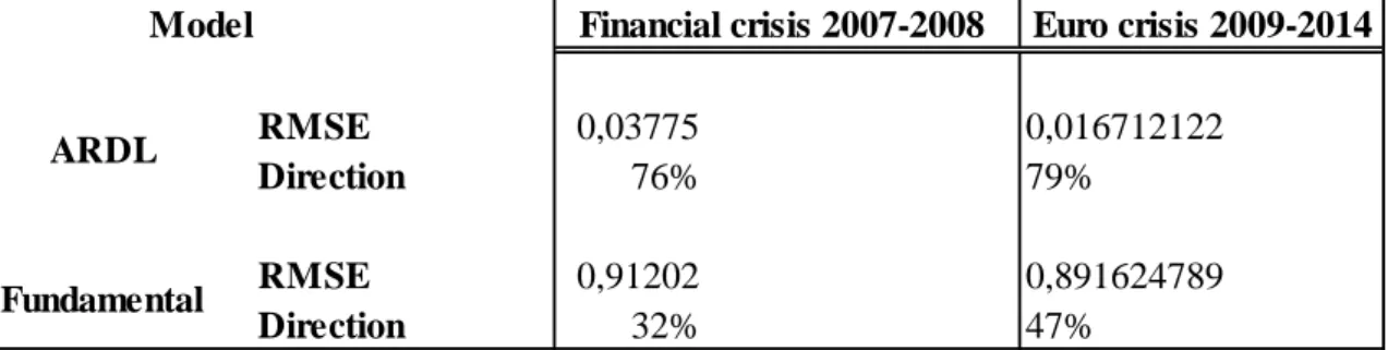
Looking at the previous crisis, we can notice in Figure 6.8 how well the ARDL model performed in predicting the exchange rate (EURUSD). Measurements showed higher than 75% of direction accuracy for ARDL models, Fundamental model is not a good estimator nor forecaster model based on the measurements. We can conclude that lags increased the performance in models, by including previous periods a model will have more weights to consider thus lead to a better estimation and forecasting.

Table 6.7 Measurement of previous crisis prediction

7. Conclusion

Foreign exchange rate impacts world net exports and investments. It is important to know what macroeconomics variables affect the movement of exchange rate in the economies, it is commonly known that macroeconomics uses models to understand the impact of these variables. That is why a good prediction and forecasting is needed. Therefore, we have questioned if a random walk model can be outperformed by other exchange rate models and if it even can forecast. Trying to get a better variables and predictors, a MIDAS model; mixed-data sampling model, could have performed better but the problem is that having higher frequency data like weekly inflation data instead of monthly or monthly GDP data instead of quarterly were not accessible, i.e., such data needs a subscription . So instead of getting high frequency data, we added lags to the model where it included previous periods’ data to the analysis.

Money supply differentials (M2), Balance of payments differentials (BOP), Benchmark indexes differentials (IND), Euro futures long and short contracts differentials (EUROFX), and European policy uncertainty differentials (EPU) are the variables used in our study. Differentials in each variable stands for the difference between Euro Area and the US variables, except for Euro futures the differential stands for the difference between long contracts and short ones. We saw how transforming our data to stationary and adding lags to the variables made it more possible to forecast the target, dependent variable (EURUSD). By eliminating autocorrelation, relationship between error term values disappeared, which showed clearer relation between data thus yielded more accurate results. Euro crisis 2009-2014 RMSE 0,03775 0,016712122 Direction 76% 79% RMSE 0,91202 0,891624789 Direction 32% 47% ARDL Fundamental

Therefore, we tested and compared three models. XGBoost model was not predicting well in comparison to the ARDL model in forecasting. For the Fundamental model, XGBoost performed better after adjustments of the tree booster, it performed better in prediction rather forecasting. These results proved that it could aid in forecasting and predicting the exchange rate that benefit investment funds and federal institutions. Hence, such a success in forecast and prediction in hedge funds and the European financial commission and Federal Trade Commission, eliminates risk and enhances decision making regarding trading and new legislations, respectively.

In future papers we should build recurrent neutral network model (RNN) instead of gradient boosting decision tree like in XGBoost to enhance forecasting performance. We have showed that Random walk model underperformed in forecasting in comparison to other models discussed in this paper based on magnitude and direction measures.

References

Anaraki, N. K. (2007). Meese and Rogoff’s Puzzle revisited. International Review of Business Research Papers, 3(2), 278-304

Ayodele, T. O. (2010). Types of machine learning algorithms. New advances in machine learning, 3, 19-48.

Bash, A. (2016). To hedge or not to hedge foreign exchange exposure: A GCC perspective. International Research Journal of Finance and Economics, 146, 32-42.

Chen, T., He, T., Benesty, M., Khotilovich, V., & Tang, Y. (2015). Xgboost: extreme gradient boosting. R package version 0.4–2, 1-4.

Chen, T., & Guestrin, C. (2016, August). Xgboost: A scalable tree boosting system. In Proceedings of the 22nd acme sigkdd international conference on knowledge discovery and data mining (pp. 785-794).

Cheung, G. W., & Rensvold, R. B. (2002). Evaluating goodness-of-fit indexes for testing measurement invariance. Structural equation modeling, 9(2), 233-255.

Connor, G., & Woo, M. (2004). An introduction to hedge funds.

Commitments of Traders. (n.d.). Retrieved November 13, 2020, from

https://www.cftc.gov/MarketReports/CommitmentsofTraders/index.htm

Cornell, B. (1982). Money supply announcements, interest rates, and foreign exchange.

Journal of International Money and Finance, 1, 201-208

Dasgupta, A., & Nath, A. (2016). Classification of Machine Learning Algorithms. International Journal of Innovative Research in Advanced Engineering (IJIRAE), 3(3), 6-11.

Economic Policy Uncertainty Index. (n.d.). Retrieved November 20, 2020, from https://www.policyuncertainty.com/

Euro Stoxx 50 Historical Rates (STOXX50E). (n.d.). Retrieved October 12, 2020, from https://www.investing.com/indices/eu-stoxx50-historical-data

Evans, M. D., & Lyons, R. K. (2002). Order flow and exchange rate dynamics. Journal

of political economy, 110(1), 170-180.

Everitt, B., & Skrondal, A. (2010). The Cambridge dictionary of statistics, fourth edition. Cambridge University Press.

Frankel, J. A., & Rose, A. K. (1995). Empirical research on nominal exchange rates.

Handbook of international economics, 3, 1689-1729.

Gallo, C. (2014). The Forex market in practice: a computing approach for automated trading strategies. Int. J. Econ. Manag. Sci, 3(169), 1-9.

Ghizoni, S. K. (2013). Creation of the Bretton Woods System. Federal Reserve History. Written as of November, 22.

Gujarati, D. N. (2009). Basic econometrics. Tata McGraw-Hill Education.

HORVATH, Z., & Johnston, R. (2000). AR (1) Time series process. Econometrics 7590

Introduction to Boosted Trees. (n.d.). Retrieved December 27, 2020, from

https://xgboost.readthedocs.io/en/latest/tutorials/model.html

Jabbar, H., & Khan, R. Z. (2015). Methods to avoid over-fitting and under-fitting in supervised machine learning (comparative study). Computer Science, Communication and Instrumentation Devices, 163-172.

Kilian, L., & Taylor, M. P. (2003). Why is it so difficult to beat the random walk forecast of exchange rates?. Journal of International Economics, 60(1), 85-107.

King, M. R., Osler, C. L., & Rime, D. (2011). Foreign exchange market structure, players and evolution.M2 Money Stock. (n.d.). Retrieved October 12, 2020, from

https://fred.stlouisfed.org/series/M2

Laurin, M., & Martynenko, O. (2009). The influence of macroeconomic factors on the probability of default

Makin, A. J. (2002). The balance of payments and the exchange rate.

Mayr, A., Binder, H., Gefeller, O., & Schmid, M. (2014). The evolution of boosting algorithms-from machine learning to statistical modelling. arXiv preprint arXiv:1403.1452.

McCrea, N. (2016). An Introduction to Machine Learning Theory and Its Applications: A Visual Tutorial with Examples

Meese, R. A., & Rogoff, K. (1983). Empirical exchange rate models of the seventies: Do they fit out of sample? Journal of international economics, 14(1-2), 3-24.

Monetary aggregate M2 vis-a-vis euro area non-MFI excl. central gov. reported by MFI & central gov. & post office giro Inst. in the euro area (index). (n.d.). Retrieved October 12, 2020, from

https://sdw.ecb.europa.eu/quickview.do?org.apache.struts.taglib.html.TOKEN=43957c0 4d2325529ad47dc6ade8360cd

Montgomery, D. C., Jennings, C. L., & Kulahci, M. (2015). Introduction to time series analysis and forecasting. John Wiley & Sons.

Moosa, I. A., & Burns, K. (2015). Model Misspecification. In Demystifying the Meese-Rogoff Puzzle (pp. 73-88). Palgrave Pivot, London.

Mueller, J. P., & Massaron, L. (2016). Machine learning for dummies. John Wiley & Sons

Natekin, A., & Knoll, A. (2013). Gradient boosting machines, a tutorial. Frontiers in neurorobotics, 7, 21.

Neal, B., Mittal, S., Baratin, A., Tantia, V., Scicluna, M., Lacoste-Julien, S., & Mitliagkas, I. (2018). A modern take on the bias-variance tradeoff in neural networks. arXiv preprint arXiv:1810.08591.

Refaeilzadeh, P., Tang, L., & Liu, H. (2009). Cross-Validation. Encyclopedia of database systems, 5, 532-538

Roudgar, E. (2012). Forecasting Foreign Exchange Market Trends: Is Technical Analysis Perspective Successful? (Doctoral dissertation, Eastern Mediterranean University (EMU)).

S&P 500 Real Price by Month. (n.d.). Retrieved October 12, 2020, from

https://www.quandl.com/data/MULTPL/SP500_REAL_PRICE_MONTH-S-P-500-Real-Price-by-Month

Stulz, R. M. (1996). Rethinking risk management. Journal of applied corporate finance, 9(3), 8-25.

Syarif, I., Zaluska, E., Prugel-Bennett, A., & Wills, G. (2012, July). Application of bagging, boosting and stacking to intrusion detection. In International Workshop on Machine Learning and Data Mining in Pattern Recognition (pp. 593-602). Springer, Berlin, Heidelberg.

Taylor, M. P., & Peel, D. A. (2000). Nonlinear adjustment, long-run equilibrium and exchange rate fundamentals. Journal of international Money and Finance, 19(1), 33-53.

Torrey, L., & Shavlik, J. (2010). Transfer learning. In Handbook of research on machine learning applications and trends: algorithms, methods, and techniques (pp. 242-264). IGI global

Truman, E. M. (2017). The End of the Bretton Woods International Monetary System. Peterson Institute for International Economics Working Paper, (17-11).

Uriel, E. (2013). Introduction to Econometrics. Electronic textbook. Version, 9, 2013

U.S. / Euro Foreign Exchange Rate. (2020, August 02). Retrieved August 15, 2020, from https://fred.stlouisfed.org/series/EXUSEU

Yu, L., Lai, K. K., Wang, S., & Huang, W. (2006, May). A bias-variance-complexity trade-off framework for complex system modeling. In International Conference on

Appendix

A.

Fig. A1 EURUSD (Black) EUROFX, the Euro futures based in Chicago Mercantile (Gray). EUROFX has a positive relation with EURUSD.

Fig. A2 EURUSD (Black) DIFF, balance of payments difference (Euro Area - USA) (Gray). BOP-DIFF has a negative relation with EURUSD.

Fig. A3 EURUSD (Black) IND-DIFF, benchmark index difference (STOXX 50 - S&P 500) , (Gray). The index has a negative relation with EURUSD.

Fig. A4 EURUSD (Black) M2-DIFF, money supply difference between Euro area and USA, (Gray). We can notice that money supply has a negative relationship with EURUSD.

Fig. A5 EURUSD (Black) EPU, Economic Policy Uncertainty (Gray). EPU has a negative relation with EURUSD

B.

Multicollinearity (Variance Inflation Factors) of ARDL model.

Variable VIF ∆Exchange rate(-1) 1.747935 ∆ Exchange rate(-2) 1.981737 ∆ Exchange rate(-3) 1.428089 ∆ Exchange rate(-4) 1.308743 ∆ Money supply 1.169522 ∆ Money supply(-1) 1.181912 ∆ Money supply(-2) 1.282097 ∆ Money supply(-3) 1.221235 ∆ Money supply(-4) 1.225670 ∆ Benchmark index 1.106837 ∆ Euro futures 1.234216 ∆ Euro futures(-1) 1.738439 ∆ Euro futures(-2) 1.710484 ∆ Balance of payments 1.223000 ∆ Balance of payments(-1) 1.289089 ∆ Balance of payments(-2) 1.140892

∆ Economic Policy Uncertainty 1.217001

∆ Economic Policy Uncertainty(-1) 1.340201

C.

Table C1 Granger Causality (3 lags included)

Table C2 Fundamental Model correlation matrix

Table C3 ARDL Model correlation matrix

Null Hypothesis: Prob.

BOP_DIFF does not Granger Cause EPU_DIFF 0.739 EPU_DIFF does not Granger Cause BOP_DIFF 0.015

DEURUSD M2_DIFF IND_DIFF DEURFX BOP_DIFF EPU_DIFF

DEURUSD 1 M2_DIFF -0,09 1 IND_DIFF -0,11 -0,05 1 DEURFX 0,51 0,00 0,10 1 BOP_DIFF 0,01 0,07 -0,05 0,03 1 EPU_DIFF 0,00 0,08 -0,12 -0,05 -0,09 1

DEURUSD DEURUSD(-2) DEURUSD(-3) DEURUSD(-4) M2_DIFF M2_DIFF(-1) M2_DIFF(-2) M2_DIFF(-3) M2_DIFF(-4) IND_DIFF DEURFX DEURFX(-1) DEURFX(-2) BOP_DIFF BOP_DIFF(-1) BOP_DIFF(-2) EPU_DIFF EPU_DIFF(-1) EPU_DIFF(-2)

DEURUSD 1 DEURUSD(-2) 0,011 1 DEURUSD(-3) 0,016 0,298 1 DEURUSD(-4) 0,062 0,017 0,303 1 M2_DIFF -0,088 -0,124 -0,055 -0,065 1 M2_DIFF(-1) -0,027 -0,052 -0,122 -0,051 0,186 1 M2_DIFF(-2) 0,155 -0,088 -0,046 -0,117 0,142 0,188 1 M2_DIFF(-3) 0,063 -0,028 -0,085 -0,042 0,113 0,142 0,189 1 M2_DIFF(-4) -0,033 0,144 -0,038 -0,092 0,143 0,106 0,134 0,183 1 IND_DIFF -0,111 -0,052 0,003 -0,027 -0,048 0,021 -0,013 0,013 -0,032 1 DEURFX 0,513 -0,264 -0,160 0,005 0,002 0,045 0,236 0,038 0,066 0,099 1 DEURFX(-1) 0,169 -0,075 -0,265 -0,159 -0,050 -0,001 0,044 0,235 0,037 -0,063 0,068 1 DEURFX(-2) 0,161 0,509 -0,077 -0,266 -0,041 -0,052 -0,003 0,042 0,237 -0,041 -0,059 0,068 1 BOP_DIFF 0,007 -0,011 0,138 0,110 0,065 0,039 -0,098 0,021 0,085 -0,047 0,033 -0,037 -0,108 1 BOP_DIFF(-1) -0,015 0,028 -0,012 0,148 -0,143 0,057 0,041 -0,105 0,011 0,061 0,001 0,027 -0,042 -0,237 1 BOP_DIFF(-2) 0,118 0,000 0,028 -0,012 0,045 -0,142 0,057 0,042 -0,104 -0,005 -0,001 0,002 0,028 -0,040 -0,237 1 EPU_DIFF 0,000 -0,026 0,039 -0,004 0,077 -0,080 0,030 0,038 -0,088 -0,111 -0,044 -0,026 -0,025 -0,092 -0,084 0,062 1 EPU_DIFF(-1) 0,037 0,084 -0,018 0,041 -0,085 0,085 -0,076 0,035 0,033 0,051 -0,034 -0,041 -0,026 0,115 -0,076 -0,086 -0,315 1 EPU_DIFF(-2) 0,050 0,001 0,087 -0,012 -0,061 -0,088 0,088 -0,077 0,027 -0,010 -0,029 -0,037 -0,045 0,064 0,105 -0,074 -0,026 -0,306 1

Table C4 Descriptive statistics

EURUSD BOP_DIFF M2_DIFF IND_DIFF EUROFX EPU_DIFF

Mean 1,215 0,010 0,002 -0,005 5,933 -0,016 Median 1,227 0,011 0,003 -0,004 11,180 -0,010 Maximum 1,576 0,454 0,354 0,078 48,575 0,675 Minimum 0,853 -0,314 -0,388 -0,121 -52,220 -1,244 Std. Dev. 0,161 0,085 0,085 0,026 24,660 0,268 Skewness -0,303 0,210 0,145 -0,575 -0,543 -0,527 Kurtosis 2,746 6,519 6,245 5,347 2,313 4,423 Jarque-Bera 4,301 125,063 105,695 68,002 16,443 31,210 Probability 0,116 0,000 0,000 0,000 0,000 0,000 Sum 290,384 2,476 0,417 -1,135 1418,060 -3,788 Observations 239 239 239 239 239 239