Estimating the economic lifetime of roads
using road replacement data
Mattias Haraldsson
a,∗, Lina Jonsson
b aVTI - Swedish National Road and Transport Research Institute, Box 55685, SE-102 15 Stockholm, Sweden
b
VTI - Swedish National Road and Transport Research Institute, Box 55685, SE-102 15 Stockholm, Sweden
Abstract
This paper analyses the economic lifetime of roads in Sweden using a data over kilometres of new roads together with a “centrality” index constructed from popu-lation statistics. The repopu-lation between economic lifetime and centrality is performed by poisson regression. It is shown that roads in more central parts of the country and in parts more affected by population changes (increase) generally have shorter economic lifetimes. The analysis shows economic lifetimes of Swedish roads to be between 25 and 111 years, with the majority of the economic lifetimes in the upper part of this range (above 70 years).
Key words: Economic lifetime, road, cost benefit analysis
Sammanfattning
I denna rapport analyseras den ekonomiska livsl¨angden f¨or svenska v¨agar. Den ekonomiska livsl¨angden definieras som den period under vilken ett v¨agobjekt har en viss funktion vilket i sin tur beror p˚a dess roll i
v¨agtransportsystemet, samt vilken standard den har. F¨or¨andringar av detta inneb¨ar att den ekonomiska livsl¨angden bryts. Det datamaterial som
∗ Corresponding author. Tel.: +46 (0)8 555770 24.
Email addresses: mattias.haraldsson@vti.se(Mattias Haraldsson),
anv¨ands visar hur mycket ny europa- och riksv¨ag som byggs ˚arligen i V¨agverkets olika driftomr˚aden. Med “ny” avses s˚adant som V¨agverket betraktar som nybyggnad i sin bokf¨oring. Uppgifterna om nybyggnad j¨amf¨ors med m¨angden befintlig europa- och riksv¨ag. Observationerna ¨ar h¨amtade fr˚an driftomr˚aden i samtliga V¨agverksregioner f¨orutom Stockholm. Relationen mellan ny och befintlig v¨ag ger under vissa antaganden en uppfattning om ekonomisk livsl¨angd, vilket utnyttjas i rapporten. Under f¨oruts¨attning att en ny eller ombyggd v¨ag inneb¨ar att funktionen hos en gammal v¨ag ¨andras ger antalet kilometer ny v¨ag en uppskattning av antalet kilometer v¨ag med avslutad ekonomisk livsl¨angd. Analysen utg˚ar fr˚an hypotesen att den ekonomiska livsl¨angden p˚averkas av v¨agens n¨arhet till omr˚aden med stor folkm¨angd eller till omr˚aden d¨ar folkm¨angden f¨or¨andras snabbt. I dessa fall kommer behoven av olika v¨agar att ¨andras relativt snabbt, vilket kan g¨ora de ekonomiska livsl¨angderna kortare. I rapporten ber¨aknas ett index som f¨or varje driftomr˚ade visar hur centralt omr˚adet ¨ar. Centraliteten i ett visst driftomr˚ade beror p˚a befolkning i alla driftomr˚aden viktat med avst˚and. Centralitetsm˚attet ber¨aknas f¨or flera ˚ar vilket g¨or att f¨or¨andringen ¨over tiden kan ber¨aknas. Det visar sig att centralitet och
centralitetsf¨or¨andring ¨ar n¨ara korrelerade. Centralitets¨okningen ¨ar snabbast i omr˚aden som redan ¨ar centrala, vilket ¨ar en indikation p˚a demografisk
koncentration. Centralitet och centralitetsf¨or¨andring anv¨ands i tv˚a separata regressionsmodeller till att f¨orklara skillnader i ekonomisk livsl¨angd.
Eftersom m˚atten ¨ar n¨ara korrelarade ger de ocks˚a likande resultat. Hypotesen att den ekonomiska livsl¨angden p˚averkas av centralitet eller f¨or¨andring av centralitet bekr¨aftas. Den ekonomiska livsl¨angden ¨ar kortare i omr˚aden med h¨og centralitet eller snabb centralitetstillv¨axt.
Den skattade modellen ger ekonomiska livsl¨angder p˚a mellan 25 och 111 ˚ar. Majoriteten av v¨agarna har livsl¨angder i den ¨ovre delen av detta intervall. Ur praktisk synvinkel inneb¨ar detta att kalkylperioden i cost benefit
analyser, som brukar best¨ammas utifr˚an uppskattningar av den ekonomiska livsl¨angden, med vissa undantag b¨or vara t¨amligen l˚ang. Den generellt rekommenderade kalkylperioden i V¨agverkets riktlinjer ¨ar idag 60 ˚ar. Den analys som presenteras h¨ar motiverar ingen s¨ankning av detta v¨arde. En differentiering av kalkylperioderna p˚averkar kalkylresultaten lite i omr˚aden med l˚ag centralitet. En ¨okning fr˚an det generella v¨ardet 60 ˚ar betyder p.g.a. diskontering troligtvis lite f¨or kalkylresultatet. Eventuella restv¨ardesber¨akningar blir d¨armed mindre betydelsefulla. F¨or objekt i omr˚aden med h¨og centralitet eller snabb centralitetsh¨ojning ¨ar d¨aremot kostnader och nyttor bortom den f¨orsta ekonomiska livsl¨angden viktiga. V˚ar rekommendantion ¨ar att kalkylperioden d¨ar s¨atts till tv˚a ekonomiska
livsl¨angder och att en ny trafikprognos g¨ors f¨or den andra halvan av kalkylperioden (den andra ekonomiska livsl¨angden).
Acknowledgements
This paper is a result of a data collection process in which several persons at Swedish Road Administration were involved. The authors would like to thank Anneli Persson and Martin Risberg (Sk˚ane), Hakan Jansson (M¨alardalen), Jan-˚Ake Karehed (Syd¨ost), Rolf Olsson (V¨ast), Peter Jakobsson (Mitt) and Leena Bj¨ornstr¨om (Norr).
1 Introduction
The economic lifetime of a road (or any other real capital object) is the period during which it maintains its function. That is, the road does not have to be worn out in a technical sense to have reached the end of its
economic lifetime1
. Further use of the road is possible, but it will then have another function. In many cases however, the new road will be built on the same place as the old one, probably using the old construction as a part of the new.
To be able to observe when the function of a road has changed it is of course very important to have a clear understanding of the concept function. Our definition of a specific function includes both a description of a) the role of the road in the transport system, e.g. being the main road connection between points A and B, and b) a description of its standard (width, safety etc.). Changes in a) are induced by substitution of another object, probably a completely new road, for the present one. The present road might still be used but it will have another role. Changes in b) mean that a present road is modified in a way that changes its standard profoundly, e.g. widening it and adding another lane. That a change in a) means an economic lifetime has ended is probably uncontroversial. What standard changes (b) should be enough for the economic lifetime to be considered ended might be open to discussion. The empirical analysis below uses objects considered as
construction in the Swedish Road Administrations accounting system. A theoretical possibility is that new roads in a more genuine sense are built, i.e constructed to enable trips between points that have not been connected by road before. But this is probably rare. With few exceptions it is possible to travel by road between any two places. Hence, for our analysis, we assume that whenever we can observe a new road we know that the economic
lifetime of an old road has come to its end.
Why then does an economic lifetime end, that is how can a change in
1
The technical lifetime is the time during which a specific object, that is a piece of hardware/road can be used before it is worn out. An object has one technical lifetime during which it can have one or several functions.
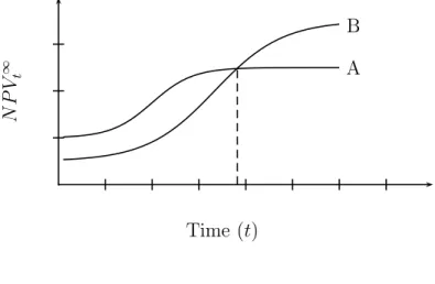
function be explained? Consider the cost benefit analysis of a case where a road is being planned. Two alternatives with the same role but different standards are available. Alternative A is a road which fulfils capacity, safety and other needs at a quite low cost. Alternative B is a road with a higher standard, but, given its higher investment cost, its net present value is lower compared to A. As a consequence, A is built. As time passes by conditions change. The population might rise, with increasing transports as a
consequence. Moreover valuations of safety, comfort and environmental assets might also change. The situation is illustrated in figure 2. To begin with (t = 0) we have alternatives A and B, and A has the higher net present value (NPV). Road A is then built but we recompute the NPV for A and B continuously into the future. The rapid rise in NPV for A (for t > 0) reflects the fact that the investment cost is sunk. After some time (probably quite long), conditions change in a way that NP VB is higher than NP VA and the
economic lifetime of A is finished.
The change in NP V , and finally the ending of an economic lifetime, is explained above by changing circumstances. We can thus expect economic lifetimes to be shorter in areas where conditions change rapidly and where this development is hard to predict. One hypothesis is that population
Fig. 1. The development of NPV and the determination of the economic lifetime
Time (t) N P V ∞ t B A
factors affect the economic lifetime. In areas with a large population or a rapidly changing (growing) population, economic lifetimes are supposedly shorter. The purpose of this paper is to scrutinize this hypothesis empirically. This hypothesis corresponds to the methods used in practice. In an official guide to cost benefit analysis the Swedish Road Administration assumes that 40 years is a reasonable assessment of the economic lifetime of roads close to urban areas, unless the population increase is predicted to be very low in which case 60 years is recommended. (SRA, 2006) We collect data on the economic lifetime, relate this to measures derived from
population variables and get a relation that shows an economic lifetime with a potential geographic variation.
Besides the the potential geographic variation, it is reasonable to believe that roads of different type have different economic life lengths even if
located in the same area. However, this aspect of economic lifetime variation is not analysed in this report.
Earlier research on the economic lifetime of roads is scarce. Grudemo (1996) made an analysis based on a study of all roads constructed in the Swedish regions J¨amtland and Halland after 1945. The two regions are selected to represent the north and south of Sweden respectively. A difference between these two regions is that J¨amtland is less densely populated than Halland. He found that several roads have had an economic lifetime shorter than 40 years in Halland as compared to none in J¨amtland, a finding in line with the hypothesis explored in this paper. He also studied major roads (E4 and E6 through ¨Osterg¨otland and Halland and roads passing by or through the cities Link¨oping, G¨avle, V¨anersborg and Trollh¨attan.
The analysis in this paper shows that roads in more central parts of the country, or in parts more affected by population changes generally have shorter economic lifetimes. The estimated models predict economic lifetimes
of between 25 and 111 years for Swedish roads, with the majority of the predicted values in the upper part of this range (above 70 years).
The rest of this section is devoted to a discussion about how to use knowledge about economic lifetimes. The following two sections contain descriptions of the method and data used in this paper. Thereafter we present the methodology and use this in the analysis. The paper closes with a discussion of the results.
1.1 The relevance of economic lifetime estimates
How should knowledge about economic lifetimes be used? Does the potential variation in economic lifetimes imply that the appraisal period of cost
benefit analysis should vary? If the future was known, i.e. no uncertainty about the stream of costs and benefits existed, the technical lifetimes, i.e. the period during which the object can be used at all, would be the natural appraisal period. No matter if the function of the road changed and several economic lifetimes were contained in the technical lifetime. Since all future costs and benefits were known, it would be natural to include them in the cost benefit analysis.
But the future, with few exceptions, is uncertain. It is thus not clear if and how the infrastructure will be used during its entire technical lifetime. Various changes might alter the original function of the object to something unknown, with uncertain costs and benefits. An appraisal period shorter than the technical lifetime is often used to handle this uncertainty. Bickel (2006) states that “due to uncertainty about traffic, impacts on the environment, safety issues etc., the evaluation period is often shorter than the (technical) lifetime of the infrastructure”. In an analysis situation one has to decide the point in time beyond which the costs and benefits of an
object become so uncertain that they should be left outside the analysis or be approximated by a lump residual value.2
The determination of this point is often based on arguments concerning the economic lifetime. This point determines the appraisal/evaluation period. It varies between 20 years and infinity in Europe (Odgaard et al., 2005). The Swedish Road Administration recommends 40-60 years. (SRA, 2006). After the end of the first economic lifetime, a residual value can be used. Apparently, inclusion of a correctly estimated residual value is more important if the appraisal period is short. When using a long appraisal period the residual value belongs to the far and heavily discounted future. Thus, using differentiated (sometimes short) appraisal periods (set equal to the economic lifetime) requires more focus on residual values.
2 Method
A definition of an economic lifetime based on cost-benefit analyses is given above. By this definition the economic lifetimes ends when it is economically feasible to build another road or make changes in the present one. In reality though, the function might change before or after the economical optimal point, since decision making is often influenced by other arguments as well. The following empirical analysis is made without any attention to the reasons for the change in function. When a change in function is observed, the economic lifetime is over as far as the analysis in this paper is concerned. At least two ways to obtain an empirical measure of the economic lifetime exist. The most obvious is of course to follow roads over time and observe how long they keep their original function. Such data, however, are rarely compiled. To get the information one turns to archives and old documents.
2
Lacking better alternatives, the residual value is often approximated by a share of the original investment cost (see e.g. SVV, 2006; Bickel, 2006; ASEK, 2008).
This was the method used by Grudemo (1996) and is henceforth referred to as “the duration method”. Although one learns a lot about about the reasons for an ended economic lifetime, and gets a very precise economic lifetime of the specific road, this method has the obvious drawback of being very time consuming. As a consequence the number of observations becomes limited, which in turn makes generalization difficult. Also, with few observations it is impossible to assess the uncertainty in the estimates of the economic
lifetimes. We use a more aggregate approach, where we analyse a panel data covering all of Sweden. Comparing the number of kilometers of new roads in regions with the length of the existing network, we get a notion about the speed with which roads are replaced. This is called “the frequency method”. It might seem odd to talk about frequency when analysing a distance
variable (km). But consider the road network as a set of one kilometre sections. Ask then how many of these sections ended their lifetimes during a year. The answer to this question is clearly a frequency, a number of road sections. We can relate this measure to the kilometres of existing road and get a replacement rate which can be transformed into an estimate of the economic lifetime.
2.1 A simple simulation
We now illustrate the duration and frequency methods using a simulated data set. We simulate 15000 units of road. If each unit represents one kilometre, the total length of the simulated data is approximately equal to the “national” and “european” part of the Swedish national road network. Each unit has an independent economic lifetime T drawn from an
exponential distribution with E[T ] = 50. Each road section is renewed 20 times. What we get is 15000 series with time points where the economic lifetimes come to an end. The simulated data is complete (15000
observations) until the first section finishes its 20:th economic lifetime. The repeated economic lifetimes of 10 road units are illustrated in figure 2.1. The vertical bars mark points in time where economic lifetimes are ended.
Fig. 2. Repeated economic lifetimes for a set of roads
0 100 200 300 400 500 600 700 800 || | | 36 || |6 14 39| | | | | 14 | | | | | | | | | | 2 5 2 | | | | | | | | | | | | || | | | |21 54| | | | | | | || | | | || | | | | | | | | | | | | | | || | ||| | | | | | | | | | | | | | | | | | | | | | | | | | | | | || | || | || Time (t) R oa d s
Now, let us look at the duration and frequency methods to estimate the economic lifetime using this data. In both cases we look at a subset (sample) of all simulated roads. Using the duration method we measure the (last) economic lifetime of each road and compute an average over all roads in the sample. Changing to the frequency method we count the number of lifetimes (in the sample) that end over some limited period, compute the replacement rate and then invert to get the economic lifetime.
A rough estimate of the average economic lifetime can be achieved just by counting the ended economic lifetimes (the bars) within the shaded area in figure 2.1 which is 17. Since there are 10 roads and the sample period is 100 years, this means that 1.7 percent (17/10 ∗ 100 = 0.017) of the roads are renewed every year. This in turn implies an average economic lifetime of 59
years (1/0.017 ≈ 59), which is not very far from the true 50 years given the small size of the sample.
Using a larger sample we get better estimates. The results are shown in table 1. First we estimate the economic lifetimes using the duration method, i.e., we follow a limited number (100 and 1000) of roads over time, observe their economic lifetimes and compute a mean which is our estimate.
Standard errors are given by repetition of this procedure 1000 times. To assess the frequency method we count the numbers of roads that are
replaced during a limited period (10 and 30 years) and compare them to the number of roads in the sample (and the length of the period). The result is the share of replaced roads. The inverse of this share is used as a economic lifetime estimate and its standard error is, as before, estimated by repetition of the procedure. As can be seen from the table it is probably a better strategy (the standard error is smaller) to see how large a share of the complete road network is replaced during a ten year period than to follow 100 roads during their entire economic lifetimes.
Table 1
Estimates from simulated data
Duration approach Frequency approach
Last economic lifetime All roads
nr obs 100 roads 1000 roads 10 years 30 years
ˆ
T 50.21 50.08 49.70 50.12
Std error 5.15 1.62 3.45 3.09
2.2 Measuring the number of ended lifetimes - a proxy
We have shown above that the frequency with which roads in the network end their economic lifetimes can be used to estimate the length of these lifetimes. But how do we measure this frequency? In the following empirical analysis we assume that the observed number of kilometres of new roads is a
just proxy for the kilometres of roads with ended economic lifetimes. Although we are interested in the end of an economic lifetime, we use data that describes the construction of new roads. Given our assumption that these replace old roads, the construction of a new road is the same as the end of the economic lifetime of the old one. The question then is whether the length of the old road can be measured by the length of the new. If “new” means improved in some sense, i.e. the old road’s function is transformed by increased width etc., this is certainly true. Besides, the length of the road network is constant in this case.
What if the new road has a different position than the old one? Then, measuring the length of the old road by the length of the new one is an approximation, and as such subject to error. We cannot assess the size of this error, but might justify the approximation by the fact that the straight line distance between A and B is constant. Thus the difference in length is probably not very large and hopefully zero on average.
3 Data
3.1 New roads
The information concerning new roads originates from the regional offices of the Swedish Road Administration (SRA). Each regional office except the region of Stockholm (6 in total) reported all the objects in their area in a period ranging from at most 1990 to 2007 that can be considered as road construction according to the definitions used in SRA:s accounting system.3
Their reports include the total length of each road construction object and
3
PT 31 contains new construction of freeways, multi-lane roads, broad two-lane roads, normal two-lane roads, narrow roads and environmentally, traffic safety pri-oritized roads or streets and public transport routes. Thomas (2004) Roads for pedestrians and bicyclists were excluded.
descriptions of its nature and location. The different regional offices have reported construction for different years, from 9 years of reported
construction to at most 18 years. Each of the road construction objects has been assigned to a maintenance delivery unit (MDU). A MDU is the smallest geographical area that the Road Administration reports statistics for. In total the Swedish road network consists of 131 MDU:s; we have gathered information about road construction from 124. Information concerning the length of the existing road network in every MDU is also taken from the Swedish Road Administration. The existing road network consists of
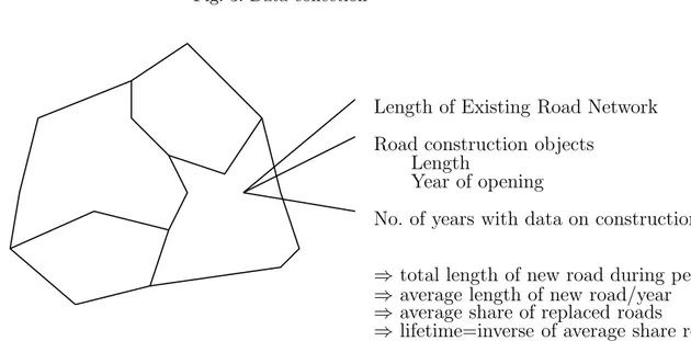
national and ”European” roads, regional roads and local roads. The lifetime estimates are based on the share of national and ”European” roads that are replaced each year within each MDU. Figure 3 illustrates the data collection.
Compared to earlier studies our data is more extensive, covering almost all of Sweden (except Stockholm) A drawback of the data is the rather hight level of aggregation . MDU:s are quite large areas within which the economic life length can be expected to vary considerably.
Fig. 3. Data collection
Length of Existing Road Network Road construction objects
Length
Year of opening
No. of years with data on construction ⇒ total length of new road during period ⇒ average length of new road/year ⇒ average share of replaced roads
⇒ lifetime=inverse of average share replaced The construction of a new road is a quite rare occurrence and looking at a
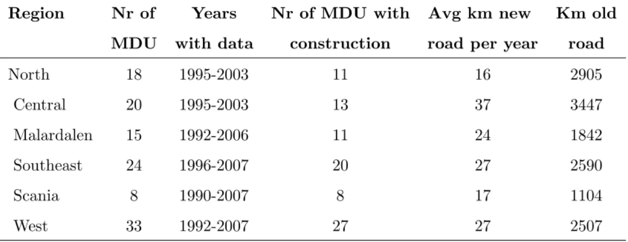
single year only a small minority of the MDU:s experienced any construction and thereby substitution of the road network. For some of the MDU:s there was no road construction at all during the period that our study covers. Table 2 summarizes the available data on road construction divided by region. A comparison between the second and fourth columns shows that in many MDU:s no new roads were built during the observation period.
3.2 Explanatory variables-Centrality
Statistics Sweden provides information about the population of all Swedish built-up areas (t¨atort) with more than 200 inhabitants for the years 1990, 1995, 2000 and 2005. For 2005 the population in these areas sums up to 7.6 million people and thereby represents the majority of the Swedish
population4
. The population is aggregated to the same geographical areas as the lifetime data (MDU). The built-up area population of a MDU is denoted pi. There are N built-up areas. In space these units are represented by a
point (x,y) which enables computation of the distance di,j between each pair
of MDU:s5
. Using a simple gravitation measure (see for instance Hagget (1983)) summed over all relations, a centrality index for each MDU is
4
The total population was 9.2 million people in November 2007
5
di,j is set to one where i = j.
Table 2
Descriptive Statistics
Region Nr of Years Nr of MDU with Avg km new Km old
MDU with data construction road per year road
North 18 1995-2003 11 16 2905 Central 20 1995-2003 13 37 3447 Malardalen 15 1992-2006 11 24 1842 Southeast 24 1996-2007 20 27 2590 Scania 8 1990-2007 8 17 1104 West 33 1992-2007 27 27 2507
computed as: ci = N X j=1 pipj d2 i,j (1)
This measure is computed for 1990, 1995, 2000 and 2005 and we use an average over all these years in the analysis. It is also possible to see how the centrality in different MDU:s has changed between 1990 and 2005. Centrality and change in centrality are closely correlated with a positive sign. The centrality thus increases most in places where centrality is high. Thus we have a trend where the centrality differences are getting larger.
4 Econometric method
We will estimate a function that describes the relation between the number of kilometer new roads (interpreted as ended economic lifetimes of old roads, see above) and centrality/change in centrality. Since our dependent variable is a count in the form of meters of new road, we utilize poisson regression for the estimation. The poisson regression is estimated by the maximum
likelihood method departing from the probability density function:
P (y) = e
−µ
µy
y! (2)
where y is kilometers of new road. In essence, with poisson regression the mean parameter, µ, is made a function of explanatory variables, in this case centrality (change), c. We also control for differences in road network size and the number of observed years. The expected number of meters of new road, y, in a network of specific length, d, over a specific number of years, t, is:
E[y|d, t, c] = µ = exp(α + ln(d) + ln(t) + βc) = dtexp(α + βc) (3)
Network length and the number of years are exposure/offset variables. The poisson distribution has the quite restrictive property that its expected value equals the variance. If this is not a reasonable assumption for the data, poisson regression still results in consistent parameter estimates. The correct covariance matrix is then achieved with robust estimation (Cameron and Triveldi, 1998).
The rate by which the road network is renewed can be interpreted in terms of economic lifetime. To enable this, we exploit the relation between the rate of the count data process and the waiting time in a lifetime model. This relation is exact for poisson/exponential distributions but also holds asymptotically for all other related count data/lifetime
distributions. (Lancaster, 1990) The estimated economic lifetime of a road is the inverse of its estimated rate of new road investments6
: \ E[T |c] = 1 \ E[y|c] = 1 b µ = 1 exp(α +b β)b = exp(−α −b b βc) (4) 5 Analysis
This section takes a closer look at the relationship between the number of new roads and centrality (change) and derive lifetime-centrality (change) relations.
6
The confidence interval can be computed using the delta method (see for instance Greene, 1997)
5.1 Calculated lifetimes and centrality
The share of roads (replacement rate) that is being replaced within each MDU each year is computed as the ratio between the kilometers of new road and the length of the existing network. Then “raw” lifetimes are computed as the inverse of this replacement rate, which works well except in cases where no roads have been replaced at all. No lifetime estimate can be
calculated if the area has seen no road construction. The replacement rate is then zero and the implied economic lifetime infinite. To avoid this, the lifetime estimates are based on the average annual length of new opened roads. Local office reports cover varying numbers of years, which means that the average annual length of new roads is calculated based on different years for each region. The calculated lifetime for each MDU ranges from less than 15 years to more than 10 000 years. In some of the MDU:s no construction has occurred during our investigated period and therefore no lifetime can be calculated.
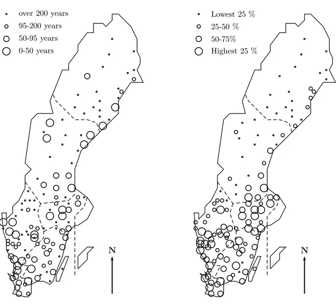
Figure 5.1 shows two maps over lifetimes and centrality. The lifetime map shows MDU:s grouped according to their calculated lifetimes and the MDU:s without any road replacement have been put into the group with the longest lifetimes. The centrality map shows the MDU:s divided into four groups, this time based on their average centrality over the years 1990 to 2005.
Comparing the maps of calculated lifetimes and centrality shows some concordance where the MDU:s with the highest centrality often have the shortest lifetimes and vice versa.
Another way of visualizing how the distribution of calculated lifetimes varies between MDU:s with different centrality is by histograms shown in figure 5.
Fig. 4. Economic lifetimes and centrality N over 200 years 95-200 years 50-95 years 0-50 years Economic lifetimes N Lowest 25 % 25-50 % 50-75% Highest 25 % Centrality (average 1990-2005)
Instead of using the calculated lifetimes directly, an ordinal lifetime variable is created where the group with the longest lifetimes includes observations for which no lifetimes have been calculated because of a lack of construction in that area during the investigated period. The grouping overlaps the previous grouping used in the maps in figure 5.1 with the only difference that the groups with the longest and shortest lifetimes have been divided into two groups. The reason for using lifetime grouping, instead of the lifetimes directly, is to include the observations for the MDU:s without
construction as well. The centrality variable has also been grouped into six groups based on the percentile ranking. The histogram clearly shows that the areas with low centrality have a greater share of MDU:s with very long lifetimes compared to the high centrality groups. Figure 5 thereby supports the hypothesis that lifetimes vary between areas with different centrality.
5.2 Estimating lifetimes
This section uses a more formal method to explore the relation between economic lifetime and centrality (change). We have estimated two different Poisson regression models, one where centrality (average over 1990, 1995, 2000 and 2005) is used as a regressor and one where the change in centrality between 1990 and 2005 is used. The rate of road investments, which can be predicted from the poisson model, is then inverted. The transformed model shows the relation between economic lifetime and centrality (change). Both models produce similar results, which is expected given the close
correlation between centrality and centrality change. It is difficult to give the coefficients of these quite constructed variables a precise and quantitative
0 .2 .4 .6 .8 0 .2 .4 .6 .8 0
0−30 years 30−50 years 50−95 years 95−200 years 200−540 years over 540 år
7 0
0−30 years 30−50 years 50−95 years 95−200 years 200−540 years over 540 år
7 0
0−30 years 30−50 years 50−95 years 95−200 years 200−540 years over 540 år
7
very low centrality low centrality medium low centrality
medium high centrality high centrality very high centrality
Calculated Lifetime Calculated Lifetime Calculated Lifetime
Calculated Lifetime Calculated Lifetime Calculated Lifetime
Density
Calculated Lifetime
Graphs by centrality group
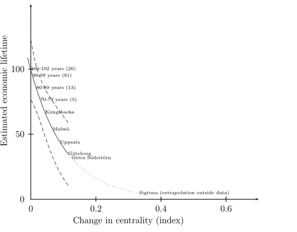
interpretation. But the results show (table 3) that centrality or centrality change has a significantly negative influence on economic lifetimes which are high where centrality (change) is low and vice versa. The estimated economic lifetimes are shown in figures 6 and 7. The solid lines show estimations over the range supported in the data. Dotted lines indicate extrapolation outside the range of our data. The estimated lifetimes are quite unevenly distributed over the range 35-102 years (centrality change model) and 25-111 years (average centrality model). The majority of the MDU:s have their lifetimes in the upper ends of these ranges. A few, which are all located close to large cities, have economic lifetimes below 60 years (both models).
Compared to the “raw” lifetimes computed directly from the observed share of renewals, the fitted models do not produce the highest values. Although present in the data, these values are not influential enough to affect the estimated models very much.
Table 3
Economic lifetime models (transformed poisson regression)
Variable Centrality change Average centrality
β/t β/t Centrality -9.141 change (-2.67) Average -3.070 centrality (-2.99) Constant 4.603 4.705 (38.83) (36.86) N 120 120 6 Discussion
This analysis contributes one step towards knowledge about the economic lifetimes of roads and their geographical variation. We depart from a
Fig. 6. Estimated (by change in centrality) economic lifetimes with 95 percent confi-dence bands. Dotted line indicates extrapolation outside range of data. The number of MDU:s with economic lifetimes in different ranges is shown within parentheses.
0 0.2 0.4 0.6 0 50 100 100-102 years (26) 90-99 years (81) 80-89 years (13) 70-79 years (5) Kungsbacka Malm¨o Uppsala G¨oteborg ¨
Ostra S¨odert¨orn
Sigtuna (extrapolation outside data)
Change in centrality (index)
E st im at ed ec on om ic li fe ti m e
hypothesis saying that the economic lifetime is affected by population factors. The economic lifetime of a road at a specific point is affected by population not only at that point but in surrounding areas as well. Using a simple gravity formula we have constructed a centrality measure to
summarize these factors. We estimate a model that explores the relation between economic lifetime and the centrality measure as well as a model where the change in centrality is the explanatory variable. The models show that the economic lifetime of a road is affected by centrality (change); the higher the centrality (change), the shorter the economic lifetime. The estimated lifetimes for different Swedish regions are quite unevenly
distributed over the range 35-102 years (centrality change model) and 25-111 years (average centrality model). The majority of the MDU:s have their lifetimes in the upper ends of these ranges. A few MDU:s, which are all
Fig. 7. Estimated (by centrality) economic lifetimes with 95 percent confidence bands. Dotted line indicates extrapolation outside range of data. The number of MDU:s with economic lifetimes in different ranges is shown within parentheses.
0 0.25 0.50 0.75 1.00 1.25 0 50 100 ¨ OrebroHelsingborg V¨aster˚as Malm¨o Uppsala ¨
Ostra S¨odert¨orn
G¨oteborg
Sigtuna (extrapolation outside data) 100-111 years (83)
90-99 years (11) 80-89 years (9)
70-79 years (9)
Average centrality (index)
E st im at ed ec on om ic li fe ti m e
located close to large cities, have economic lifetimes below 60 years (both models).
What do our findings imply for practical cost benefit analysis? Given the praxis to set the appraisal period equal to one economic lifetime, a pretty long appraisal period would be the general recommendation for Sweden. The economic lifetime model show that most roads can be expected to maintain their original function for quite long time and the appraisal period should be quite long accordingly. Today, 60 years is recommended in official road CBA guidelines, and our analysis does not support a reduction of that value. The long economic lifetimes mean that the future use of the roads are pretty straightforward to predict and also that the residual values are not very
important. They will be heavily discounted, so the crude methods for residual value approximation is not a big problem.
More care is necessary in high centrality areas where the short economic lifetimes of roads imply that conditions are fast changing and that the point in time when the function of a road changes is not far away. A
recommendation is to use an appraisal period with twice the length of the economic lifetime in areas with high centrality (change)7
and do separate prognoses for these two economic lifetimes. Because of the rapidly changing conditions in these areas it is risky to rely on simple prediction models (e.g. to assume traffic to increase by a certain percentage per year) for longer periods, which is otherwise common. In high centrality areas we would recommend that a more thorough analysis of traffic demand etc. is done not only for a year in the beginning of the planning period but for one or more future years as well.
References
ASEK: 2008, ‘ASEK 4’. Technical report, Arbetsgruppen f¨or Samh¨allsekonomiska Kalkylv¨arden. In Swedish, Draft.
Bickel, P.: 2006, ‘Proposal for Harmonised Guidelines’. Deliverable 5, HEATCO.
Cameron, A. C. and P. K. Triveldi: 1998, Regression analysis of count data, Econometric society monographs. Cambridge university press.
Greene, W. H.: 1997, Econometric Analysis. Prentice Hall, 3:rd edition. Grudemo, S.: 1996, ‘V¨agars ekonomiska livsl¨angd’. Notat 13:1, VTI. In
Swedish.
Hagget, P.: 1983, Geography A Modern Synthesis. Harper Collins.
7
Lancaster, T.: 1990, The econometric analysis of transition data, No. 17 in Econometric society monographs. Cambridge University Press.
Odgaard, T., C. Kelly, and J. Laird: 2005, ‘Current practice in project appraisal in Europe’. Deliverable 1, HEATCO.
SRA: 2006, ‘V¨agverkets samh¨allsekonomiska kalkylv¨arden’. Publ 127, V¨agverket. In Swedish.
SVV: 2006, ‘Konsekvensanalyser- veiledning’. H˚andbok 140, Statens vegvesen. In Norwegian.
Thomas, F.: 2004, ‘Swedish Road account - M¨alardalen 1998-2002’. Report 500A, VTI.