Statistical Learning and
Analysis on
Homology-Based Features
JENS AGERBERG
KTH ROYAL INSTITUTE OF TECHNOLOGY SCHOOL OF ENGINEERING SCIENCES
on Homology-Based Features
JENS AGERBERG
Degree Projects in Mathematical Statistics (30 ECTS credits) Master's Programme in Applied and Computational Mathematics KTH Royal Institute of Technology year 2020
Supervisor at RISE SICS: Ather Gattami
Supervisors at KTH: Martina Scolamiero, Wojciech Chachólski Examiner at KTH: Martina Scolamiero
TRITA-SCI-GRU 2020:056 MAT-E 2020:019
Royal Institute of Technology
School of Engineering Sciences
KTH SCI
SE-100 44 Stockholm, Sweden URL: www.kth.se/sci
Stable rank has recently been proposed as an invariant to encode the result of persistent homology, a method used in topological data analysis. In this thesis we develop methods for statistical analysis as well as machine learning methods based on stable rank. As stable rank may be viewed as a mapping to a Hilbert space, a kernel can be constructed from the inner product in this space. First, we investigate this kernel in the context of kernel learning methods such as support-vector machines. Next, using the theory of kernel embedding of probability distributions, we give a statistical treatment of the kernel by showing some of its properties and develop a two-sample hypothesis test based on the kernel. As an alternative approach, a mapping toRdwith
learnable parameters can be conceived, serving as an input layer to a neural network. The developed methods are first evaluated on synthetic data. Then the two-sample hypothesis test is applied on the OASIS open access brain imaging dataset. Finally a graph classification task is performed on a dataset collected from Reddit.
med homologibaserad data
Sammanfattning
Stable rank har föreslagits som en sammanfattning på datanivå av resultatet av persistent homology, en metod inom topologisk dataanalys. I detta examensarbete
utvecklar vi metoder inom statistisk analys och maskininlärning baserade på stable rank. Eftersom stable rank kan ses som en avbildning i ett Hilbertrum kan en kärna konstrueras från inre produkten i detta rum. Först undersöker vi denna kärnas egenskaper när den används inom ramen för maskininlärningsmetoder som stödvektormaskin (SVM). Därefter, med grund i teorin för inbäddning av sannolikhetsfördelningar i reproducing kernel Hilbertrum, undersöker vi hur kärnan kan användas för att utveckla ett test för statistisk hypotesprövning. Slutligen, som ett alternativ till metoder baserade på kärnor, utvecklas en avbildning i Rd med
optimerbara parametrar, som kan användas som ett ingångslager i ett neuralt nätverk. Metoderna utvärderas först på syntetisk data. Vidare utförs ett statistiskt test på OASIS, ett öppet dataset inom neuroradiologi. Slutligen utvärderas metoderna på klassificering av grafer, baserat på ett dataset insamlat från Reddit.
I would like to thank Martina Scolamiero and Wojciech Chachólski at KTH for introducing me to the field of topological data analysis and being so generous with their time, support and engagement in this work.
I would also like to thank Ather Gattami at RISE for valuable feedback and guidance throughout the thesis.
1 Introduction
1
1.1 Background . . . 1
1.2 Objective . . . 2
1.3 Organization . . . 3
2 Background and related work
4
2.1 Persistent homology . . . 42.1.1 Point clouds and distance spaces . . . 4
2.1.2 Simplicial complexes . . . 5
2.1.3 Homology on simplicial complexes . . . 6
2.1.4 Vietoris-Rips . . . 7
2.1.5 Parametrized simplicial complexes and tameness . . . 8
2.1.6 Bar decomposition . . . 9
2.1.7 Pseudometrics on persistence diagrams . . . 11
2.2 Stable rank . . . 11
2.2.1 Contours . . . 11
2.2.2 Pseudometrics on tame parametrized vector spaces . . . 12
2.2.3 Stable rank . . . 13
2.2.4 Ample stable rank . . . 14
2.3 Statistical approaches for persistent homology . . . 15
2.3.1 Introduction . . . 15
2.3.2 Overview of approaches . . . 16
2.4 Hilbert spaces, RKHS and kernels . . . 17
2.4.1 Real Hilbert spaces . . . 17
2.4.2 Kernels . . . 18
2.5 Kernel embedding of probability distributions . . . 19
2.5.1 Maximum Mean Discrepancy . . . 19
2.5.2 MMD and RKHS . . . 19
2.5.3 Universality . . . 20
2.6 Empirical estimates and hypothesis test . . . 21
2.6.1 Empirical estimates . . . 21
2.6.2 Two-sample hypothesis test . . . 22
2.6.3 Distribution of test statistic . . . 22
2.7 Scale-space kernel. . . 23
2.8 Machine learning . . . 24
2.8.1 Kernel methods . . . 24
2.8.2 Artificial neural networks . . . 24
2.8.3 Sets as inputs to neural networks . . . 25
2.9 Persistent homology and machine learning . . . 26
2.9.1 Introduction . . . 26
2.9.2 Overview of approaches . . . 27
2.9.3 Learnable parameters . . . 29
2.9.4 Stability . . . 30
3 Kernel-based learning and statistical analysis
31
3.1 Introduction . . . 313.2 Restrictions on parametrized vector spaces . . . 32
3.3 Interpretation of the restrictions . . . 32
3.4 Constructing the kernels. . . 33
3.5 Stability of the kernels . . . 34
3.5.1 First kernel . . . 34
3.5.2 Second kernel . . . 35
3.5.3 Comment on the stability of kernels . . . 35
3.6 Kernel methods for machine learning . . . 36
3.7 Computing the kernel . . . 37
3.8 RKHS and probability embedding . . . 37
3.9 Universality . . . 38
3.10 Compactness . . . 39
4 Neural network input layer
44
4.1 Introduction . . . 44
4.2 Parametrized families of contours . . . 45
4.3 Stable rank for parametrized families . . . 45
4.4 Towards neural network input layers . . . 46
4.5 Discretizing the y-axis . . . 47
4.6 Properties of the discretization . . . 48
4.7 Constructing neural network architectures . . . 50
4.8 Implementation . . . 51
5 Experiments
53
5.1 Kernel-based statistical test . . . 535.1.1 Geometric shapes . . . 53
5.1.2 OASIS dataset . . . 56
5.2 Machine learning . . . 61
5.2.1 Point processes . . . 61
5.2.2 Graph classification . . . 65
6 Conclusion and future work
71
Introduction
1.1 Background
Topological data analysis (TDA) constitutes a novel framework for data analysis, mathematically well-founded and with roots in algebraic topology. Through the method of persistent homology, TDA proposes to analyze datasets, often high-dimensional and unstructured, but where each observation is a space that encodes some notion of distance. An example of such space is a point cloud, which is produced for instance by 3D scanners. Persistent homology represents such spaces through a combinatorial object, a parametrized simplicial complex, from which topological features can be computed at various spatial resolutions. Such topological summaries, which can be seen as the output of persistent homology, are robust to perturbations in the input data and their efficient computation has been made possible by readily available tools. In recent applications, and in such varied fields as bioinformatics [36] and finance [22], it has been shown to encode valuable information, often orthogonal to that derived from non-topological methods.
To take the data analysis further, one would like to introduce a statistical framework, for instance to be able to consider probability distributions over topological summaries and infer their properties based on samples. Alternatively, the discriminative information contained in the topological summaries makes them interesting in the context of machine learning, for instance to serve as input in supervised learning problems. The space of topological summaries – called persistence diagrams – while endowed with a metric, suffers from computational challenges and lacks the structure
of a Euclidean or more generally Hilbert space often desired for the development of machine learning methods. For these reasons, much of the recent efforts to develop statistical methods for topological summaries have been devoted to crafting mappings from the space of persistence diagrams to spaces where statistical concepts are well-founded. Such mappings need to be stable, i.e. robust to perturbations in the input, computationally efficient and retain the discriminative information of the summaries.
Instead of considering mappings from the space of persistence diagrams, Chachólski and Riihimäki [11] propose to work in the space of parametrized vector spaces, obtained during the computation of persistent homology. This space can be endowed with various metrics and possesses a discrete invariant, called rank. The authors propose a hierarchical stabilization of the rank leading to a new invariant, stable
rank, with a richer geometry. By construction, the stable rank encodes the metric,
chosen to compare parametrized vector spaces. Except for a proof of concept supplied in [11], stable rank has yet to be adapted to a statistical framework or be used for machine learning problems. The approach is however believed to present advantages. Indeed, instead of a complete representation of persistence, as in the case of persistence diagrams, stable rank allows to choose a suitable metric to highlight properties of a particular dataset and problem at hand. For instance for a classification problem, a metric that discriminates well between classes could be chosen. As stable rank constitutes a mapping into Lp spaces, many statistical methods can be
envisioned.
1.2 Objective
Our objective in this thesis is to develop methods in statistical analysis and learning for persistent homology, based on stable rank. More specifically:
1. We first construct kernels based on stable rank: as stable rank may be viewed as a mapping to a Hilbert space, a kernel can be constructed from the inner product in this space. Such a kernel can be used in the context of kernel learning methods such as support-vector machines (SVM).
2. Such kernels can also be used for statistical analysis, motivated by the theory of kernel embedding of probability distributions. We will show how this embedding
justifies the construction of hypothesis tests based on the kernel, which can be used to determine if two samples of outputs of persistent homology can be said to originate from the same probability distribution.
3. Finally, as an alternative to kernel approaches, we conceive a mapping with learnable parameters to Rd, serving as an input layer to a neural network.
Optimizing the parameters of such mapping can be seen as a way to find an optimal metric for a problem at hand, within the framework of stable rank.
1.3 Organization
In chapter2the relevant background and related work is presented. In chapter3the kernels based on stable rank are described, and their use in the context of machine learning methods and kernel-based statistical methods is motivated. In chapter4the input layer to a neural network, derived from stable rank, is described. Chapter 5
contains the experiments. First, the statistical tests are performed on synthetic data and on the OASIS open access brain imaging dataset. Second, the machine learning methods are evaluated on synthetic data and on a graph classification task based on a dataset collected from Reddit. Finally chapter6summarizes the thesis and discusses future directions.
Background and related work
2.1 Persistent homology
2.1.1 Point clouds and distance spaces
The most fundamental way of encoding spatial information is via distances. A distance on a set X is by definition a function d: X × X → R such that it is non-negative d(x, y)≥ 0, symmetric d(x, y) = d(y, x) and reflexive d(x, x) = 0 for all x and y in X. If in addition triangle inequality holds, i.e. d(x, y) + d(y, z) ≥ d(x, z), for all x, y, z in X, then such a distance d is called a metric. For example the function that assigns to two elements x and y in Rn the number!(x
1− y1)2+· · · + (xn− yn)2 is the well-known
Euclidean metric. This is only one of many possible distances onRn.
A point cloud is by definition a finite subset of Rn with the distance given by the
restriction of a chosen distance on Rn. More generally, distance spaces can encode
a notion of distance (or similarity) between a finite set of points, e.g. in a pairwise distance matrix.
Such structures are often outcomes of experiments and measurements done during experiments. They are the main class of objects that topological data analysis aims at understanding through the method of the persistent homology. In this thesis the main running theme is to study statistical behaviour of homology-based invariants extracted from distance spaces.
Although distances are convenient in encoding outcomes of experiments, they are not convenient in extracting homology of the representing spatial information. For that
purpose simplicial complexes will be used. Moreover, some data, such as graphs or polygon meshes, can be directly modeled as simplicial complexes, as is demonstrated in some of the experiments in chapter5.
2.1.2 Simplicial complexes
A collection K of finite and non-empty subsets of X is called a simplicial complex (on X) if:
• {x} belongs to K for any x in X.
• if σ belongs to K, then so does any non empty subset of σ.
An element σ = {x0, . . . , xn} in a simplicial complex K is called a simplex of dimension
n.
The subset of K consisting of simplices of dimension n is denoted by Kn. Elements of
K0are referred to as vertices and elements of K1as edges.
For example the collection ∆[X], of all finite subsets of X, is a simplicial complex. Let K be a simplicial complex on X and L be a simplicial complex on Y . Then a function f : K → L is called a map of simplicial complexes if for every σ in K there is a function f0: X → Y such that f(σ) = {f0(x) s.t. x in σ} belongs to L.
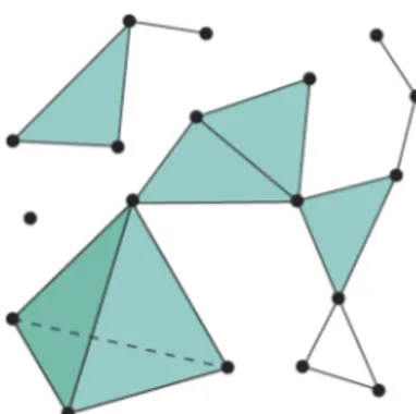
Simplicial complexes are combinatorial objects which encode spatial information in a way which is convenient for extracting homology. An example simplicial complex is shown in Figure2.1.1.
2.1.3 Homology on simplicial complexes
Our first step in defining homology is to move from simplicial complexes to vector spaces. In this thesis we are going to consider only homology with coefficients in the field F2 of two elements. Let K be a simplicial complex and n a natural number. We define F2Knto be the F2-vector space with Knas its base. Explicitly:
F2Kn=⊕σ∈KnF2. (2.1)
Our next step is to define, for n > 0, a linear function on bases elements:
∂n: F2Kn→ F2Kn−1
∂n(σ) :=
"
τ⊂σ,τ∈Kn−1
τ. (2.2)
In addition, set ∂0 to be the zero function ∂0 = 0 : F2K0 → 0. The composition
∂n◦ ∂n+1is the zero function for all natural numbers n. This implies that Im(∂n+1) ⊂
Ker(∂n). Elements in Ker(∂n) are called cycles and elements in Im(∂n+1) are called
boundaries.
We can thus define the following quotient vector space, which is called the n-th homology of K:
Hn(K) := Ker(∂n)/Im(∂n+1). (2.3)
Homology measures how many cycles which are not also boundaries there are. The dimension of Hn(K), dim(Ker(∂n))− dim(Im(∂n+1)), called the n-th Betti number, is
of particular importance as it can be interpreted as capturing the number of topological features of the simplicial complex, e.g. number of connected components for H0(K),
number of holes for H1(K) and similarly for n > 1.
linear function fn: F2Kn → F2Lnon bases elements as follows: fn(σ) := ⎧ ⎪ ⎨ ⎪ ⎩ f (σ) if f(σ) is a simplex of dimension n,
0 if f(σ) is a simplex of dimension strictly smaller than n. The sequence consisting of the linear functions fn: F2Kn → F2Ln indexed by the
natural numbers makes the following diagram commutative for every positive n:
F2Kn+1 F2Kn
F2Ln+1 F2Ln ∂n+1
fn+1 fn
∂n+1
Hence fnmaps boundaries and cycles of K into respectively boundaries and cycles of
L, and thus induces a linear map on the homology. We denote this linear function as:
Hnf : HnK → HnL.
The assignment f (→ Hnf satisfies the following properties: it preserves the identity
Hn(id) = id and it commutes with compositions Hn(f ◦ g) = (Hnf ) ◦ (Hng) for
any composable maps f and g of simplicial complexes. This means that homology is a functor transforming simplicial complexes and their maps into vector spaces with linear functions as morphisms.
2.1.4 Vietoris-Rips
We have so far discussed homology of simplicial complexes. While this can be interesting in its own right, the goal as introduced in2.1.1is often to study homology (and further homology-based invariants and its statistical properties) of distance spaces. In doing so we need a translation step that transforms distance information into a simplicial complex. In this thesis we focus on Vietoris-Rips construction for this purpose.
Let d be a distance on a finite set X. Choose a non-negative real number t in [0, ∞). Then the collection:
V Rt(X, d) :={σ ⊂ X s.t. σ is finite and d(x, y) ≤ t for all x, y ∈ σ} (2.4)
is a simplicial complex called the Vietoris-Rips complex of the distance d at time t. In words, all subsets of X where all elements are at distance at most t of each other will form simplices. Note that if s < t, then there is an inclusion VRs(X, d) ⊂ VRt(X, d)
which is a map of simplicial complexes. Note further that since X is finite, there is t such that VRt(X, d) = ∆[X]. Vietoris-Rips at time t is illustrated in Figure2.1.2.
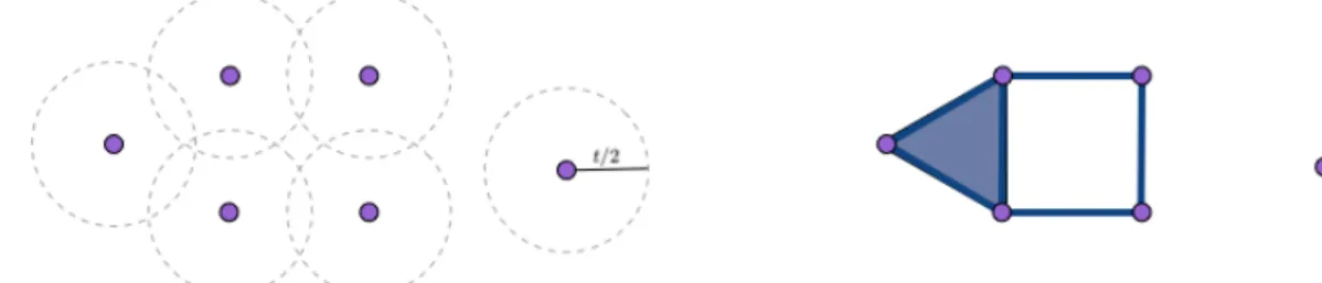
Figure 2.1.2: Left: six purple points together with balls of radius t
2allowing to judge the
distance between the points. Right: the Vietoris-Rips complex at time t. The points form simplices of dimension 0, the blue lines correspond to simplices of dimension 1 and the filled triangle corresponds to a simplex of dimension 2.
2.1.5 Parametrized simplicial complexes and tameness
Let d be a distance on a set X. The family of maps between Vietoris-Rips complexes of a given distance {VRs(X, d) ⊂ VRt(X, d)}s<t∈[0,∞) is an example of a [0,
parametrized simplicial complex, which we denote simply by VR(X, d). A [0, ∞)-parametrized simplicial complex K is by definition a functor indexed by the poset category [0, ∞), of non negative real numbers, with values in the category of simplicial complexes. Explicitly, a [0, ∞)-parametrized simplicial complex is a sequence of simplicial complexes {Ks}s∈[0,∞), indexed by [0, ∞), together with a sequence of maps
{Ks<t: Ks → Kt}s<t∈[0,∞), indexed by s < t in [0, ∞), such that Ks<tKr<s = Kr<t, for
every r < s < t in [0, ∞).
By taking homologies we can transform a [0, ∞)-parametrized simplicial complex into a [0, ∞)-parametrized vector space V . Explicitly a parametrized vector space is a collection of vector spaces {Vs}s∈[0,∞) together with maps between vector spaces
{Vs<t : Vs → Vt}s<t∈[0,∞)for s < t in [0, ∞) such that Vs<tVr<s = Vr<t, for every r < s < t
If X is a finite set, then this parametrized vector space satisfies additional tameness conditions:
1. Vsis finite-dimensional for any scale s in [0, ∞).
2. There is a finite sequence 0 < t0 < ... < tkof elements in [0, ∞) such that for s ≤ t
in [0, ∞), a transition map Vs≤t may fail to be an isomorphism only if s < ti ≤ t
for some i. Such a sequence t0, ..., tkis called a discretizing sequence of size k + 1.
Note that a sequence t0, ..., tk discretizes a tame parametrized vector space V , if and
only if the restrictions of V to the subposets [0, t0), …, [tk−1, tk), [tk,∞) are isomorphic
to the constant functors.
We denote the set of tame parametrized vector spaces as Tame([0, ∞), Vect).
Proposition 1. Let V be a tame parametrized vector space. Then there is a unique
minimal (with respect to the size) discretizing sequence for V .
Proof. We can assume that the parametrized vector space V is not constant, otherwise
t = {∅} is a discretizing sequence of size zero and therefore the unique minimal discretizing sequence for V . The set X of all sequences discretizing V is not empty and its elements have size at least one, since V is tame and non-constant. Let τ = {τi}ki=0
be an element in X of minimal size, i.e. |τ| ≤ |x|, ∀x ∈ X. By minimality of τ and the fact that it is a discretizing sequence, for each τi ∈ τ there exists (ai, bi) ∈ [τi−1, τi+1)
such that Vai<bi is not an isomorphism and ai < τi < bi. It follows that Vs<t is also not an isomorphism for ai ≤ s < τi < t≤ bi.
We will prove that τ ⊂ x, ∀x ∈ X. Thus this discretizing sequence can be characterized as τ = 'x∈Xx and is therefore unique. Suppose there exists τ′ such that τ is not a subset of τ′. In particular there exists τ
i ∈ τ such that τi ̸= τ ′ j for all τ ′ j ∈ τ ′. Define ϵ = minj|τi − τ ′
j|. Then for a = max{ai, τi− 2ϵ} and b = min{bi, τi+ 2ϵ}, we have that
Va<b is not an isomorphism although there is no τj′ in the interval [a, b), contradicting
the hypothesis that τ′ is a discretizing sequence for V .
2.1.6 Bar decomposition
Our goal is now to move towards a representation of the n-th persistent homology useful for data analysis. We start by defining the parametrized vector space K(s, e):
K(s, e)a := ⎧ ⎪ ⎨ ⎪ ⎩ K if s ≤ a < e, 0 otherwise, K(s, e)a≤b := ⎧ ⎪ ⎨ ⎪ ⎩ id if dim(K(s, e)a) = dim(K(s, e)b) = 1, 0 otherwise. (2.5)
These are indecomposable tame parametrized vector spaces and hence constitute the simplest possible objects of this class. One of the fundamental theorems in Persistent homology [55] shows that any V ∈ Tame([0, ∞), Vect) is isomorphic to a direct sum
(n
i=1K(si, ei). Such collections of bars are called barcodes and can be represented as
multisets of elements in the upper half-plane, that is a collection of points {(si, ei) s.t.
(si, ei)∈ R2, ei > si}ni=1for some n where all elements (si, ei) need not be unique. Such
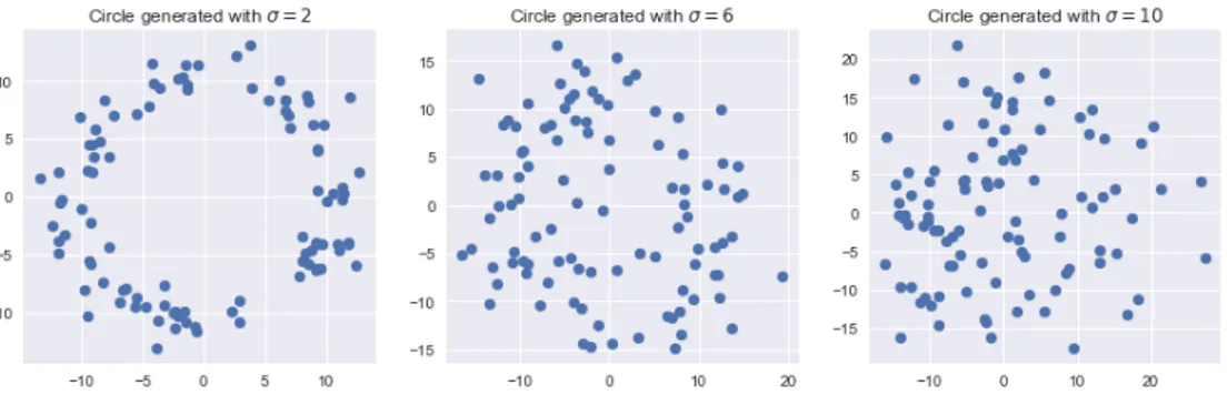
multisets constitute a form of topological summary called persistence diagrams and denoted by D. From a persistence diagram plotted in the plane, one can read off when (in the sense of the filtration scale, e.g. t for Vietoris-Rips above) ”topological features” appeared (si) and how long they persisted (i.e. ei−siif ei <∞, if ei =∞ the topological
feature persists forever and is called essential), as well as how many such features there were (the multiplicity of (si, ei)). An example of a persistence diagram, generated from
Vietoris-Rips filtration of a point cloud representing a noisy circle, is shown in Figure
2.1.3.
Figure 2.1.3: Left: a point cloud representing a noisy circle. Middle: the persistence diagram for the H1 homology resulting from the Vietoris-Rips filtration of the point
cloud. Right: stable rank with standard contour for H1 homology resulting from the
2.1.7 Pseudometrics on persistence diagrams
We call D the set of extended persistence diagrams, that is composed of elements d∪∆ where d ∈ D and ∆ = {(x, y) ∈ R2 s.t. x = y} where each point in ∆ has infinite
multiplicity.
D can be endowed with the Wasserstein metric defined as:
Wp(d1, d2) := (inf γ " x∈d1 ||x − γ(x)||p∞) 1 p. (2.6)
Where d1, d2 ∈ D and γ is the set of all bijections from d1 to d2. Different p
correspond to different metrics, for p = ∞ it is called the bottleneck metric. The addition of the diagonal can be motivated by observing that points of the diagonal have zero persistence, thus one can say that the information contained in the persistence diagrams is not altered, while such addition makes it possible to define the metric in terms of bijections betweeen sets as those sets now have the same cardinality.
2.2 Stable rank
2.2.1 Contours
A wide class of metrics can also be defined directly on Tame([0, ∞), Vect). We start by defining contours of distance type (for other types of contours see [11]) and will then explain how such contours lead to pseudometrics on Tame([0, ∞), Vect).
We let f : [0, ∞) → [0, ∞) be a Lebesgue measurable function with strictly positive values, called a density. We further let Cf(a, ϵ) be the function Cf : [0,∞] × [0, ∞) →
[0,∞] defined by the following integral equation if a < ∞:
ϵ =
) Cf(a,ϵ)
a
f (x)dx (2.7)
and by Cf(∞, ϵ) := ∞. Then Cf is called a contour (of distance type) and has the
following properties for all a and b in [0, ∞] and ϵ and τ in [0, ∞): 1. If a ≤ b and ϵ ≤ τ, then Cf(a, ϵ)≤ Cf(b, τ ),
3. Cf(Cf(a, τ ), ϵ) = Cf(a, τ + ϵ),
4. Cf(−, ϵ) : [0, ∞] → [0, ∞] is a monomorphism for every ϵ in [0, ∞),
5. Cf(a,−) : [0, ∞) → [0, ∞] is a monomorphism whose image is [a, ∞) for every a
in [0, ∞).
The contour defined by the density f(x) = 1 is called the standard contour. We note that the equation above reduces to ϵ = *Cf(a,ϵ)
a 1dx = Cf(a, ϵ) − a and thus
Cf(a, ϵ) = a + ϵ.
2.2.2 Pseudometrics on tame parametrized vector spaces
For a contour Cf, a pseudometric can now be defined for V, W ∈ Tame([0, ∞), Vect),
and ϵ ∈ [0, ∞) in the following way:
1. A map h : V → W is called an ϵ-equivalence with respect to Cfif for any a ∈ [0, ∞)
s.t. Cf(a, ϵ) < ∞, there is a linear function Wa → VCf(a,ϵ) making the following diagram commutative: Va VCf(a,ϵ) Wa WCf(a,ϵ) Va≤Cf (a,ϵ) ha hCf (a,ϵ) Wa≤Cf (a,ϵ)
2. V and W are called ϵ-equivalent with respect to Cf if there is a X ∈
Tame([0, ∞), Vect) and maps g : V → X ← W : h s.t. g is an ϵ1-equivalence,
h is an ϵ2-equivalence and ϵ1 + ϵ2 ≤ ϵ.
3. Let S := {ϵ ∈ [0, ∞) s.t. V, W ϵ-equivalent }. Then we define the distance:
dCf(V, W ) := ⎧ ⎪ ⎨ ⎪ ⎩ ∞ if S = ∅, inf(S) if S ̸= ∅. (2.8)
2.2.3 Stable rank
We start by defining the rank of a tame parametrized vector space. For V ∈ Tame([0, ∞), Vect) with discretizing sequence 0 < t0 < ... < tk in [0, ∞) we define
rank(V ) := dim(H0(V )) where:
H0(V ) := V0⊕ coker(V0<t0)⊕ coker(Vt0<t1)...⊕ coker(Vtk−1<tk). (2.9) The rank is a discrete invariant of V , as its values lie in the natural numbers. We note that it corresponds to the number of bars in a bar decomposition (see 2.1.6). While the rank contains valuable information, the idea of stable rank is now to stabilize this information and make it richer: instead of looking simply at the rank of V itself, stable rank takes into account the minimal rank of tame parametrized vector spaces in increasing neighborhoods of V , using the pseudometric dCf defined in equation 2.8. This process is called hierarchical stabilization of the rank and may also be applied to other discrete invariants. Formally ÷rankCf : Tame([0,∞), Vect) → M where M denotes the set of Lebesgue-measurable functions [0, ∞) → [0, ∞), is defined by:
÷
rankCf(V )(t) = min{rank(W ) s.t. W ∈ Tame([0, ∞), Vect) and dCf(V, W )≤ t}. (2.10) An example of a stable rank function, generated from Vietoris-Rips filtration of a point cloud representing a noisy circle, is shown in Figure2.1.3. While we will not state all properties of stable ranks here (instead referring directly to [11] in the next sections), we want to highlight two important properties that will be useful:
1. Seen as a map from Tame([0, ∞), Vect) to a function space endowed with an Lpor
interleaving metric, stable rank has a Lipschitz property (hence the name stable, Proposition 2.2 [11]), guaranteeing that noise in the input will not be amplified by the mapping.
2. To compute stable rank it suffices to obtain the bar decomposition of V (defined in 2.1.6) for which there are several known algorithms [55]. Once a bar decomposition of V as (n
i=1K(si, ei) is obtained one can calculate
÷
rankCf(V )(t) = ÷rankCf( (n
i=1K(si, ei))(t) = |{i s.t. C(si, t) < ei}| (Proposition
2.2.4 Ample stable rank
Since stable rank is a mapping to a space of functions f : [0, ∞) → [0, ∞) with rich geometry in which statistical concepts are well-founded, it has the potential to be very useful for statistical analysis and machine learning. In some situations however it is desirable to have an injective map, that is an embedding of tame parametrized vector spaces into a function space. It is clear that for a fixed contour C, stable rank does not have this property. For instance if C is the standard contour, then ¤!rankCK(s, e) =
¤!
rankCK(s + δ, e + δ) for any δ > 0. Thus, two different tame parametrized vector
spaces can yield the same stable rank. In fact, when seen through the perspective of bar decomposition and for the standard contour, stable rank only considers the length of bars and not their starting and ending points.
However an embedding into a space M2 of Lebesgue-measurable functions [0, ∞) ×
[0,∞) → [0, ∞) can be constructed based on stable rank. We will define rankCf : Tame([0, ∞), Vect) → M2, called ample stable rank. Following [11], we start by
defining truncation contours. For a fixed contour Cf and α ∈ [0, ∞) we define another
contour, Cf/α as: Cf/α(a, ϵ) := ⎧ ⎪ ⎨ ⎪ ⎩ Cf(a, ϵ) if Cf(a, ϵ) < α, ∞ if Cf(a, ϵ)≥ α. (2.11)
For V ∈ Tame([0, ∞), Vect) we can now define rankCf(V ) as the sequence of truncated stable ranks along α ∈ [0, ∞). That is, for a fixed α, rankCf(V )(t, α) =rank¤!Cf/α(V )(t) for all t. When the function space is endowed with an Lp or interleaving distance,
this mapping is also shown to have a Lipschitz property (Proposition 2.4 [11]) and constitutes an embedding of isomorphism classes of tame parametrized vector spaces into the function space (Theorem 9.1 [11]). In Figure2.2.1an example of ample stable rank is shown. It is generated from the H1 homology of the point cloud in Figure
2.1.3.
We will sometimes refer to stable rank, Ÿ!rankC(V ), and ample stable rank, rankC(V ), as
Figure 2.2.1: Example of ample stable rank. Continuation of the example from Figure
2.1.3.
2.3 Statistical approaches for persistent homology
2.3.1 Introduction
In the previous section we have seen how the result of persistent homology can be seen as a persistence diagram endowed with a Wasserstein metric. Alternatively a more algebraic approach can be taken by considering tame parametrized vector spaces endowed with various pseudometrics. From this space, stable rank was developed as a mapping into function spaces. Both approaches naturally lend themselves to data analysis. For instance one can plot and visually investigate persistence diagrams in the plane, or stable ranks as piecewise constant functions, as in Figure 2.1.3. One can also calculate distances between observations in a dataset on which persistent homology has been applied, using the mentioned metrics (in the latter case, distances between stable ranks of two parametrized vector spaces may be conveniently computed in function spaces).
To take the data analysis further it would be useful to take a statistical perspective. One would like to consider probability distributions over the spaces of persistence diagrams or of tame parametrized vector spaces, and be able to infer their properties based on samples. For instance, it would be useful to determine in a precise statistical sense – using the framework of hypothesis testing – whether two samples are drawn from the same underlying distribution. Such distributions over e.g. tame parametrized vector spaces can be seen as being induced by the distribution of the underlying object from which persistent homology is computed. For instance, a distribution over a point
cloud would induce a distribution over the result from the persistent homology of the Vietoris-Rips filtration of such point cloud. A statistical test might thus have the interpretation of determining whether the two distributions have the same topological characteristics.
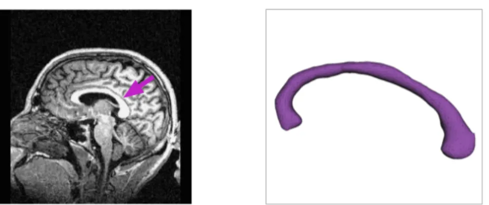
While applications of such tests are still emerging, a few examples can be found in the literature. Kovacev-Nikolic et al. [29] use a statistical test based on persistent homology to detect conformational changes between closed and open forms of the maltose-binding protein. Kwitt et al. [30] use a statistical test to distinguish between demented and non-demented individuals based on MRI of the corpus callosum region of the brain (a study we will refer to throughout the thesis).
Another interesting application would be to use statistical methods to circumvent some of the computational weaknesses of persistent homology. If for instance we consider a large point cloud on which we want to perform Vietoris-Rips filtration, it would be more efficient to repeatedly uniformly subsample from the point cloud, compute persistent homology and average these results, instead of computing the persistent homology of the original point cloud, since the algorithms to compute persistent homology scale poorly. Of course this is only viable if this averaging is possible and can be shown to approximate the result of persistent homology on the original point cloud in a precise statistical sense. Subsampling is explored in [13].
2.3.2 Overview of approaches
A first possible approach is to consider probability distributions on persistence diagrams. This approach was first explored in [34] where the authors establish Fréchet expectations and variances on the space of persistence diagrams. However Fréchet expectations are not unique which makes the development of statistical methods complicated. Such approaches also face challenges to actually compute the Fréchet means. Turner et al. [48] describe an algorithm for computing the Fréchet mean for a particular class of distributions (combinations of Dirac masses on persistence diagrams). In general the development of such approaches is an active research area.
A second approach is to construct maps from the space of persistence diagrams into spaces where statistical concepts are well-founded, e.g. existence of unique expectation and convergence results that allow for construction of confidence intervals, hypothesis
testing, etc... A persistence landscape [8] constitutes such a map into Lp function
spaces, leveraging the theory of probability in Banach spaces to describe e.g. statistical tests.
A third approach is to construct a kernel on the space of persistence diagrams and rely on the theory of kernel embedding of probability distributions to develop statistical methods for persistent homology. The scale-space kernel constructed in this way was introduced in [42] and its statistical properties in the context of kernel embedding of distributions were explored in [30]. Since this kernel is constructed from a feature map into a function space, it has some similarities with the approaches in the previous paragraph (in fact a kernel can be constructed from persistence landscapes, as is done for comparison in [30]). However the theoretical background and statistical methods developed are very different.
Since our approach is inspired by [30], we will devote the next sections to first describe the theory of kernel embedding of distributions after introducing the relevant concepts, and second describe the kernel proposed in the paper.
2.4 Hilbert spaces, RKHS and kernels
2.4.1 Real Hilbert spaces
A real Hilbert space is a real vector space that is equipped with an inner product which is symmetric, bilinear and positive definite. A real Hilbert space is also a complete metric space with respect to the distance induced by its inner product. An example of a real Hilbert space that we will consider in this thesis is the L2 space of real square
integrable functions:
f :R → R s.t. ) ∞
−∞|f(x)|
2dx <∞, (2.12)
with the inner product given by:
⟨f, g⟩ := ) ∞
−∞
f (x)g(x)dx. (2.13)
d(f, g) :=||f − g|| =»⟨f, f⟩ + ⟨g, g⟩ − 2⟨f, g⟩ for f ̸= g. (2.14)
2.4.2 Kernels
A symmetric function on an arbitrary non-empty set X, K : X × X → R is called a positive-definite kernel if:
n " i=1 n " j=1 cicjK(xi, xj)≥ 0, ∀x1, ..., xn ∈ X given n ∈ N, c1, ..., cn∈ R. (2.15)
2.4.3 Reproducing Kernel Hilbert Spaces
For a non-empty arbitrary set X, we consider a Hilbert space H of functions f : X → R. H is said to be a Reproducing Kernel Hilbert Space (RKHS) if there exists an M > 0 s.t.:
|f(x)| ≤ M||f||H,∀f ∈ H. (2.16)
An RKHS has the important property that there exists for each x ∈ X a unique element Kx ∈ H s.t.
f (x) =⟨f, Kx⟩H,∀f ∈ H. (2.17)
In words we can evaluate functions by taking inner products in the RKHS. The reproducing kernel K : X × X → R of H is then defined as K(x, y) = ⟨Kx, Ky⟩H.
The Moore-Aronszajn theorem provides a kind of converse to this since it allows the construction of an RKHS from an arbitrary kernel. Formally: for any kernel K on a set X as defined in2.4.2, there exists an RKHS of functions f : X → R for which K is the reproducing kernel. Starting from a kernel K, we can thus arrive at Kx = K(x,·).
2.5 Kernel embedding of probability distributions
2.5.1 Maximum Mean Discrepancy
We let X be a topological space on which we define two random variables x and y with Borel probability measures p and q respectively (for which we use the shorthand x ∼ p and y ∼ q). We denote Ex[f (x)] := Ex∼p[f (x)] and Ey[f (y)] := Ey∼q[f (y)] the
expectations with respect to p and q respectively. We further let F be a class of functions f :X → R. The Maximum Mean Discrepancy (MMD) is defined as:
MMD[F, p, q] := sup
f∈F
(Ex[f (x)]− Ey[f (y)]). (2.18)
It would now be useful to discover function classes F rich enough for MMD to distinguish probability measures. Formally we want the following to hold:
p = q ⇔ MMD[F, p, q] = 0. (2.19) If further an empirical estimate of MMD can be computed from two samples X and Y drawn from p and q respectively (as will be formalized later on), then this estimate may be used as a test statistic in the context of a test for equality of distributions.
2.5.2 MMD and RKHS
While the space C(X ) of bounded continuous functions on X fulfills the condition2.19
if (X , d) is a metric space [17], we want to discover function classes that will allow us to practically compute the MMD.
To this aim we now let H be an RKHS of functions f : X → R with reproducing kernel k, as defined in 2.4.3. Under some conditions H has the property that a probability distribution p is said to embed in H through its mean map µp ∈ H where µp is such
that Ex[f ] = ⟨f, µp⟩H. This can be thought of as analogue to the reproducing property
of the RKHS, allowing us to compute expectations by evaluating inner products in the RKHS. We now state two equivalent conditions for the existence of µp ∈ H:
1. k(·, ·) is measurable and Ex[
!
k(x, x)] <∞ [24]. 2. k(·, ·) is measurable and bounded on X [45].
We now let F be the space of functions f ∈ H s.t. ||f||H ≤ 1. Assuming the existence
of µp, µq ∈ H as defined above we are able to express:
MMD2[ F, p, q] = + sup f∈F⟨µ p− µq, f⟩H ,2 =||µp− µq||2H
= Ex,x′[k(x, x′)] + Ey,y′[k(y, y′)]− 2Ex,y[k(x, y)],
(2.20)
where x, x′ are independent random variables distributed under p, and y, y′
independent random variables distributed under q. This offers two perspectives on MMD that will prove to be useful: as the distance between mean maps in H, and as an expression involving expectations of the kernel function.
2.5.3 Universality
We further want a criteria to determine if the condition p = q if.f. MMD[F, p, q] = 0 holds for F. This is not the case for all RKHS. For instance if we let X be R and H the space of linear maps f :R → R then MMD[F, p, q] = supa∈R,a≤1[a(E[x]− E[y])], that is it would be sufficient for p and q to have the same mean for MMD[F, p, q] to be 0 (while they may still, for example, have different variances).
There is a class of RKHS, called universal, for which the condition holds if X is a compact metric space. A condition for H to be universal is for the reproducing kernel k(·, ·) to be continuous and for H to be dense in C(X ) with respect to the L∞norm. Another – perhaps more practical – sufficient condition for universality is provided by Christmann and Steinwart [14]. The theorem states that for a compact metric space X , a separable Hilbert space G and a continuous injective map ρ : X → G the following kernel is universal (that is, the RKHS for which kU is the reproducing kernel
is universal): kU(x, x′) := ∞ " n=0 an⟨ρ(x), ρ(x′)⟩nG, for x, x′ ∈ G, an > 0. (2.21)
2.6 Empirical estimates and hypothesis test
2.6.1 Empirical estimates
We now consider a first set X = {xi}mi=1 of observations from a sequence of i.i.d.
random variables distributed under p and a second set of observations Y = {yi}ni=1
from a sequence of i.i.d. random variables distributed under q.
A first empirical estimate can be obtained by replacing µp by m1 -mi=1k(xi,·) and µqby 1
n
-n
i=1k(yi,·) in equation2.20:
MMDb[F, X, Y ] = || 1 m m " i=1 k(xi,·) − 1 n n " i=1 k(yi,·)||H = . 1 m2 m " i,j=1 k(xi, xj) + 1 n2 n " i,j=1 k(yi, yj)− 2 mn m,n " i,j=1 k(xi, yj) /1 2 . (2.22)
While MMDb[F, X, Y ] is the minimum variance estimator [24], it is however biased
(E0MMDb[F, X, Y ]
1
̸= MMD[F, p, q]) due to the inclusion of terms of type k(xi, xi)
and k(yi, yi). Removing these terms and working with an estimate of MMD2 we
obtain: MMD2 u[F, X, Y ] = 1 m(m− 1) m " i=1 m " j̸=i k(xi, xj) + 1 n(n− 1) n " i=1 n " j̸=i k(yi, yj)− 2 mn m,n " i,j=1 k(xi, yj). (2.23) Unbiasedness of MMD2
u[F, X, Y ] follows from the fact that it is a U-statistic [44] (on
the other hand, MMDb[F, X, Y ] is an example of a V-statistic). The choice between
MMDb[F, X, Y ] and MMD2u[F, X, Y ] is thus an example of the bias-variance tradeoff
[20].
Gretton et al. [24] show that both empirical estimates are consistent, that is they converge in probability to the population MMD. Moreover, the convergence rate is shown to be O((m + n)−1
2).
2.6.2 Two-sample hypothesis test
We briefly describe the framework of a two-sample hypothesis test as can be found in [10]. We are in presence of two i.i.d. samples X and Y , drawn from probability distributions p and q respectively. We formulate the two complementary hypotheses:
• H0 : p = q (null hypothesis),
• Ha : p̸= q (alternative hypothesis).
The goal of the two-sample hypothesis test is now to distinguish between the two hypotheses, based on the samples X, Y . This is done by defining a threshold t (delimiting the acceptance region of the test), such that if MMDb[F, X, Y ] < t then
H0is accepted, otherwise rejected. Two kinds of errors can be made: a Type 1 error is
made when p = q is wrongly rejected, while a Type 2 error is made if p = q is wrongly accepted.
While designing the test, a level α is defined, it is an upper bound on the probability of a Type 1 error from which the threshold t is derived. Alternatively a p-value can be computed, which corresponds to the probability, under the null hypothesis, of sampling a test statistic at least as extreme as that which was observed. H0can thus be
rejected if the p-value does not exceed α.
2.6.3 Distribution of test statistic
In order to use MMDb as test statistic in two-sample hypothesis test, the distribution
under the null hypothesis p = q needs to be understood. Gretton et al. derive an acceptance region for a hypothesis test of level α and where K is s.t. 0 ≤ k(x, y) ≤ K and m = |X| = |Y |: MMDb[F, X, Y ] < … 2K m (1 + ! 2 log α−1). (2.24)
This acceptance region may be used for the two-sample hypothesis test. Another alternative, which we will apply in this thesis following [30], is to approximate the distribution of the test statistic under the null hypothesis by bootstrapping on the aggregated data. This procedure is described by Efron and Tibshirani in [18] and for V-statistics in [2]. This distribution is then used to calculate a p-value.
For our samples X and Y such that |X| = n, |Y | = m, we denote the combined sample of X and Y by Z (thus |Z| = n + m). We get the following algorithm:
1. Draw N samples of size n + m with replacement from Z. Call the first n observations X∗and the remaining m observations Y∗.
2. Evaluate MMDb[F, X∗, Y∗] on each sample to obtain MMD(i)b for i = 1, ..., N.
3. Compute the p-value as p = 1 N
-N
i=1I{MMD (i)
b ≥ MMDb[F, X, Y ]} (where I is
the indicator function).
2.7 Scale-space kernel
The scale-space kernel, described in Reininghaus et al. [42], is defined from a feature map Φσ : D → L2(Ω) where D is the space of persistence diagrams (see 2.1.7) and
Ω ⊂ R2 is the closed half-plane above the diagonal. Inspired by scale-space theory
[28], the feature map is the solution to a heat diffusion differential equation, defined by setting as initial conditions a sum of Dirac deltas on the points in the persistence diagram and a Dirichlet boundary condition on the diagonal. Once the feature map is obtained by solving the differential equation, a kernel is defined as the inner product in L2(Ω) and the kernel can be expressed in closed-form for F, G∈ D:
kσ(F, G) :=⟨Φσ(F ), Φσ(G)⟩L2(Ω) = 1 8πσ " p∈F,q∈G e−||p−q||28σ − e−||p−¯ q||2 8σ . (2.25)
The parameter σ can be seen as controlling the scale of the kernel. The points p, q = (s, e) are points of the persistence diagrams and ¯q = (e, s), the point mirrored in the diagonal.
The kernel is shown to be stable with respect to the Wasserstein distance (see 2.1.7) for p = 1. By considering probability distributions on a subset of D on which some conditions are imposed (all points in the diagrams are start/end bounded, as well as the total multiplicity of the diagrams) it is further shown that the RKHS H for which kσ is the reproducing kernel has the property that probability distributions can be
said to embed in H through their mean map (see 2.5.2), justifying the application of statistical methods from the theory of kernel embedding of distributions to the space of persistence diagrams. A kernel derived from kσ and defined as kσU(F, G) :=
exp(kσ(F, G)) is further shown to be universal (see2.5.3).
2.8 Machine learning
2.8.1 Kernel methods
We will briefly introduce kernel methods for machine learning and make the connection to the background on kernels in section 2.4. One way to understand the usefulness of kernels is to start from the formulation of support-vector machines (SVM), a well-known kernel method. If we take the setting of a binary classification, we have a training set {(xi, yi)}Ni=1where xi ∈ Rd1 is a vector of predictors and yi ∈ {0, 1}.
Instead of the original predictors we can choose to work with φ(xi), an arbitrary feature
map φ :Rd1 → Rd2. SVM now proposes to find a decision boundary that is a hyperplane in the feature space (for the formulation of the optimization problem see [20]). Solving the optimization problem, it appears that SVM predicts the class y∗for an out of sample
observation x∗ as: y∗ = sgn( N " i=1 wiyi⟨φ(xi), φ(x∗⟩), (2.26)
where wi are coefficients obtained by solving the optimization problem. Thus the
prediction (and the solution of the optimization problem) only requires inner products in the feature space. This opens up to work with feature maps to an arbitrary Hilbert space H and not just Euclidean, i.e. φ : Rd1 → H, something that will be exploited in this thesis. Further, as any kernel as defined in2.4.2realizes an inner product in some (possibly unknown) Hilbert space, one is not required to construct φ(xi) explicitly, but
can directly construct a kernel k(xi, xj) (satisfying the conditions in 2.4.2) which can
be seen as a similarity function between two observations (this is the so-called kernel trick).
2.8.2 Artificial neural networks
A (feedforward) artificial neural network [23] can be seen as a particular class of statistical models for a conditional probability P (Yi = yi|Θ = θ, Xi = xi) where
and Θ parameters. For instance for a binary classification problem where yi ∈ {−1, 1}
one has:
P (Yi = yi|Θ = θ, Xi = xi) = sigm(yifθ(xi)), (2.27)
where fθ : Rd → R (in the case of binary classification problem for a d-dimensional
input vector) is s.t. fθ = f(n) ◦ ... ◦ f(1), i.e. a composition of functions of type
f(i)(h(i−1)) = g(i)(W(i)h(i−1) + b(i)). We say that f(i) represent transition functions
between layers h(i−1)and h(i)(h(0)being the input layer of the neural network and h(n)
the output layer), W(i), b(i) ⊂ θ are parameters and g(i) is called an activation function
(e.g. ReLu or sigmoid) and is applied component-wise.
For a training set {(xi, yi)}Ni=1(that is, outcomes of {(Xi, Yi)}Ni=1) one typically computes
ˆ
θ by maximum likelihood of P (Yi = yi|Θ = θ, Xi = xi) on the training set
(using the backpropagation algorithm). Predictions for out-of-sample observations are computed based on this estimate of θ.
After this brief introduction we will now focus on aspects of neural networks that will be of particular importance for the models developed in this thesis.
2.8.3 Sets as inputs to neural networks
In the previous section we considered the input of a neural network to be a vector inRd,
which is the general assumption. We will now consider instead neural networks where the input is a set. We can formulate this by first defining a set X . Then the power set 2X is the input domain of our neural network. A point cloud is an example of such an input, where X = Rdand an input X ∈ 2X is thus a set of variable cardinality (though
in practice finite) of points, i.e. vectors inRd. Point clouds are for instance produced
by 3D-scanners.
Formally we can say that our function fθdefined in the previous section for the example
of binary classification is now a function fθ : 2X → R with the property that if
M ∈ N, for any permutation π on {1, ..., M} the following holds: fθ(x1, ..., xM) =
fθ(xπ(1), ..., xπ(M )). We then call fθpermutation-invariant.
While particular forms of permutation-invariant neural networks had been developed, as well as more ad-hoc methods (e.g. adding permuted versions of the data to the
training set, a form of data augmentation), Zaheer et al. [53] proposed a general form for a permutation-invariant network. They show that fθ is permutation-invariant if.f.
it can be decomposed in the form:
fθ(X) = ρ(
"
x∈X
φ(x)), (2.28)
where ρ and φ are suitable transformations. The sum may also be replaced by other permutation-invariant operations (e.g. max, median...). In fact Zaheer et al. only prove this theorem for the case when X is countable (which is not the case for point clouds for instance), but it is conjectured to hold in general.
Hence a general type of architecture for a neural network is defined where from the input layer every member of the set x ∈ X is transformed by φ(x) (possibly through several layers) and this output, for all members of the set, then goes through a permutation-invariant operation such as a sum. There may be several such transformations and their concatenation is then fed into the subsequent part of the network, ρ, which can be defined by several layers.
2.9 Persistent homology and machine learning
2.9.1 Introduction
We now move to investigating the connection between persistent homology and machine learning. In this thesis we will concern ourselves with supervised learning, thus our aim can be seen as developing methods where the information about the topology and geometry of observations in a dataset – as may be extracted with persistent homology – is exploited to attain a lower loss in a particular machine learning problem, for instance classifying observations with high accuracy. While we notice the commonalities between machine learning and statistical methods such as those described earlier (e.g. the analogy between binary classification and statistical tests to distinguish samples from two distributions) we treat them separately and develop different methods (however relying on the same feature map or kernel) in this thesis. While our focus is supervised learning, we note that there are several other interesting intersections between persistent homology and machine learning, which constitute active research areas. One of them is generative models, where persistent
homology may be used to learn representations that are topologically accurate, and less sensitive to adversarial attacks [35]. Another example is topological regularization, where parameters in e.g. a neural network can be forced (or encouraged through priors) to adopt a particular topology, for instance to form clusters [7]. A more specific application of this idea is to encourage connectivity in image segmentation through topological priors [15].
Supervised learning using purely input obtained from the persistent homology method has been shown to be competitive for a few machine learning problems. Within graph learning, when the problem is to classify observations solely based on their graph structure (without any data attached to the edges or vertices) methods based on persistent homology can achieve high accuracy, as is explored in the experiment in section 5.2.2, following [27]. However the most promising route is likely to develop methods that successfully exploit the information extracted by persistent homology as one kind of feature, alongside with other features obtained from the observations in a dataset. It is believed that topological features are often uncorrelated to features that can be extracted through non-topological methods and thus can enhance models in several areas. An illustration of such approach is in Dindin et al. [16] where a neural network is constructed to detect arrhythmia in patients from ECG time series. Persistent homology on the sublevel filtration of the time series (through the use of Betti curves [49]) is used as one input to the neural network, alongside other features derived from the time series. An ablation study is performed, showing that inclusion of topological features increased the accuracy of the classification by several percentage points. It has also been observed [7] that many adversarial attacks in computer vision are of topological nature, which may indicate that convolutional neural networks – which are highly effective at e.g. image recognition – by their strategy of utilizing local connectivity aggregated at higher levels through the convolution operation, may still miss global, topological, characteristics of images.
2.9.2 Overview of approaches
Persistence diagrams, which are typically seen as the topological summaries resulting from persistent homology, do not easily lend themselves to the construction of machine learning methods, due to similar reasons as those discussed in section 2.3.2 and to the fact that a metric structure is generally not enough for the development of
machine learning methods, in which the structure given by Euclidean spaces, or more generally Hilbert spaces, is desirable. In fact, most of the research done to utilize persistent homology in a machine learning context can be seen through this lens: as ways to develop stable mappings with high discriminative power from the space of persistence diagrams to either Euclidean spaces (for neural networks, sometimes called vectorization) or more generally Hilbert spaces (for kernel methods). We will review some of the previous work in those two categories.
A first approach for vectorization is provided by Adams et al. [1] under the name persistence images. For a persistence diagram B rotated clock-wise by π
4, the function ρB :R2 → R is defined as: ρB(z) = " p∈B φp(z)· w(p), (2.29)
where φpis taken to be the Gaussian centered at p, and w is a function that can be used
to weigh areas of the persistence diagram differently. Thus intuitively ρB(z) gives a
measure of the density of points of the persistence diagram in the neighborhood of z. This is further vectorized by fixing a grid and integrating ρB(z) over each square of the
grid.
A first approach for a kernel constructed from a mapping into a Hilbert space is the scale-space kernel [42] described in section2.7.
Persistence Landscapes [8] are defined for a persistence diagram B as piecewise linear functions λB : Z+× R → R. The building block is a ”tent” function λp(t) defined for
each point p = (s, e) of the persistence diagram as:
λp(t) := ⎧ ⎪ ⎪ ⎪ ⎪ ⎨ ⎪ ⎪ ⎪ ⎪ ⎩ t− s if t ∈ [s,s+e 2 ], e− t if t ∈ [s+e 2 , e], 0 otherwise. (2.30)
From this λB(k, t) = kmaxp∈Bλp(t) is defined, where kmax is the k:th largest value in
the set. Persistence landscapes have been applied both for vectorization by discretizing λB(k, t), and as a kernel method: since λBcan be seen as a mapping into L2, a kernel
2.9.3 Learnable parameters
While a mapping from persistence diagrams into function spaces may be injective, as we saw was the case for the the ample stable rank (2.2.4) and for the feature map from which the scale-space kernel (2.7) is derived, the discretization induced by a vectorization (to Rn) will intuitively mean that some data is preserved while
some is lost. A natural question is thus to ask whether this choice can be made explicit. Some methods indeed give some control over this choice by parametrizing the vectorization, as was the case for the persistence images defined in equation
2.29, where the weighing function allowed to incorporate priors over which areas of the diagram are thought to be the most important for a particular task. However, since designing such priors is hard, efforts have recently concentrated on producing vectorizations that are not only parametrizable, but where those parameters can be learned during the training of a neural network. Typically this is done by ensuring that the loss function defined by a neural network is differentiable with respect to the parameters, so that those can be learned during backpropagation together with the other parameters of the network. Such methods can thus claim to provide a task-specific (for a particular learning problem, e.g. for a fixed dataset, loss function and network design) optimal vectorization, that is optimal among the parametrizable family of functions considered.
The first such approach by Hofer et al. [27] has similarities with both the scale-space kernel and persistence images. The building block is a Gaussian-like function Sµ,σ,ν(s, e) applied on a point (s, e) of a persistence diagram B rotated clock-wise by π4,
where ν is fixed but the parameters µ = (µ0, µ1) and σ = (σ0, σ1) are designed to be
learned during the training phase. It is defined as:
Sµ,σ,ν(s, e) := ⎧ ⎪ ⎪ ⎪ ⎪ ⎨ ⎪ ⎪ ⎪ ⎪ ⎩ exp {−σ2 0(s− µ0)2− σ21(e− µ1)2} if e ∈ [ν, ∞), exp {−σ2 0(s− µ0)2− σ21(lneν + ν− µ1) 2} if e ∈ (0, ν), 0 if e = 0. (2.31)
From this building block, a vectorization (into R) is obtained for B by summing over all points in the persistence diagram: -(s,e)∈BSµ,σ,ν(s, e). This function being
differentiable with respect to µ and σ, it can serve as the first layer of a neural network. For a richer representation, n pairs of parameters (µ, σ) can be initialized, leading to
a learnable representation as a fixed-size vectorRn. A follow-up paper [26] considers
other building blocks, which may have better numerical stability properties than the Gaussian-like one.
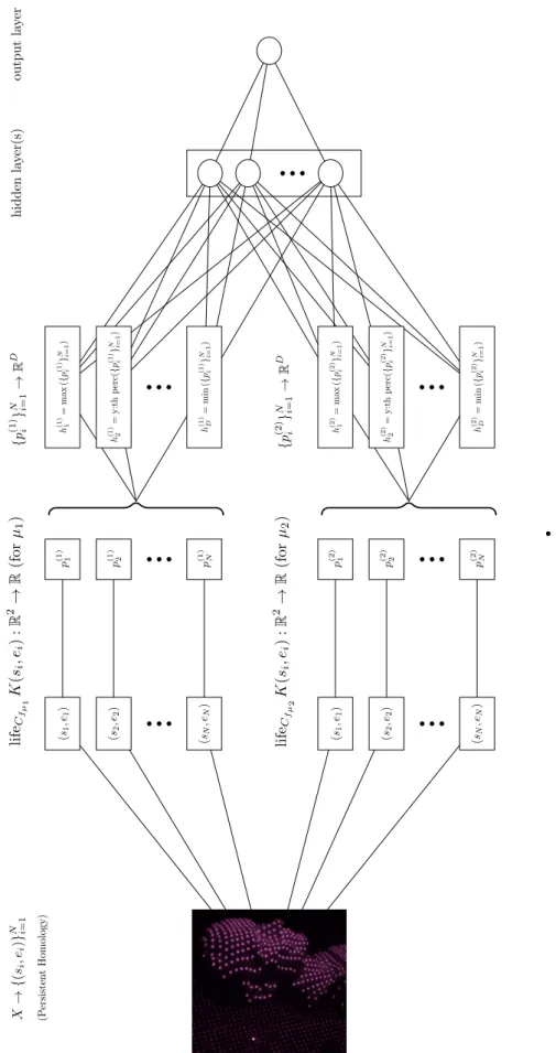
Learnable representations are further generalized in PersLay [9], which inspired by permutation-invariant networks [53] described in section2.8.3, defines a generic form for an input layer of a neural network as:
PERSLAY(B) := op({w(p) · φ(p)}p∈B), (2.32)
where op is a permutation-invariant operation (such as sum, max, etc...), w is a weighing function (such as the one defined for persistence images) and φ is a parametrizable function which maps each point of the diagram into a vector. For instance for the construction above φ = Sµ,σ,ν, op is the sum operation, and w(p) = 1.
2.9.4 Stability
Most mappings are constructed to be stable, that is they have a Lipschitz property, which was seen for example for stable rank (2.2.3). This quest can also be seen in the construction by Hofer et al. described in equation2.31, where the transformation of points within a fixed distance ν of the diagonal is necessary to fulfill Lipschitz-continuity with respect to the Wasserstein metric on the space of persistence diagrams with p = 1. Such transformations, which lead to points of low persistence being discounted compared to other points, corresponds to a prior of considering such points as noise, or at least of less importance for learning problems. This is however not true in general, as commented on in [11].
Kernel-based learning and statistical
analysis
3.1 Introduction
In this section we will define kernels based on stable rank, and describe how they can be used in the context of kernel methods in machine learning. We then proceed to describe the reproducing kernel Hilbert space (RKHS) that can be derived from the kernels and show that they have the property that probability measures on the underlying space of tame parametrized vector spaces can be said to embed in this RKHS. We will examine some of the properties of the kernels such as universality. Finally we will describe a two-sample hypothesis test based on the kernels.
The methodology borrows from Reininghaus et al. [42] and Kwitt et al. [30] in that the goal is to develop first a kernel, second a statistical method for persistent homology using kernel embedding of distributions. The kernels are however constructed in different ways since they are based on different feature maps. This construction needs to be described and mathematically motivated, which is the goal of this section. Once established, the computational and discriminative properties can be examined, with the hope of providing an alternative to the method based on the kernel described in the two cited papers, and in general to other machine learning and statistical methods based on persistent homology.
3.2 Restrictions on parametrized vector spaces
We consider Tame([0, ∞), Vect), the collection of tame, [0, ∞)-parametrized vector spaces, as defined in2.1.5. We further consider a fixed contour C of distance type (as defined in2.2.1). We now define TameT,N([0,∞), Vect) as the collection of elements
V ∈ Tame([0, ∞), Vect) where V is s.t:
1. There is a T ∈ [0, ∞) such that Va= 0 for all a > T .
2. rank(V ) ≤ N (N ∈ N).
3.3 Interpretation of the restrictions
While imposing such bounds is necessary for the theoretical development, they do not in practice constitute limitations. To illustrate this, we consider applying Vietoris-Rips on a point cloud, i.e. a finite metric space (X, d) with |X| = M points. Such point cloud has2M
2
3
pairwise distances, which could be ordered to obtain a sequence d1, ..., d(M
2) such that di ≤ di+1. d( M
2) is thus the maximum distance between any two points, called the diameter of the point cloud. From the definition of Vietoris-Rips
(see 2.1.4) VRt(X, d) = VRv(X, d) for d(M
2) ≤ t ≤ v, and taking the corresponding tame parametrized vector space V , Vt≤vis an isomorphism. If necessary, one can thus
without loosing any information ”truncate” V by setting Vv = 0 and Vt≤v be the map
from Vtto 0, for t < d(M 2) ≤ v.
We also see that for di ≤ t ≤ v < di+1 we have VRt(X, d) = VRv(X, d). Thus the
minimal discretizing sequence (see2.1.5) τ of V must be such that |τ| ≤ 2M 2
3
. By the definition of the rank of V in terms of dimension of direct sums of cokernels (2.2.3) we must have rank(V ) ≤ dim(Vd1) + ... + dim(Vd
(M 2)
). Recalling the definition of homology
from2.1.3we can further find a bound on dim(Vt) based on the number of n-simplices,
e.g. for H0homology the bound is the maximum number of 0-simplices, i.e. M. Hence
the rank in that case is bounded by M ·2M 2
3 . One can further consider M and d(M
2) derived from e.g. storage capacity of computers and not from a particular dataset.
3.4 Constructing the kernels
For a chosen contour C we will construct two kernels: K1
C and KC2. We do this by first
showing that Ÿ!rankC(V ) and rankC(V ) (defined in2.2.3and2.2.4) are square-integrable
for V ∈ TameT,N([0,∞), Vect). We then define the kernels as inner-products in L2(L2
was defined as an example of a Hilbert space in2.4). The references to e.g. definitions and propositions in the following proofs are found in [11].
Proposition 2. Ÿ!rankC(V )⊂ L2(R) for V ∈ TameT,N([0,∞), Vect).
Proof. By Definition 2.1 Ÿ!rankC(V ) is a Lebesgue-measurable function [0,∞) → [0, ∞).
We need to show that Ÿ!rankC(V ) is square-integrable. By Definition 7.1, Ÿ!rankC(V ) is
a non-increasing piecewise constant function. It is bounded because ¤!rankC(V )(0) =
rank(V ) ≤ N by Corollary 7.9 and condition 2 in3.2(we note however that this holds even without the bound on the rank since the rank is finite for any tame parametrized vector space). Since Ÿ!rankC(V ) is a piecewise constant function, requiring it to be
square-integrable is equivalent to requiring it to have bounded support (for otherwise limt→∞rank¤!C(V )(t) > 0 and it can not be square-integrable).
We consider the decomposition of V as ⊕n
i=1K(si, ei). From condition 1 in 3.2 we
know that ei ≤ T , ∀i. Following Proposition 8.2 we have that lifeCK(si, ei) =
C(si,−)−1(ei). From the properties of regular contours stated in2.2.1 we must have
that lifeCK(si, ei) = C(si,−)−1(ei) ≤ C(0, −)−1(T ). For otherwise assume Li =
C(si,−)−1(ei) > C(0,−)−1(T ) = LT. Then ei = C(si, Li) > C(0, LT) = T (by
Definition 1 (si, Li) ≥ C(0, LT) but since the contour is regular C(−, ϵ) and C(a, −)
are mononorphisms hence (si, Li) > C(0, LT)) which contradicts condition 1 in 3.2.
We define ℓmax = C(0,−)−1(T ).
From what we established and Corollary 8.3 we have that ¤!rankC(V )(t) = 0 for t > ℓmax.
Thus Ÿ!rankC(V ) is square-integrable.
Proposition 3. rankC(V )⊂ L2(R2) for V ∈ TameT,N([0,∞), Vect) and α ∈ [0, T ].
Proof. In 2.2.4 we saw that rankC(V ) is such that for a fixed α, rankCf(V )(t, α) = ¤!
It holds for α ≤ T that lifeC/α(si, ei) ≤ lifeC(si, ei) (Proposition 8.2). For a fixed α we
thus have that rankC(V ) has finite support [0, ℓmax] and is therefore square-integrable.
Since we consider α ∈ [0, T ], it thus holds that rankC(V )(t, α) is bounded, has
finite support [0, ℓmax] × [0, T ] and is therefore square-integrable, i.e. an element of
L2(R2).
Proposition 4. K1
C, KC2 : TameT,N([0,∞), Vect)×TameT,N([0,∞), Vect) → R defined
by: • K1 C(V, W ) := *∞ 0 rank¤!C(V )(t) ¤!rankC(W )(t)dt, • K2 C(V, W ) := *T 0 ( *∞ 0 rankC(V )(t, α) rankC(W )(t, α)dt)dα,
are kernels as defined in2.4.2.
Proof. The functions are by definition inner products in the Hilbert space L2 of the
feature maps of two elements in TameT,N([0,∞), Vect). Any inner product is symmetric
and positive-definite.
3.5 Stability of the kernels
3.5.1 First kernel
Using the definition in 2.4.1, the norm derived from the inner product in L2
induces a pseudometric on f, g ∈ L2, hence on Ÿ!rank
C(V ), ⁄!rankC(W ) for V, W ∈
TameT,N([0,∞), Vect), called the L2-distance:
dL2( Ÿ!rankC(V ), ⁄!rankC(W )) = ( ) ∞ 0 | ¤! rankC(V )(t)− ¤!rankC(W )(t)|2dt) 1 2. (3.1)
Proposition 2.2 [11] establishes the following stability result:
dL2( Ÿ!rankC(V ), ⁄!rankC(W ))≤ c dC(V, W ) 1
2, (3.2)
where dC is the pseudometric on Tame([0, ∞), Vect) with respect to the contour C as