SKI Report 01:27
Research and Development Program in
Reactor Diagnostics and Monitoring with
Neutron Noise Methods
Stage 7. Final Report
I. Pázsit
C. Demazière
V. Arzhanov
N.S. Garis
August 2001
Research
SKI PERSPECTIVE
How this project has contributed to SKI’s research goals
The overall goals for SKI research are:
• to give a basis for SKI ’s supervision
• to maintain and develop the competence and research capacity within areas
which are important to reactor safety
• to contribute directly to the Swedish safety work.
Above all, this project has contributed to the strategical research goal of competence and research capacity by building up competence within the
Department of Reactor Physics at Chalmers University of Technology regarding reactor physics, reactor dynamics and noise diagnostics. The project has also contributed to the research goal of giving a basis for SKI’s supervision by developing methods for identification and localization of perturbations in reactor cores.
The report comprises stage 7 of a long-term research and development program. The results have been published in international journals and have been included in both licentiate- and doctor’s degrees.
Project information:
Project manager: Ninos Garis, Department of Reactor Technology, SKI
Project number: 14.5-000983-00156
Previous reports: SKI report 95:14 (1995), 96:50 (1996), 97:31 (1997), 98:25 (1998), 99:33 (1999), 00:28 (2000).
SKI Report 01:27
Research and Development Program in
Reactor Diagnostics and Monitoring with
Neutron Noise Methods
Stage 7. Final Report
I. Pázsit¹
C. Demazière¹
V. Arzhanov¹
N. S. Garis²
¹Chalmers University of Technology, Department of Reactor Physics,
412 96 Gothenburg
²Swedish Nuclear Power Inspectorate (SKI),
106 58 Stockholm
August 2001
This report concerns a study which has been conducted for the Swedish Nuclear Power Inspectorate (SKI). The conclusions and viewpoints presented in the report are
Research
Research and Development Program in Reactor Diagnostics
and Monitoring with Neutron Noise Methods: Stage 7
Summary
This report gives an account of the work performed by the Department of Reactor Physics, Chalmers University of Technology, in the frame of a research contract with the Swedish Nuclear Power Inspectorate (SKI), contract No. 14.5-000983-00156. The present report is based on work performed by Imre Pázsit (project leader), Christophe Demazière, Vasiliy Arzhanov and Ninos Garis, SKI.
This report constitutes stage 7 of a long-term research and development program concerning the development of diagnostics and monitoring methods for nuclear reactors. The long-term goals are elaborated in more detail in e.g. the Final Reports of stage 1 and 2 (SKI Rapport 95:14 and 96:50, Refs. [1] and [2]). Results up to stage 6 were reported in [1] - [6]. A proposal for the continuation of this program in stage 8 is also given at the end of the report.
The program executed in stage 7 consists of three parts and the work performed in each part is summarized below.
Development of a 2-D 2-group neutron noise simulator
In stage 6, the basic principles of a 3-D fully coupled neutronic/thermal-hydraulic simulator in the frequency domain were presented. The neutronic model relied on the two-group diffusion approximation, whereas the thermal-hydraulic algorithms relied on the so-called “lumped” model. The key element of this simulator was that only the static data were required which could be obtained from the Studsvik Scandpower CASMO-4/TABLES-3/ SIMULATE-3 code package.
The simulator was developed with this underlying idea, which means that the calculation of the static fluxes and the eigenvalue were avoided. Depending on what kind of spatial discretization scheme which is used in the noise simulator to calculate the “leakage” noise, it is not granted that the system remains critical by using the group constants supplied by SIMULATE. Nevertheless, when the system is critical, the balance equations should be fulfilled in all nodes with respect to the discretization scheme used. In concrete terms, the calculation of the static fluxes and eigenvalue can be avoided if the system is brought back to criticality by modifying the cross-sections so that the balance equations are always fulfilled with the chosen spatial discretization scheme.
This approach was used in this study with the finite difference scheme. As pointed out in stage 6, the finite difference scheme is relatively inefficient compared to finite elements or nodal methods, but on the other hand it is rather easy to implement. These two more sophisticated schemes are planned to be investigated at a later stage, but for the time being the simulator relying on the finite difference scheme was improved as much as possible so that a 2-D entirely neutronic model could be used for routine calculations. Such a simplified model has plenty of applications, both theoretical and practical ones.
Therefore, much emphasis was put in this stage on the calculational efficiency of the noise simulator. The CPUtime was reduced by a factor 15 and the required memory by a factor 8, compared to the previous version. Benchmarking of this noise simulator showed that the level of accuracy on the flux noise (both its amplitude and its phase) is excellent for
all noise source types. However, these comparisons were made for homogeneous systems since these are the only systems for which analytical solutions can be determined. It is expected that the accuracy could deteriorate for heterogeneous systems. Thus a need remains to use a more efficient spatial discretization scheme than the finite difference one.
Application of the neutron noise simulator to anomaly localisation
The 2-D 2-group noise simulator calculates the neutron noise induced by any type of noise source, spatially distributed or not (i.e. localised). It can also be used in an inversion task; the neutron noise can be used as input parameter to an algorithm which determines the location of the corresponding noise source. Such a localisation task was previously developed by Karlsson and Pázsit ([14], [15]).
In this stage, the localisation algorithm was improved since the 2-D 2-group neutron noise simulator was used for the calculation of the transfer function, as opposed to the transfer function corresponding to a homogeneous system as in [14] and [15]. At that time, this means that any realistic core can be studied via this algorithm. It was shown, through simulations, that the localisation procedure located the noise source successfully as long as only one noise source existed in the core. If several noise sources are present simultaneously, selecting a few detectors around a region where one of the noise sources is assumed to be found allows locating this specific noise source properly. Another interesting feature of this improved localisation procedure is that the algorithm is less sensitive to the extraneous background noise, probably due to the fact that the removal cross-section noise to neutron noise transfer function was used in the noise simulator. This was not possible to perform in the previous algorithm that only used one-group theory.
Finally, the localisation algorithm was applied to the Forsmark 1 channel instability event monitored in January 1997 during fuel cycle 16. By selecting a proper set of detectors, the noise source was located close to a fuel element that was discovered to be unseated. Nevertheless, selecting different detector combinations give also sometimes different results, which suggests that there were several simultaneous noise sources in the Forsmark 1 case.
Wavelet analysis of Oskarshamn 2 data for detector tube impacting
Detection of impacting of detector tubes, also called instrument strings, have been a matter of interest both in Swedish and foreign BWRs. Although detection of the vibrations is relatively simple, the discovery and quantification of the severity of impacting is far more complicated. No single method exists that gives absolute results without calibration or comparison with reference measurements.
Most known methods, frequently applied in the past require comparison with a reference, i.e. impacting-free state, such as the broadening of the peak, decreasing of the decay ratio, or distortion of the probability distribution function. However, some time ago wavelet analysis was tried to detect and quantify impacting on an absolute basis, i.e. without the need for calibration ([3], [23]). In that early work a simple wavelet, the Haar wavelet transform was used. The objective of the recent research was to continue this work with two extensions. The first was to test the method on measurements, taken in Oskarshamn 2 during three fuel cycles by GSE Power Systems AB. For these measurements, damage of some vibrating tubes was registered during refuelling. Thus, these data lend an excellent possibility to test any method for detecting impacting. The
second extension was to test other wavelet transforms than the Haar wavelet, to see if there exists a waveform that is more effective in the detection of impacting.
Due to the large amount of data to be processed, in this stage only the first extension could be investigated. A thorough investigation of all measurements was made with the Haar wavelet method. This report gives a complete presentation of these investigations. A good correlation was found between the most severely impacting tubes and the wavelet results. The extension of the investigations to other wavelet forms was left to the next stage.
Forskningsprogram angående härddiagnostik
och härdövervakning med neutronbrusmetoder: Etapp 7
Sammanfattning
Denna rapport redovisar det arbete som utförts inom ramen för ett forskningskontrakt
mellan Avdelningen för Reaktorfysik, Chalmers tekniska högskola och Statens
Kärnkraftinspektion (SKI), kontrakt Nr. 14.5-000983-00156. Rapporten är baserad på arbetsinsatser av Imre Pázsit (projektledare), Christophe Demazière, Vasiliy Arzhanov och Ninos Garis (SKI).
Rapporten omfattar etapp 7 i ett långsiktigt forsknings- och utvecklingsprogram angående utveckling av diagnostik och övervakningsmetoder för kärnkraftreaktorer. De långsiktiga målen med programmet har utarbetats i slutrapporterna för etapp 1 och 2 (SKI Rapport 95:14 och 96:50, Ref. [1] och [2]). Uppnådda resultat fram till etapp 6 har redovisats i referenserna [1] - [6]. Ett förslag till fortsättning av programmet i etapp 8 redovisas i slutet av rapporten.
Det utförda forskningsarbetet i etapp 7 består av tre olika delar och arbetet i varje del sammanfattas nedan.
Utveckling av en 2-D 2-grupp neutronbrussimulator
I etapp 6 utarbetades grundprinciperna för en tredimensionell simulator i
frekvensdomänen med full koppling mellan neutronik/termohydraulik. Neutronmodellen var baserad på tvågrupps-diffusions approximationen, medan de termohydrauliska algoritmerna använde sig av den så kallade “lumped” modellen. En viktig egenskap för denna simulator var enbart statiska värden behövdes som indata, vilka kunde erhållas från koderna CASMO-4/TABLES-3/SIMULATE-3 från Studsvik Scandpower.
Simulatorn utvecklades med beaktande av denna idé, vilket i princip betydde att simulatorn inte behövde användas för att beräkna de statiska flödestätheterna och egenvärdena. Å andra sidan, beroende på vilket diskretiseringsschema man använder i simulatorn för att hantera utläckage, är det inte garanterat att systemet förblir kritiskt med detta förfarande om man använder gruppkonstanterna från SIMULATE i brussimulatorn. Kriticitet hos det statiska systemet i brussimulatorn är mycket viktigt för en korrekt
beskrivning av dynamik vid låga frekvenser. När systemet är kritiskt, måste
balansekvationerna vara uppfyllda i alla noder enligt det diskretiseringsschema som används. I synnerhet kan beräkning av de statiska flödestätheterna och egenvärdet undvikas om systemet återföres till kriticitet genom en modifiering av tvärsnitten så att balansekvationerna i diskretiseringsschemat är uppfyllda.
Denna metod användes i den föreliggande studien med finitdifferensschemat. Som påpekades i etapp 6 är finitdifferensschemat relativt ineffektivt jämfört med finita element metoden eller med de nodala metoderna; å andra sidan är det enkelt att implementera. Vi planerar att undersöka de ovannämnda två mera komplicerade scheman i ett senare skede, men för närvarande har vi förbättrat finitdifferensschemat så mycket som möjligt så att en
tvådimensionell, enbart neutronbaserad, modell kunde användas för rutinmässiga
beräkningar. En sådan, någorlunda enkel, modell kan användas för ett stort antal potentiella tillämpningar, både teoretiska och praktiska.
Följaktligen har vi lagt ner mycket arbete i denna etapp på den beräkningsmässiga effektiviteten av brussimulatorn. Snabbheten ökades med en faktor 15, och minnesåtgången
minskades med en faktor 8, jämfört med den föregående versionen. Ett test av denna brussimulator visade att noggrannheten i beräkningen för såväl amplitud som fas hos bruset är utmärkt oavsett typ av bruskälla. Dessa tester utfördes för homogena system, eftersom analytiska lösningar enbart kan erhållas för sådana fall. Man kan förvänta sig att noggrannheten skulle kunna försämras för heterogena system. Detta betyder samtidigt att det kvarstår ett behov av att använda ett mer effektivt rums-diskretiseringsschema än finita differens metoden.
Tillämpning av brussimulatorn för lokalisering av en anomali
Brussimulatorn beräknar neutronbruset i två dimensioner med tvågruppsteori, framkallad av en bruskälla med en i princip godtycklig rumsfördelning. Den kan även användas i en så kallad invers uppgift, nämligen i en algoritm som använder neutronbruset
som indata och bestämmer positionen av en lokaliserad bruskälla. En sådan
lokaliseringsalgoritm har utarbetats tidigare av Karlsson och Pázsit ([14], [15]).
I föreliggande etapp har denna lokaliseringsalgoritm förbättrats i och med att D 2-grupps brussimulatorn har använts för beräkning av överföringsfunktionen mellan bruskälla och neutronbrus, till skillnad från överföringsfunktionen motsvarande ett homogent system och engruppsteori som det var fallet i [14] och [15]. Detta betyder samtidigt att den nuvarande algoritmen kan användas även för beräkning av realistiska härdar. Genom simuleringar har vi visat att algoritmen lokaliserar bruskällan korrekt så länge det enbart finns en bruskälla i härden. Om flera lokal bruskällor är aktiva samtidigt, kan man lokalisera varje bruskälla separat genom att använda signaler från ett fåtal detektorer som förmodas omge bruskällan ifråga, istället för att använda alla detektorsignaler. En annan intressant egenskap hos den förbättrade algoritmen är att den är avsevärt mindre känslig för störningar såsom bakgrundsbrus. Anledningen är att i den nuvarande proceduren utgörs bruskällan av fluktuationer av svinn-tvärsnittet, vilka leder till en större lokal komponent än i bruset orsakat av fluktuationer av absorptionstvärsnittet. I den tidigare algoritmen gick det inte använda removalstvärsnittet eftersom den var baserad på engruppsteori.
Slutligen har lokaliseringsalgoritmen använts för lokalisering av kanalinstabiliteten som uppstod i Forsmark 1 i januari 1997 under bränslecykel 16. Genom att välja ett lämpligt antal detektorer har bruskällan (kanalinstabiliteten) lokaliserats i närheten av en bränslepatron som befanns vara osätad under påföljande revision. Emellertid gav val av andra detektorer annorlunda resultat, vilket gör det sannolikt att det fanns flera aktiva bruskällor samtidigt i Forsmark 1 fallet.
Wavelet analys av Oskarshamn 2 data för upptäckt av nötning från vibrerande detektorsonder
Fenomenet med mekaniska stötar (impacting) av detektorsonder mot bränsleboxar har varit föremål för undersökningar både i svenska och utländska kokvattenreaktorer. Medan upptäckt av sondvibrationer är relativt enkelt, är upptäckt och kvantifiering av stötar avsevärt mer komplicerat. Det finns inte någon enskild metod som ger resultat i absoluta termer, utan existerande metoder behöver kalibreras eller jämföras med referensmätningar.
De flesta kända metoderna som hittills har tillämpats kräver jämförelse med en referens, dvs mätdata från vibrationer utan stötar. Metoderna omfattar breddning av
vibrationstoppen i effektspectra, minskning av dämpkvoten, eller en förändring
waveletsanalys prövats för upptäckt och kvantifiering av stötar på ett absolut sätt, dvs utan behov av kalibrering ([3], [23]). I detta tidigare arbete har vi använt en enkel typ av wavelet, den så kallade Haar wavelet transformen. Målet med föreliggande arbete har varit en fortsättning och utvidgning av dessa undersökningar inom två områden. För det första kan metoden testas på mätningar gjorda i Oskarshamn 2 under tre bränslecykler av GSE Power Systems AB. Till dessa mätningar har man även registrerat skador och nötning av vissa sonder under revisionerna. Därmed ger dessa mätdata en utmärkt möjlighet för att testa olika algoritmer för upptäckt av mekaniska stötar. För det andra kan man testa även andra typer av wavelet transform än Haar-transformen, för att undersöka om det finns andra typer som är mer effektiva för upptäckt av mekanisk påverkan.
P g a den stora mängden data, har vi i denna etapp enbart kunnat genomföra den första av de två ovannämnda utvidgningarna av wavelet-metoden. Detta betyder att vi har genomfört en omfattande undersökning av alla mätningar från Oskarshamn 2 med Haar-metoden. Denna rapport ger en fullständig beskrivning av dessa undersökningar. För de sonder som har varit mest utsatta för stötar har vi hittat en bra överensstämmelse mellan waveletanalysens resultat och de verkliga skador som man observerat vid inspektionerna. Utvidgningen av undersökningarna till andra typ av wavelet lämnats till nästa etapp.
Section 1
Development of a 2-D 2-group neutron noise simulator 1.1 Introduction
In stage 6, a 2-group neutron noise simulator, based on the diffusion approximation, was presented [6]. This neutron simulator included also a thermal-hydraulic model, the so-called lumped model, which allowed taking both the fuel temperature and the coolant temperature noise into account. The main advantage of the simulator was its ability to handle any realistic core, since all the necessary data were the static data that could be obtained by using the CASMO-4/TABLES-3/SIMULATE-3 code package from Studsvik Scandpower ([7] - [9]).
The aim of the previous study was to prove that elaboration of such a coupled neutronic/thermal-hydraulic noise simulator was possible, and to highlight the most important features of the code. Nevertheless, it appeared that the spatial discretization scheme used in that study, the so-called finite difference scheme, was not very well adapted to the 3-D calculations of a heterogeneous core. The reason is obviously the relatively poor accuracy of the finite difference scheme for heterogeneous systems when the number of nodes is not too large. Increasing the number of nodes would allow coping with this problem, but the calculational time would unfortunately become prohibitively large. Consequently, it was concluded that using a more sophisticated calculational scheme than the finite difference one was required. The Reactor Physics Department, Chalmers University of Technology has now access to FEMLAB, a multiphysics code based on the finite elements method ([10] and [11]), and plans to study the possibility of using it for the neutron noise simulator. Nodal methods are also considered.
Although the use of a more efficient discretization scheme appears to be absolutely necessary, it was decided to develop a somehow simplified model of the neutron noise simulator for very specific qualitative tasks. In this model (still relying on the finite difference scheme), only the neutronic model is used and the user is able to estimate the corresponding flux noise from any noise source located in the core. All the user needs to do is to define a set of cross-sections, representative of the core, and define the location, strength, and types of noise sources present in the core. Such a qualitative model could already have many practical applications, such as the localisation of anomalies in a reactor from the detector readings (see Section 2), or more theoretical applications such as the evaluation of the Moderator Temperature Coefficient (MTC) of reactivity assuming different shapes/strengths/correlations of the noise sources.
Therefore, the previous simplified model was significantly improved regarding its calculational efficiency and its ease to use. In the following, the neutronic model of the simulator is described in more detail compared to the previous report (see [6]) and benchmarked for different kinds of noise sources.
1.2 Neutron noise simulator
The neutronic model of the noise simulator relies on the two-group diffusion approximation. All calculations are performed in the frequency domain directly, which is equivalent to define complex cross-sections. The main advantages of using the frequency domain instead of the time domain are twofold. First, it is common practice to use the
Fourier transform of the measured signals. Second, because of the Fourier transform, the time derivative in the equations is eliminated. There is consequently no need to properly choose a time discretization which allows taking into account the phenomena one wants to study, and for which the neutron noise has to be evaluated at each time step. In the frequency domain instead, the calculation needs only to be performed once, assuming that the frequency of interest is known. If not, scanning a frequency range does not appear to be a big burden. Finally, the spatial discretization is carried out by using a finite difference scheme.
Neutron noise in the 2-group diffusion approximation
In the two-group diffusion approximation, the time- and space-dependent flux can be expressed as follows:
(1)
and
(2)
with the precursor density given as:
(3)
Assuming that all the time-dependent parameters can be expressed as:
(4) where the index 0 represents the static case, substracting the static case to Eqs. (1)-(3), performing a temporal Fourier transform and neglecting the second-order terms lead to the following matrix formulation:
(5)
where the different matrices are given as: 1 v1 ---∂φ1 t ∂ ---(r t, ) D1(r t, )∇2φ1(r t, ) νΣf 2, (r t, )(1–βeff)φ2(r t, ) λC r t( , ) νΣf 1, (r t, )(1–βeff) Σ– a 1, (r t, )–Σrem(r t, ) [ ]φ1(r t, ) + + + = 1 v2 ---∂φ2 t ∂ ---(r t, ) = D2(r t, )∇2φ2(r t, ) Σ– a 2, (r t, )φ2(r t, ) Σ+ rem(r t, )φ1(r t, ) C ∂ t ∂ ---(r t, ) = βeff[νΣf 1, (r t, )φ1(r t, ) νΣ+ f 2, (r t, )φ2(r t, )] λ– C r t( , ) X r t( , ) = X0( ) δr + X r t( , ) D r( )∇2+φ(r,ω) ( ) δφ1(r,ω) δφ2(r,ω) Σrem( )δΣr rem(r,ω) Σa( )r δΣa 1, (r,ω) δΣa 2, (r,ω) +Σf(r,ω) δνΣf 1, (r,ω) δνΣf 2, (r,ω) + =
(6)
(7)
(8)
(9)
(10)
and the different coefficients are defined as:
(11)
(12)
(13)
From Eq. (5), it is obvious that the right-hand-side represents the neutron noise source. Compared to the calculation of the static neutron flux (which is an eigenvalue problem), the estimation of the neutron noise is a simpler task since there is no need to iterate on the fission term. The only difficulty lies with the fact that Eq. (5) uses complex cross-sections, as the ones defined by Eqs. (11)-(13). These cross-sections are frequency-dependent. This means that a new set of calculation has to be performed for each frequency that one might consider.
2-D spatial discretization
Due to the operator in Eq. (5), a spatial discretization scheme has to be chosen. The finite difference scheme was retained for its simplicity and its efficiency. As will be shown in §1.3, this scheme is satisfactory for homogeneous systems. Nevertheless, it is known that the number of nodes needs to be increased significantly in heterogeneous systems, if one wants to obtain an acceptable level of accuracy. Therefore, other more powerful
D r( ) D1( )r 0 0 D2( )r = φ(r,ω) –Σ1(r,ω) νΣf 2, (r,ω) Σrem 0, ( ) Σr – a 2, (r,ω) = Σrem( )r φ1 0, ( )r φ – 1 0, ( )r = Σa( )r φ1 0, ( )r 0 0 φ2 0, ( )r = Σf(r,ω) φ1 0, ( )r 1 iωβeff iω λ+ ---– – φ2 0, ( )r 1 iωβeff iω λ+ ---– – 0 0 = Σ1(r,ω) Σa 1 0, , ( )r iω v1 --- Σrem 0, ( ) νΣr f 1 0, , ( )r 1 iωβeff iω λ+ ---– – + + = νΣf 2, (r,ω) νΣf 2 0, , ( )r 1 iωβeff iω λ+ ---– = Σa 2, (r,ω) Σa 2 0, , ( )r iω v2 ---+ = ∇2
discretization schemes, such as nodal methods or finite elements, will be considered at a later stage.
The starting point of the discretization procedure is the integration of Eq. (5) over an elementary volume. The unknowns are thus expressed by the following generic formulation:
(14)
whereby the elements of the matrices satisfy the following relationship:
(15)
This way of averaging is consistent with the two-group constants provided by any static core calculator, so that the actual reaction rates are preserved.
If one represents a node I,J by the system of axes and numbering as shown in Fig. 1, the spatial discretization of the neutron noise can be carried out according to the “box-scheme” that allows writing [12]:
(16)
For each direction (either the x or y direction), two expressions for the current noise
can be written by considering the node I,J and its neighbours (either the I+1,J or I,J+1 node respectively). Equating these two expressions allows eliminating the flux noise at the boundary of the two nodes, so that the current noise can be expressed as directly depending on the node-average flux noise in the node I,J and the node-average flux noise in its neighbouring nodes. In a given energy-group g, one obtains:
(17) δXI J, ( )ω ∆ 1 x⋅∆y --- δX r( ,ω)dr I J, (
∫
) = mI J, ( )δω XI J, ( )ω ∆ 1 x⋅∆y --- m r( ,ω)δX r( ,ω)d r mI J, ( )ω ⇔ I J, (∫
) m r( ,ω)δX r( ,ω)dr I J, (∫
) δX r( ,ω)dr I J, (∫
) ---= = 1 ∆x⋅∆y --- D∆δφ∇2δφ(r,ω)dr I J, (∫
) δJI Jx, ( ) δω – JxI–1,J( )ω [ ] ∆x ---– δJI J, y ( ) δω JI Jy, –1( )ω – [ ] ∆y ---– = δJ( )ω δJg I Jx, , ( ) δω – Jg Ix, –1,J( )ω ag I Jx, , δφg I J, , ( )ω +bg I Jx, , δφg I, +1,J( )ω +cg I Jx, , δφg I, –1,J( )ω =(18)
The different coefficients , , , , , and are
summarised in Table I and Table II for the x and y directions, respectively.
Table I. Coupling coefficients in the x direction.
if the node I-1 does not exist 0 if the nodes I-1 and I+1 both exist if the node I+1 does not exist 0 δJI Jy, ( )ω δJI Jy, –1( )ω δJIx–1,J( )ω δJI Jx, ( )ω x y where P x( I,yJ) P
Fig. 1. Principles and convention used in the discretisation scheme (2-D case).
δJg I Jy, , ( ) δω – Jg I Jy, , –1( )ω ag I Jy, , δφg I J, , ( )ω +bg I Jy, , δφg I J, , +1( )ω +cg I Jy, , δφg I J, , –1( )ω = ag I Jx, , ag I Jy, , bg I Jx, , bg I Jy, , cg I Jx, , cg I Jy, , ag I Jx, , bg I Jx, , cg I Jx, , 2 Dg I J, , Dg I, +1 J, ∆x D( g I J, , +Dg I, +1 J, ) ---2 Dg I J, , ∆x ---+ 2 Dg I J, , Dg I, +1 J, ∆x D( g I J, , +Dg I, +1 J, ) ---– 2 Dg I J, , Dg I, +1 J, ∆x D( g I J, , +Dg I, +1 J, ) ---2 Dg I J, , Dg I 1, – ,J ∆x D( g I J, , +Dg I 1, – ,J) ---+ 2 Dg I J, , Dg I, +1 J, ∆x D( g I J, , +Dg I, +1 J, ) ---– 2 Dg I J, , Dg I 1, – ,J ∆x D( g I J, , +Dg I 1, – ,J) ---– 2 Dg I J, , ∆x ---2 Dg I J, , Dg I 1, – ,J ∆x D( g I J, , +Dg I 1, – ,J) ---+ 2 Dg I J, , Dg I 1, – ,J ∆x D( g I J, , +Dg I 1, – ,J) ---–
By using Eqs. (14)-(18), the discretised system of equations that has to be solved can be derived from Eq. (5) as follows:
(19) Whereas the expression of each term on the right-hand-side of Eq. (19) is relatively straightforward, the left-hand-side needs to be clarified a little bit further. If one considers a given node I,J, one has:
Table II. Coupling coefficients in the y direction.
if the node J-1 does not exist 0 if the nodes J-1 and J+1 both exist if the node J+1 does not exist 0 ag I Jy, , bg I Jy, , cg I Jy, , 2 Dg I J, , Dg I J, , +1 ∆y D( g I J, , +Dg I J, , +1) ---2 Dg I J, , ∆y ---+ 2 Dg I J, , Dg I J, , +1 ∆y D( g I J, , +Dg I J, , +1) ---– 2 Dg I J, , Dg I J, , +1 ∆y D( g I J, , +Dg I J, , +1) ---2 Dg I J, , Dg I J, , –1 ∆y D( g I J, , +Dg I J, , –1) ---+ 2 Dg I J, , Dg I J, , +1 ∆y D( g I J, , +Dg I J, , +1) ---– 2 Dg I J, , Dg I J, , –1 ∆y D( g I J, , +Dg I J, , –1) ---– 2 Dg I J, , ∆y ---2 Dg I J, , Dg I J, , –1 ∆y D( g I J, , +Dg I J, , –1) ---+ 2 Dg I J, , Dg I J, , –1 ∆y D( g I J, , +Dg I J, , –1) ---–
Dδφdiscr( )δφω discr( )ω Σrem discr δΣrem discr ω ( ) Σa discr δΣa discr ω ( ) Σf discr ω ( )δνΣf discr ω ( ) + + =
(20)
The matrix is obviously sparse. If one has a 2-D core with N nodes, one has 2N
unknowns and the matrix is of a 2Nx2N size. This matrix can be inverted so that the flux noise can be directly expressed as (source problem):
(21)
Data required
The only data required by the noise simulator are the static data, i.e. the material constants and the point-kinetic parameters of the core. These data can be easily retrieved from any static core simulator. Nevertheless, there is one particular aspect that is worth mentioning and that could lead to differences in the calculation of the flux noise. Namely, the spatial discretization scheme used to generate the 2-D material constants needs to be in agreement with the one used in the noise simulator.
More specifically, the first necessary step in the estimation of the noise should be the calculation of the static flux and the eigenvalue with the finite difference scheme, i.e. a scheme which is identical with the one used in the noise determination. It is not granted that the flux and eigenvalue given by the finite difference scheme will correspond to the one given by the static core simulator. In such a case, using the static data directly from the static core simulator would be equivalent to make the system non-critical.
Dδφdiscr( )δφω discr( )ω [ ](I J, ) Σ1 I J, , ( )ω – a1 I J, , x ∆x ---– a1 I J, , y ∆y ---– νΣf 2 I J, , , ( )ω Σrem 0 I J, , , Σa 2 I J, , , ( )ω a2 I J, , x ∆x ---– a2 I J, , y ∆y ---– – δφ1 I J, , ( )ω δφ2 I J, , ( )ω b1 I Jx, , ∆x ---– 0 0 b2 I J, , x ∆x ---– + × δφ1 I, +1,J( )ω δφ2 I, +1,J( )ω × b1 I Jy, , ∆x ---– 0 0 b2 I J, , y ∆x ---– δφ1 I J, , +1( )ω δφ2 I J, , +1( )ω c1 I Jx, , ∆x ---– 0 0 c2 I J, , x ∆x ---– + × δφ1 I, –1,J( )ω δφ2 I, –1,J( )ω × c1 I Jy, , ∆x ---– 0 0 c2 I J, , y ∆x ---– δφ1 I J, , –1( )ω δφ2 I J, , –1( )ω × + + = Dδφdiscr( )ω δφdiscr( )ω Dδφdiscr( )ω [ ]–1Σrem discr δΣrem discr ω ( ) [Dδφdiscr( )ω ]–1Σa discr δΣa discr ω ( ) Dδφdiscr( )ω [ ]–1Σf discr ω ( )δνΣf discr ω ( ) + + =
Nevertheless, recalculating the static flux and the corresponding eigenvalue with a finite difference scheme is identical to neglect the main advantage of using a commercial core simulator, i.e. its accuracy. This is why another approach was preferred in this study. This approach is simpler since no calculation of the static flux and eigenvalue is required. The static flux of the core simulator is in fact directly used to adjust the static cross-sections so that the balance equations are fulfilled in each node with the finite difference scheme. This is completely equivalent to make the system critical with the most accurate set of fluxes available and with a scheme compatible to the one used in the noise estimation.
The balance equations that need to be fulfilled are given as:
(22)
(23) with the leakage terms estimated according to the finite difference scheme below:
(24)
(25)
The following procedure has been applied for the adjustment of the cross-sections used in this study (see §1.3 and Section 2). First, the thermal absorption cross-section was modified to fulfil Eqs. (23) and (25). If such an adjustment was not possible (because it would result in a negative cross-section), the removal cross-section was modified instead, and the eigenvalue modified so that Eqs. (22) and (24) could be fulfilled. If this too was impossible, the fast absorption cross-section could also be modified. For the reflector nodes, an adjustment of the absorption cross-sections (both fast and thermal) is first carried out. In case of negative results, the removal cross-section is modified. But due to the coupling between the fast and thermal groups and the relatively few number of parameters that can be changed, an iterative procedure is required if the removal cross-section is adjusted in the reflector nodes. As a matter of fact, this procedure only affects appreciably the cross-sections in the reflector nodes, and to a lesser extent the cross-cross-sections of the fuel nodes immediately neighbouring the reflector. The main reason lies with the fact that a finite difference scheme does not estimate the static flux accurately in these nodes when only a few nodes are used for the calculation.
D1( )∆φr 1( )r [ ](I J, ) νΣf 1 I J, , , keff ---φ1 I J, , νΣf 2 1, ( ), ,I J keff ---φ2 I J, , Σa 1 I J, , , φ1 I J, , –Σrem I J, , φ1 I J, , – + + 0 = D2( )∆φr 2( )r [ ](I J, )+Σrem I J, , φ1 I J, , –Σa 2 I J, , , φ2 I J, , = 0 D1( )∆φr 1( )]r (I J, ) a1 I J, , x ∆x --- a1 I J, , y ∆y ---+ φ1 I J, , b1 I Jx, , ∆x ---φ1 I, +1,J b1 I J, , y ∆y ---φ1 I J, , +1 c1 I J, , x ∆x ---φ1 I, –1,J c1 I J, , y ∆y ---φ1 I J, , –1 + + + + = D2( )∆φr 2( )]r (I J, ) a2 I J, , x ∆x --- a2 I J, , y ∆y ---+ φ2 I J, , b2 I Jx, , ∆x ---φ2 I, +1,J b2 I J, , y ∆y ---φ2 I J, , +1 c2 I J, , x ∆x ---φ2 I, –1,J c2 I J, , y ∆y ---φ2 I J, , –1 + + + + =
Calculational performance
As pointed out previously, the finite difference scheme is easy to implement and use, but requires a huge amount of memory if one wants to have an acceptable level of accuracy. Obviously, increasing the number of nodes is what one tends to do since the accuracy becomes better in such a case.
In stage 6, the noise simulator was based directly on the real core structure, i.e. all the data and calculations were performed by using the actual coordinates of each node in a square core map. Nevertheless, all the nodes located outside the reflector are unrealistic
nodes and were eliminated just before inverting the matrix . This way of
performing the calculations was easy from the user’s point of view, since all the data could be defined and checked during the calculations, but inefficient with respect to memory utilisation, since one used more memory than one actually needed. In the new version of the noise simulator, the unrealistic nodes were not used at all. Therefore, instead of eliminating
the empty rows and columns of the matrix just before its inversion, the
unrealistic elements of were not defined right from the start. This might appear
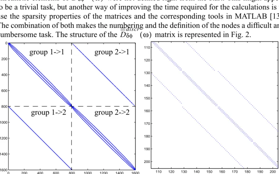
to be a trivial task, but another way of improving the time required for the calculations is to use the sparsity properties of the matrices and the corresponding tools in MATLAB [13]. The combination of both makes the numbering and the definition of the nodes a difficult and
cumbersome task. The structure of the matrix is represented in Fig. 2.
Obviously, because of the coupling between one node and its neighbours, the main diagonal of the matrix is surrounded by four other “diagonals”, as can be seen on the right-hand side of Fig. 2. These secondary “diagonals” are distorted simply because the core is not square (the unrealistic nodes are not taken into account).
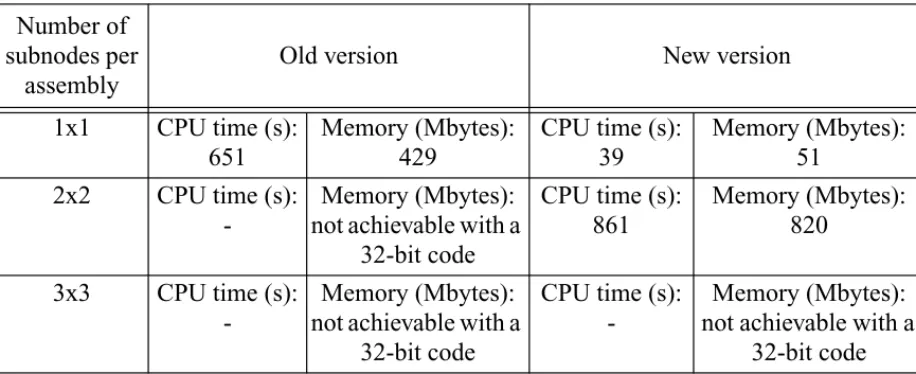
In Table III, the CPUtime and memory required for the calculation of the transfer functions for both the previous noise simulator and its new version are compared. As can be seen, it takes now only a few minutes to estimate the transfer function of a typical BWR core with 4 subnodes per assembly. Such a number of subnodes was not even achievable with the previous version. This is mainly due to the fact that the memory needed by the new simulator is significantly reduced compared to the previous one. As can be noticed also, for
Dδφdiscr( )ω Dδφdiscr( )ω Dδφdiscr( )ω Dδφdiscr( )ω 0 200 400 600 800 1000 1200 1400 1600 0 200 400 600 800 1000 1200 1400 1600 nz = 9220 110 120 130 140 150 160 170 180 190 200 110 120 130 140 150 160 170 180 190 200 nz = 9220
Fig. 2. Sparsity of the matrix (full matrix on the left-hand-side, and a closer look at the
upper left corner on the right-hand-side)
group 1->1
group 2->2 group 2->1
a BWR core like Forsmark 1 (676 fuel assemblies + 124 reflector nodes), four subnodes per assembly already correspond to the maximum number of subnodes that the new noise simulator can handle.
Another new feature of the noise simulator is that every core layout, i.e. BWR and PWR cores with different sizes can now be handled. All the user needs to do is to define a core map specifying where the fuel assemblies and the reflector nodes are located. The user also has to provide the corresponding static data (material constants and fluxes defined in maps matching the core map, and the point-kinetic parameters of the core).
1.3 Benchmarking of the simulator
Even if the cross-sections need to be adjusted before using the noise simulator, the modifications of these are almost negligible in the fuel nodes. As pointed out previously, only the fuel nodes directly neighbouring the reflector nodes are appreciably modified. Therefore locating a noise source in the middle of the core and assuming that the core is homogeneous for the estimation of an analytical solution should provide a relatively good reference solution for the numerical scheme far away from the reflector nodes.
Analytical solution in case of a central noise source
It is assumed in the following that the noise source for the analytical solution is a point source located at the core centre. Three different cases have been considered: a noise source defined in terms of the fluctuation of the fast absorption cross-section, one of the thermal absorption cross-section, and finally one of the removal cross-section. This can be formulated by writing Eq. (5) as follows:
(26)
with the following three possibilities for the noise source:
, (27)
Table III. Comparison between the old and new versions of the noise simulator
Number of subnodes per
assembly
Old version New version
1x1 CPU time (s): 651 Memory (Mbytes): 429 CPU time (s): 39 Memory (Mbytes): 51 2x2 CPU time (s): -Memory (Mbytes): not achievable with a
32-bit code CPU time (s): 861 Memory (Mbytes): 820 3x3 CPU time (s): -Memory (Mbytes): not achievable with a
32-bit code
CPU time (s):
-Memory (Mbytes): not achievable with a
32-bit code D r( )∇2+φ(r,ω) ( ) δφ1(r,ω) δφ2(r,ω) S1(r,ω) S2(r,ω) = S1(r,ω) S2(r,ω) γ ω( ) δ( )φr 1 0, ( )r 0 × =
or
, (28)
or
. (29)
Here is the noise source strength. This coefficient allows also taking into account the fact that the noise source is homogeneously distributed over one or several nodes in the numerical solution (the nodes representing the core centre), and therefore is not a point-source.
Due to the symmetry of the system, the flux noise is simply given by:
(30) (31)
where and are the two eigenvalues of the following matrix:
(32)
and the coupling coefficient and are given as follows:
(33)
(34)
The coefficients A, B, C, and D are solutions of the system:
S1(r,ω) S2(r,ω) γ ω( ) 0 δ( )φr 2 0, ( )r × = S1(r,ω) S2(r,ω) γ ω( ) δ( )φr 1 0, ( )r δ – ( )φr 1 0, ( )r × = γ ω( ) δφ1(r,ω) = A×K0( )λr +B×I0( )λr +C×Y0( )µr +D×J0( )µr δφ2(r,ω) A×cλ×K0( )λr +B×cλ×I0( )λr +C×cµ×Y0( )µr +D×cµ×J0( )µr = λ2 – µ2 Σ1( )ω ⁄D1 – νΣf 2, ( )ω ⁄D1 Σrem 0, ⁄D2 –Σa 2, ( )ω ⁄D2 cλ cµ cλ Σrem 0, Σa 2, ( )ω –D2λ2 ---= cµ Σrem 0, Σa 2, ( )ω +D2µ2 ---=
(35)
where R is the core radius (fuel + reflector zones).
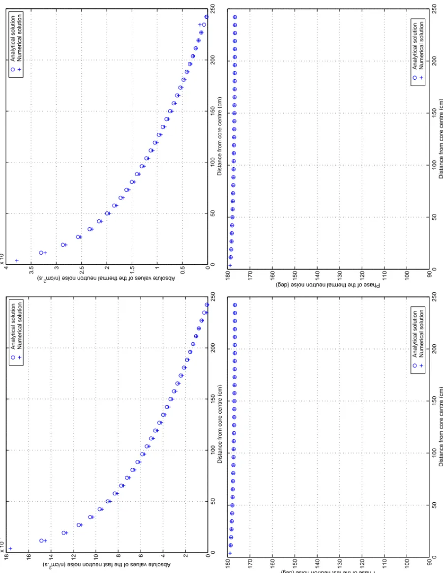
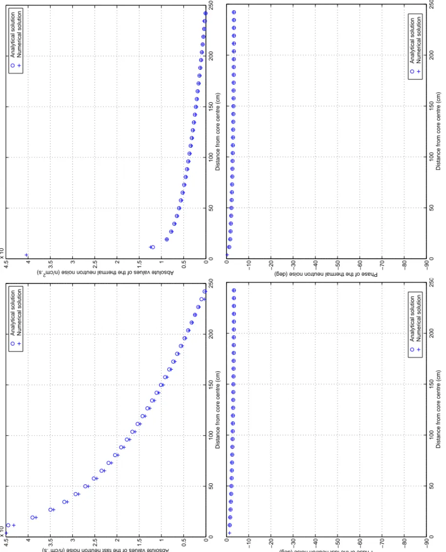
Comparison between the numerical and analytical solutions
The following figures (see Figs. 3-5) depict the amplitude of the flux noise and its phase for both the analytical solution and the numerical one. Since the noise simulator calculates a spatially-averaged flux noise over each node, the analytical solution was also averaged over each node, so that both solutions could be directly compared. The first point of the numerical solution (from the core centre) represents the flux noise in the node where the noise source is located. The analytical solution gives obviously a different solution in this node, and therefore the first point of the analytical solution was systematically disregarded.
It can be noticed that the agreement between the analytical and the numerical solutions is very good. As expected, the discrepancy is somewhat larger at the core boundary than at the core centre, due to two main reasons. The first one is simply the presence of the reflector in the numerical simulation, whereas the analytical one does not take any reflector into account. The second effect lies with the fact that close to the reflector nodes, the cross-sections have been adjusted in the noise simulator, so that the system remains critical despite the use of the finite difference scheme. Therefore, while in the analytical case the reactor is homogeneous, the core becomes more and more heterogeneous close to the core boundary in the numerical case. Since the flux noise vanishes at the core boundary, the difference between the analytical and numerical solutions is hardly noticeable for the amplitude of the noise. Even if the discrepancy regarding the phase of the flux noise slightly increases away from the core centre, the accuracy still remains very good, as can be seen on the different Figures.
Consequently, the noise simulator seems to reproduce the expected solution rather well. Despite the apparent high level of accuracy, the fact that the core is homogeneous (or more exactly almost homogeneous) has to be strongly emphasized. The finite difference scheme is a very effective (and easy to implement) discretization scheme as long as the discretised system does not present a strong level of heterogeneity. A realistic core is of course far from being homogeneous. Even if core homogeneity is still an acceptable approximation for PWRs, BWRs are highly heterogeneous systems due to the presence of
K0(λR) I0(λR) Y0(µR) J0(µR) cλ×K0(λR) cλ×I0(λR) cµ×Y0(µR) cµ×J0(µR) 1 – 0 –[µr×Y1( )µr ]r→0 0 cλ – 0 –cµ×[µr×Y1( )µr ]r→0 0 A B C D × 0 0 1 2πD1 ---
∫
S1(r,ω)dr 1 2πD2 ---∫
S2(r,ω)dr =the control rods (in a PWR, the reactivity adjustment is mainly carried out by the boron concentration). Therefore, the accuracy may deteriorate appreciably when a realistic core is modelled. One way of coping with this could be to increase the number of nodes in the numerical simulation. Nevertheless, a commercial BWR like Forsmark 1 has already 800 nodes in the radial direction (676 fuel assemblies + 124 reflector nodes). As pointed out previously, the corresponding matrix representing the transfer function is of a 1600x1600 size. Dividing each node into 4 sub-nodes is still possible, but already appears to be the
0 50 100 150 200 250 0 2 4 6 8 10 12 14 16 18 x 10 15
Distance from core centre (cm)
Absolute values of the fast neutron noise (n/cm
2
.s)
Analytical solution Numerical solution
0 50 100 150 200 250 90 100 110 120 130 140 150 160 170 180
Distance from core centre (cm)
Phase of the fast neutron noise (deg)
Analytical solution Numerical solution
0 50 100 150 200 250 0 0.5 1 1.5 2 2.5 3 3.5 4 x 10 15
Distance from core centre (cm)
Absolute values of the thermal neutron noise (n/cm
2
.s)
Analytical solution Numerical solution
0 50 100 150 200 250 90 100 110 120 130 140 150 160 170 180
Distance from core centre (cm)
Phase of the thermal neutron noise (deg)
Analytical solution Numerical solution
Fig. 3. Comparison between the analytical and numerical solutions, for the case of a fast
maximum number of nodes that a 32-bit code could permit. Consequently, an acceptable level of accuracy could only be achieved if a more efficient discretization scheme than the finite difference one is used. Nodal methods or finite elements are planned to be considered in the near future at our Department.
0 50 100 150 200 250 0 0.5 1 1.5 2 2.5 3 3.5 4 4.5 5 x 10 15
Distance from core centre (cm)
Absolute values of the fast neutron noise (n/cm
2
.s)
Analytical solution Numerical solution
0 50 100 150 200 250 90 100 110 120 130 140 150 160 170 180
Distance from core centre (cm)
Phase of the fast neutron noise (deg)
Analytical solution Numerical solution
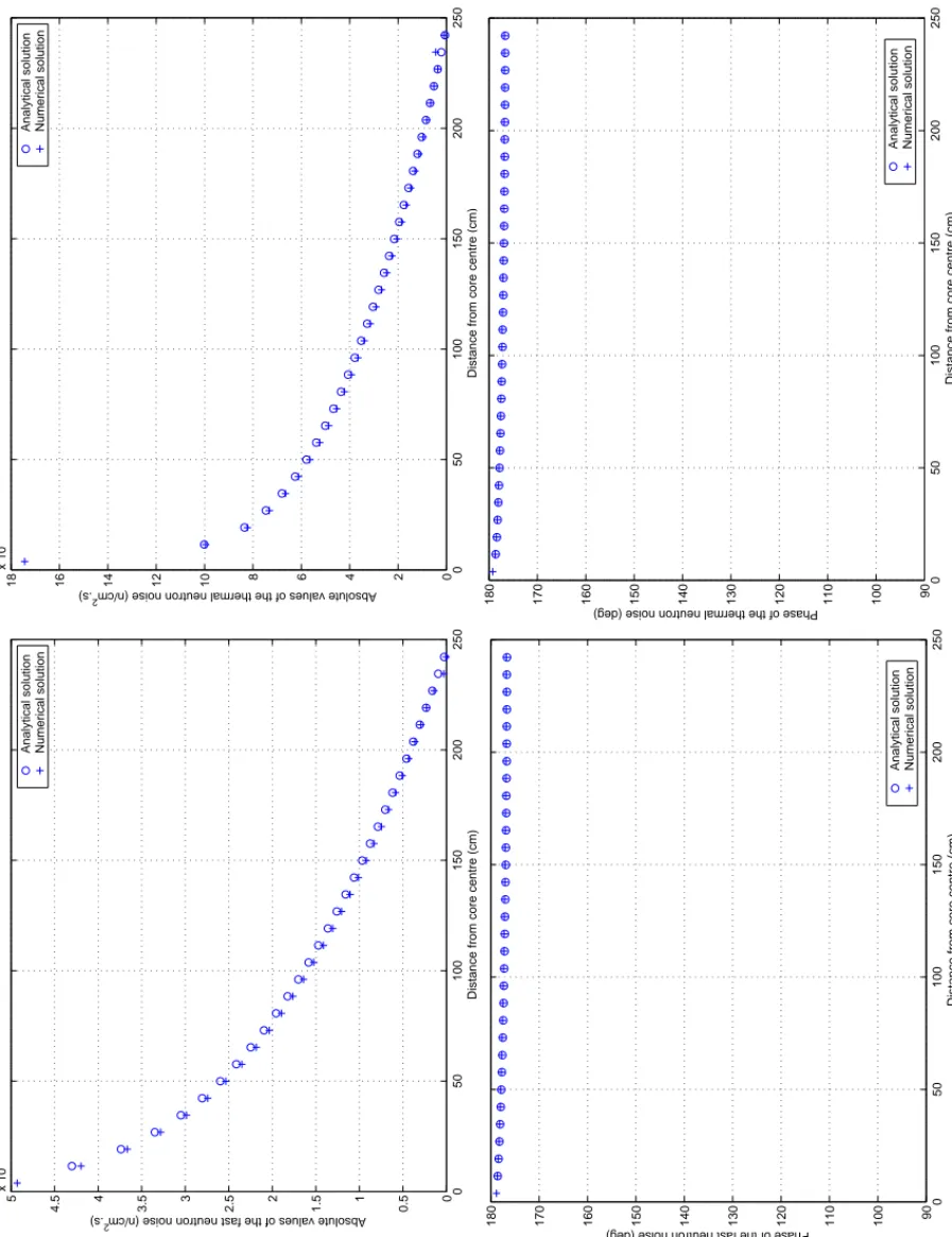
0 50 100 150 200 250 0 2 4 6 8 10 12 14 16 18 x 10 14
Distance from core centre (cm)
Absolute values of the thermal neutron noise (n/cm
2
.s)
Analytical solution Numerical solution
0 50 100 150 200 250 90 100 110 120 130 140 150 160 170 180
Distance from core centre (cm)
Phase of the thermal neutron noise (deg)
Analytical solution Numerical solution
Fig. 4. Comparison between the analytical and numerical solutions, for the case of a
1.4 Conclusions
In this Section, a 2-D 2-group neutron noise simulator, relying on the diffusion approximation, was presented. The spatial discretization scheme used is the finite difference scheme. Such a simulator was already briefly presented in stage 6, but much effort has been spent on improving the calculational efficiency since then. The noise simulator calculates the transfer function between any possible location of a noise source in
0 50 100 150 200 250 0 0.5 1 1.5 2 2.5 3 3.5 4 4.5 x 10 15
Distance from core centre (cm)
Absolute values of the fast neutron noise (n/cm
2
.s)
Analytical solution Numerical solution
0 50 100 150 200 250 −90 −80 −70 −60 −50 −40 −30 −20 −10 0
Distance from core centre (cm)
Phase of the fast neutron noise (deg)
Analytical solution Numerical solution
0 50 100 150 200 250 0 0.5 1 1.5 2 2.5 3 3.5 4 4.5 x 10 15
Distance from core centre (cm)
Absolute values of the thermal neutron noise (n/cm
2
.s)
Analytical solution Numerical solution
0 50 100 150 200 250 − 90 − 80 − 70 − 60 − 50 − 40 − 30 − 20 − 10 0
Distance from core centre (cm)
Phase of the thermal neutron noise (deg)
Analytical solution Numerical solution
Fig. 5. Comparison between the analytical and numerical solutions, for the case of a
the core and the neutron noise. Due to the large size of the matrix representing the transfer function, the calculational speed is for instance quite crucial in a diagnostic task such as the localisation algorithm reported on in the next Section. The CPUtime required to perform the calculation of a typical BWR core with 2x2 sub-nodes per assembly is now reasonable, which means that scanning a frequency range in order to estimate the frequency-dependent transfer function of the reactor seems to be realistic. Even if a fully coupled neutronic/ thermal-hydraulic 3-D noise simulator is still interesting and will be developed at a later stage, this entirely neutronic 2-D calculator allows estimating and investigating many qualitative aspects of the neutron noise in a reactor core. Some of them have already some practical applications, such as the localisation of a noise source from the detector readings (see next Section).
Even if the benchmarking of this simulator for homogeneous cores showed that the agreement between the numerical and analytical solutions was excellent for both the amplitude and the phase of the flux noise, it is believed that the accuracy could deteriorate when strongly heterogeneous cores like BWR ones are considered. This is mainly due to the fact that a finite difference scheme was used for the spatial discretization. Therefore, it appears to be appropriate to study the possibility of using a more sophisticated scheme, such as finite elements or nodal methods, for the development of a coupled neutronic/ thermal-hydraulic noise simulator. Finite elements will be given special attention since a multiphysics code, named FEMLAB, is now available at our Department.
Section 2
Application of the neutron noise simulator to anomaly localisation 2.1 Introduction
In the preceding case, the flux noise was calculated assuming that the noise source was known (both its strength and its location). Even if being able to estimate the flux noise in a reactor is undoubtedly interesting, determining the location of an unknown noise source from the neutron detector readings is even more challenging. Such an inverting capability could be directly used for diagnostic purposes. In the following, an algorithm allowing to locate the position of a noise source (but not its strength) is presented. Several test cases are also presented, so that the validity of the algorithm can be assessed. Finally, the localisation procedure is used in a practical case, namely the Forsmark 1 local instability event.
2.2 Localisation algorithm
The localisation algorithm is the one developed previously by Karlsson and Pázsit [14], [15]. Therefore, only the basic principles of this procedure are recalled in the following. More details can be found in the original papers.
If one assumes that there is only one noise source located in the node (I0, J0), the flux noise can be calculated from Eq. (21). This can be written in a condensed form as follows:
(36)
is in fact the discretised two-group Green’s function of the system,
which is evaluated by the noise simulator. Conceptually, is a 2x2
matrix and the multiplication in Eq. (36) is a matrix multiplication. Since neutron detectors are most often sensitive to the thermal flux, one can write also:
(37)
or more simply:
(38)
where is the second row of the matrix and
correspondingly the multiplication in Eqs. (37) and (38) is a scalar product.
Estimating the ratio between the flux noise measured at two different locations A and B allows eliminating the noise source strength:
δφ1 I J, , ( )ω δφ2 I J, , ( )ω G I( 0,J0→I J, ;ω) S1 I 0 J0 , , ( )ω S2 I 0 J0 , , ( )ω × = G I( 0,J0→I J, ;ω) G I( 0,J0→I J, ;ω) δφ2 I J, , ( )ω G2(I0,J0→I J, ;ω) S1 I 0 J0 , , ( )ω S2 I 0 J0 , , ( )ω × = δφ2 I J, , ( )ω = G2(I0,J0→I J, ;ω)×SI0,J0( )ω G2(I0,J0→I J, ;ω) G I( 0,J0→I J, ;ω)
(39)
The left-hand-side of Eq. (39) can be obtained from measurements. The right-hand-side contains the unknown of the problem, namely the location of the noise source. The transfer or Green’s functions can be calculated to any combination of their argument, but the source position is not known. It is given by the values for which Eq. (39) is fulfilled. The localisation algorithm will thus calculate the right-hand-side of Eq. (39) for all possible locations of a single noise source within the core and will retain the one giving the ratio of the detector signals, i.e. the left-hand-side of Eq. (39).
In reality the equality will not be complete due to background noise and other disturbing effects, thus some procedure utilising redundancy is used for a best estimate. If one has access to several detectors, the following quantity can be evaluated for each detector combination (A, B):
(40)
so that the minimum of the following function should correspond to the location of the noise source (I0, J0):
(41)
Since it is common practice to use the Auto- and Cross-Power Spectral Densities (APSDs and CPSDs respectively) of the measured signals instead of their Fourier transform, Eqs. (40)-(41) have to be written as follows:
(42)
and
(43)
Despite the apparent high number of possible detector combinations, the number of detectors quadruplets that need to be taken into account can be significantly reduced if the redundant combinations are discarded. For the sake of brevity, these simplifications are not presented here. We refer to the original paper instead [15].
δφ2 I A JA , , ( )ω δφ2 I B JB , , ( )ω --- G2(I0,J0→IA,JA;ω) G2(I0,J0→IB,JB;ω) ---= I0,J0 ( ) ∆A B, (I J, ) δφ2 I, ,A JA( )ω δφ2 I B JB , , ( )ω --- G2(I J, →IA,JA;ω) G2(I J, →IB,JB;ω) ---– = ∆(I J, ) ∆2A B, (I J, ) A B
∑
, = ∆A B C D, , , (I J, ) CPSD A B( , ,ω) CPSD C D( , ,ω) --- G2(I J, →IA,JA;ω) G2 ∗ I J I B,JB;ω → , ( ) × G2(I J, →IC,JC;ω)×G2∗(I J, →ID,JD;ω) ---– = ∆(I J, ) ∆2A B C D, , , (I J, ) A B C D, , ,∑
=2.3 Sensitivity of the algorithm
The localisation algorithm described previously can be easily tested since the noise simulator allows generating the flux noise for a given noise source. More precisely, one will assume a given location of a noise source within the core, and calculate the corresponding flux noise. The flux noise will then be used as detector signal input to the localisation algorithm. This procedure should return the (known) location of the noise source, if the localisation procedure is correct. The sensitivity of the localisation algorithm to different parameters can therefore be assessed. These parameters are the number of detector signals used, the position of the noise source, the possibility of having several noise sources, the contamination of the detector signal by external noise, and finally the transfer function used for the localisation.
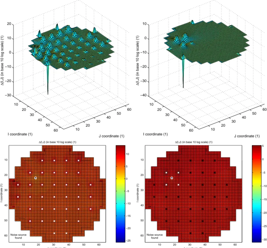
In the following, the results will be presented in two types of Figures, one depicting the function in a 3-D plot, and another one depicting also the function but in a 2-D plot (core map). In this latter case, the detectors are also positioned via crosses (‘X’). The white ones indicate the detectors used in the localisation, whereas the black ones the detectors which were not used. The noise source is marked by a white asterisk (‘*’), and the result of the localisation algorithm is denoted by a white circle (’O’). The core layout and the location of the detectors correspond to the Forsmark 1 BWR. Nevertheless, the cross-sections used in these test cases are representative of a two-region system (fuel + reflector regions), assumed to be homogeneous before the necessary adjustment of the cross-sections for criticality. More details regarding these cross-sections sets can be found in Section 2.4 “Cross-sections”.
The first Figure (Fig. 6) represents the effect of using a reduced number of detectors. The peaks in the function correspond to the detector locations. At these spots, the accuracy is better than away from the detectors. Therefore, since the noise source is not
located at any of the detector positions, a local maximum of the function is
expected. As pointed out previously, although eliminating the redundant detectors combinations allows reducing significantly the calculation time, taking all the detectors into account still requires too much CPUeffort. Furthermore, in most cases only a few number of detector signals are actually available from measurement campaigns. Therefore, the localisation algorithm was tested in two cases: first assuming that all the detectors were available, second by using only the four detectors surrounding the noise source. As can be seen in Fig. 6, the noise source is correctly located when using a reduced set of detectors. Even if using as many detectors as possible would seem to be the most logical choice, in the following test cases only the detectors neighbouring the noise source are used. This does not affect the success of the localisation algorithm negatively.
The right-hand-side of Fig. 6, together with Fig. 7, allows also noticing that the precision of the localisation algorithm is perfectly insensitive to the location of the noise source. A noise source located close to the core boundary is as successfully detected as a central one.
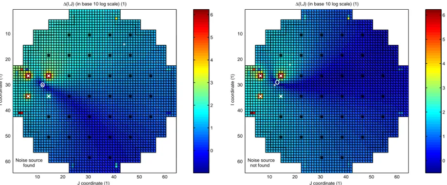
Although the localisation algorithm has been designed for locating one single noise source, it is not unlikely that more than one noise source is present in the core when actual measured signals are used. The localisation algorithm, on the other hand, is based on the assumption that there is only one noise source present. The solution, as suggested in the previous papers ([14], [15]) is that, each noise source is located from the signals of detectors that surround the source in question. This strategy works as long as the different noise sources are sufficiently separated. This assumption was tested in the simulations. As can be
∆(I J, ) ∆(I J, )
∆(I J, )
seen on Fig. 8, choosing a set of detectors positioned close to one of the noise sources allows detecting successfully the corresponding one, as long as the two noise sources are not too close.
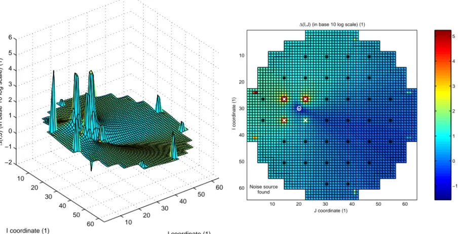
The algorithm needs also to be tested when extraneous random noise is added to the detector signals before performing the noise source localisation. As can be seen in Fig. 9, the noise source is still correctly located even with as much as 10% of extraneous noise. One could notice nevertheless that the dip in the function is less accentuated with noise than without noise (see for instance Fig. 6). The main reason that could explain why the noise source is still correctly located with a relatively high level of background noise is that in the present work, in contrast to all previous work, the noise source was assumed to be given as a perturbation of the removal cross-section. As can be seen on Figs. 3-5, the thermal flux noise decreases much more rapidly away from the source for a removal cross-section noise source than for a fast or thermal absorption cross-cross-section noise source. Therefore, using the transfer function between the removal cross-section noise and the thermal flux noise in the localisation algorithm is expected to provide a more pronounced
10 20 30 40 50 60 10 20 30 40 50 60 −30 −20 −10 0 10 20 J coordinate (1) I coordinate (1) ∆
(I,J) (in base 10 log scale) (1)
10 20 30 40 50 60 10 20 30 40 50 60 −40 −30 −20 −10 0 10 J coordinate (1) I coordinate (1) ∆
(I,J) (in base 10 log scale) (1)
−25 −20 −15 −10 −5 0 5 10 10 20 30 40 50 60 10 20 30 40 50 60
∆(I,J) (in base 10 log scale) (1)
J coordinate (1) I coordinate (1) o* Noise source found −30 −25 −20 −15 −10 −5 0 5 10 20 30 40 50 60 10 20 30 40 50 60
∆(I,J) (in base 10 log scale) (1)
J coordinate (1)
I coordinate (1)
o*
Noise source found
Fig. 6. Result of the localisation algorithm when all the detectors are used
(left-hand-side) and when only the detectors surrounding the noise source are used (right-hand-side)