Computer simulations: Orientation of Lysozyme in vacuum under the influence of an electric field

UPTEC X 11 016

Examensarbete 30 hp

Mars 2011

Computer simulations: Orientation

of Lysozyme in vacuum under the

influence of an electric field

Molecular Biotechnology Programme

Uppsala University School of Engineering

UPTEC X 11 016

Date of issue 2011-03

Alexei Abrikossov

Title (English)

Computer simulations: Orientation of Lysozyme in vacuum under

the influence of an electric field

Title (Swedish) Abstract

The possibility to orient a protein in space using an external electrical field was studied by means of molecular dynamics simulations. To model the possible conditions of an electro spray ionization (ESI) the protein Lysozyme in vacuum was considered under the influence of different field strengths. The simulations showed three distinct patterns: (1) the protein was denaturated when exposed to too strong electrical fields, above 1.5 V/nm; (2) the protein oriented without being denaturated at field strengths between 0.5 V/nm and 1.5 V/nm (3) the protein did not orient and did not denaturate if the strength of the field became to low, below 0.5 V/nm. Our simulations show that the orientation of the protein in the fields corresponding to the second pattern takes place within time intervals from about 100 ps at 1.5 V/nm to about 1 ns at 0.5 V/nm. We therefore predict, that there exists a window of field strengths, which is suitable for orientation of proteins in experimental studies without affecting their structure. The orientation of proteins potentially increases the amount of information that can be obtained from experiments such as single particle imaging. This study will therefore be beneficial for the development of such modern techniques.

Keywords

ESI, Lysozyme, Orientation, Electrical fields, Molecular dynamics, GROMACS Supervisors

David van der Spoel, Uppsala University

Carl Caleman, DESY

Scientific reviewer

Johan Elf, Uppsala University

Project name Sponsors

Language

English

ISSN 1401-2138

Supplementary bibliographical information Pages

37

Biology Education Centre Biomedical Center

Computer simulations: Orientation of Lysozyme in

vacuum under the influence of an electric field

Populärvetenskaplig sammanfattning

Alexei Abrikossov

Under en längre tid har röntgenkristallografi varit den ledande tekniken för att bestämma proteinstukturer. Det som gör det hela möjligt är kristallernas symmetri som förstärker informationen som fås under experimentet. Det som å andra sidan hämmar tekniken är själva kristalliseringen av proteiner. Vissa proteiner är nämligen väldig svåra att kristallisera, som till exempel membranproteiner. Dessa proteiner är av stor betydelse för läkemedelsutveckling och annan forskning, men är näst intill omöjliga att kristallisera. Därför forskar man nu för att få fram nya tekniker som gör att man kommer att kunna ta bilder av proteiner utan att behöva kristallisera dem först, till exempel via en teknik som heter single particle imaging. Att veta hur ens protein är orienterat under ett sådant experiment kommer att underlätta analysen av data som fås under

experimentet. Den här studien undersöker, med hjälp av simuleringar, om det är möjligt att orientera ett protein i rymden med hjälp av externa elektriska fält. Det som möjliggör en sådan orientering är det dipolmoment som varje protein har. Eftersom en dipol orienterar sig i fältets riktning kommer det att orientera hela proteinet. Frågan är dock om det går att orientera ett protein utan att samtidigt störa dess struktur. Mina resultat visar att det finns ett intervall av elektriska fältstyrkor som inducerar en orientering utan att negativt påverka proteinets veckning.

Examensarbete 30 hp

Table of contents

1. Introduction

7

2. Methods

9

2.1. Protein in the electric field 9

2.2. Molecular Dynamics

11

2.2.1. GROMACS 12

2.2.2. Leap-frog algorithm 13

2.2.3. Energy minimization 14

2.2.4. Steepest descent algorithm 14

2.2.5. Constraints 15

2.2.6. Temperature coupling 15

2.2.7. Non-bonded interactions 16

2.2.8. Periodic boundary conditions 17

2.2.9. Boxes 17

2.2.10. Electric field 18

2.3. Model Protein 19

2.4. The simulation details 20

2.4.1. Bulk simulation

20

2.4.2. Vacuum simulation

20

3. Results

22

3.1. Protein stability

25

3.2. Orientation

26

3.3. Orientation stability

32

4. Discussion and Conclusions

34

1. Introduction

For a long time x-ray crystallography has been the primary technique to determine the atomic structure of proteins. The crystal offers great advantages because the proteins that form the crystal are all aligned. The symmetry enhances the amount of information obtained from the structure. The resulting Bragg peaks that are detected with the images from the x-ray crystallography experiments, provide enough information to calculate a full atomic model of the protein if resolution is high enough. The radiation damage from the beam is also spread over a large number of molecules reducing its impact on the information. However, x-ray crystallography has one significant weakness. It is very hard to purify some proteins and force them to crystallize. For example out of the large amount of membrane proteins only a small percentage have had their structure determined in this manner.

For this reason there is a large demand for new ways of determining protein structures. One such idea was presented by Neutze et al. in 2000 [1] suggesting that single molecule coherent imaging using short x-ray pulses should be possible. There are now existing sources of hard x-rays which could be used for single molecule imaging at LCLS in Stanford and a European X-ray Free Electron Laser (XFEL) is under construction in Hamburg. Recent experiments using these sources have demonstrated that single particle imaging is feasible [2].

A method proposed to deliver single particle samples into the x-ray source is the electro-spray ionization (ESI) [3-5]. Contrary to a crystal where all proteins are ordered and aligned, an ESI injection will result in a randomly oriented sample. Since the amount of images that will be needed to reconstruct a full three dimensional model of the protein is considerable, the possibility to orient the sample prior to the snapshot being taken will certainly be beneficial during the reconstruction. Experiments on orientation of small molecules and proteins using different kinds of electric fields and aligning lasers have been going on for some time now [6], as well as calculations on how proteins behave after the ESI injection

[7-The main question of this study is to determine how the addition of an external electric field would affect the overall structure of the protein in vacuum. The concern is that the electric field needed to orient the protein will be so strong that the protein will break down well before any measurements can be made. With this in mind there is a reason to ask the question if there is damage done to the overall structure of the protein. And if so, how fast is that damage being inflicted? If the damage occurs after taking the image it will not inflict any interference with the data that is being collected. This study investigates whether there is an interval of electric fields that can provide the necessary torque for the protein to orient without any significant damage to the protein.

To test if such an interval of electric fields exists, a study was performed using molecular dynamics (MD) simulations. The advantage of using MD to simulate the behaviour of the protein under these ESI conditions is the possibility to easily change the input of the simulation, as well as obtaining a detailed visual display of what happens during a very short period of time, something an experiment can have problems to achieve.

The second question of the study is: if the protein does orient itself in the electric field, how fast would this happen? Would the orientation be fast enough to be considered practical to implement it in an experiment?

The effect of the strength of the field of the electric field has also been studied in this work, to understand how the field strength affects the structural changes and the orientation. Will different strengths affect the orientation time and the time it takes to damage the structure?

2. Methods

2.1 Protein in the electric field

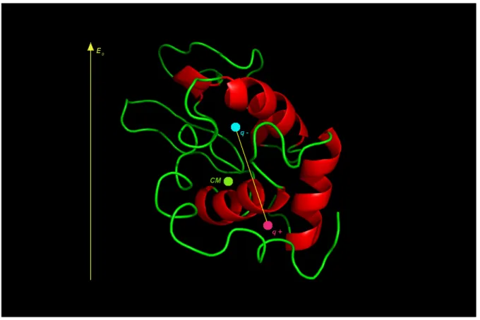
The main idea behind this study is to use the internal dipole of a protein in an electric field to orient it in space (Figure 1). The force on each of the charges in the dipole from the electric field E₀ will result in a torque that will rotate the protein.

Figure 1: A schematic representation of our model. The protein Lysozyme is used in this study. Green circle is the centre of mass (CM). The blue circle is the negative effective charge of the dipole and the magenta circle is the positive effective charge of the dipole. The yellow arrow represents the direction of the electric field E0.

The electric dipole of a protein can be described as:

p=

∑

i =1 N

q_ir_i (1)

where p is the dipole, qi is the charge of each atom, ri is the directional vector of each

atom. When a dipole is placed in an electric field _E

0 the force on the charges will be:



F_i=q_iE

0 (2)

This shows that the total force that is affecting the protein is equal to zero when

∑



=p× E₀ (3)

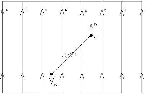
To visualise what we are dealing with one can consider a simple dipole (Figure 2) between two charges:

p=q d (4)

where d is the directional vector between the charges.

Put in an electric field (as illustrated in Figure 2) such dipole would become an ideal harmonic pendulum. By doing so it will forever oscillate without ever reaching any specific orientation. Our system is more complex (Figure 1). The protein is not rigid, thus giving it internal friction to induce a damped oscillation leading to its particular orientation in the electric field. The friction will lead to heating, which could induce unfolding.

Figure 2: Illustrating the behaviour of an ideal simple dipole in an electric field. The force F on the charges q will give rise to a torque. This will move the charges to orient the dipole in the field. Θ is the angle between the electric field and the distance vector d.

2.2 Molecular Dynamics

The basic idea of a MD simulation is as follows [9]: knowing initial coordinates of a molecular system, to compute its time evolution using classical equations of motion solved with small time steps. The information that has to be known about the system besides the positions of all the atoms ( r ) and their velocities ( v ), which can be randomly generated using Maxwellian distribution, is the potential interaction :

Thus the force acting on particle i:



F_i=− ∂V

∂ r_i , V  r1, ... , rN (5)

can be determined by calculating the sum of all the different forces from atoms j that act on the atom i:

 F_i=

∑

jFij (6)

where F_ij are forces between non-bonded atom pairs as well as the forces that arise because of bonded interactions, restraining and/or external forces. Besides calculating the force on any given atom one can also compute the potential and kinetic energies as well as the pressure tensor. The main part of the simulation is to determine how all the atoms in a system move. To do this one has to solve Newtons equations of motion for all the atoms N.

m_i∂

2_r i

∂t ²= Fi i=1,... , N (7)

Using Newton's equation of motion implies that the motion of the atoms will be described using classical mechanics. This should not pose any difficulty since this kind of description is perfectly fine for most cases with normal temperature.

2.2.1 GROMACS

To be able to perform a successful simulation on a protein there is a need to implement more than just the above mentioned ideas behind the MD. One needs a platform which incorporates numerical algorithms and takes into account such effects as temperature coupling, pressure coupling and conservation of constraints. The electric field that was used in this study must also be accounted for.

That is why several MD calculation packages have been developed over the years. The one that was used to conduct the present study is called GROMACS [10] which is an abbreviation for “GROninen MAchine for Chemical Simulations”. GROMACS was first developed at the university of Groninen in the Netherlands and the core development of GROMACS right now is done by:

• David van der Spoel at Department of Cell and Molecular Biology, Computational and Systems Biology, Uppsala University, Sweden.

• Erik Lindahl at the Center for Biomembrane Research, Department of Biochemistry & Biophysics, Stockholm University, Sweden

• Berk Hess at the Center for Biomembrane Research Department of Biochemistry & Biophysics, Stockholm University, Sweden

GROMACS is a free software package and is available under the GNU General Public License. The source code as well as a selected set of binary packages is available on the GROMACS website www.gromacs.org. The main purpose of GROMACS is to perform molecular dynamics (as described in section 2.2 and 2.2.2) and energy minimization (section 2.2.3). In the description of the methodology below we will follow Ref [11].

2.2.2 Leap-frog algorithm

The propagation is done numerically using the Leap-frog algorithm [12]. It is called so because of the way one upgrades values of the positions and velocities. By taking positions

r at time t and velocities v at time t−t

2 the algorithm updates both the positions

and velocities using the forces _{F t . The later should be calculated for positions at time t.}

This gives us the following relations, which are based on a Taylor expansion neglecting third and higher order of terms:

v tt 2 =v t− t 2   F t  m t (8) r tt=rt vtt 2  t (9)

Because of the way the time steps are used the calculations of r and v can be visualised as jumping over each other. Thus the algorithm has got its name Leap-frog.

2.2.3 Energy minimization

The potential function that describes the state of a macromolecule has a complex landscape with lots of peaks and valleys. These valleys are local minima points with one deepest point that is called the global minimum. The potential energy in this point is lower than that in other parts of the landscape. Energy minimization is the standard practice to use prior to a MD run. It gives us several possible starting structures for MD simulations. Since there are no algorithms ensuring that any given structure is in the global minimum, a local minima is what one should deal with.

2.2.4 Steepest descent algorithm

GROMACS implements several algorithms to perform the energy minimization. The one that was used during this study is the steepest descent algorithm. Although it is not a very efficient algorithm, the methods robustness and ease of implementation make it a popular tool to use.

The method is numerical. First, a vector r is defined as vector of all 3N coordinates and an initial displacement h0 is given (e.g. 0.01 nm). Then the forces F and the potential energy are calculated.

The new positions can now be calculated by:  rn1= rn  F_n max

∣

∣

Here hn is the maximum displacement, Fn is the force i.e. negative gradient of the

potential V. The notation max 

∣

_∣

force components. The forces are then again computed with the new positions. If

V_n1V_n the new positions are accepted and h_n1=1.2 h_n . On the other hand if

V_n1≥V_n the new positions are rejected and h_n=0.2 h_n . The algorithm will run for the amount of iterations that is specified by the user or until the energy converges to a minimum.

2.2.5 Constraints

During the simulation it happens that the bond lengths change due to forces. To make sure that the bond lengths correspond to the optimal ones, there are algorithms that make sure that they stay within certain bonds. The algorithm used during the study is called LINCS [13]. It is a two step algorithm that restores bond lengths after an unconstrained update. It is a fast method but can only be applied to bond constraints and some isolated angle constraints.

2.2.6 Temperature coupling

Because of several reasons such as drift during equilibration, calculation errors due to force truncation and integration errors, as well as possible heating due to external or frictional forces, there maybe a need to control the temperature of the system so that this parameter does not become unphysical and does not give unphysical effects on the results and the model. The coupling for this study was a type of weak coupling named after Berendsen [14].

The scheme of the coupling of temperature is as follows:

dT dt =

T0−T

 (11)

Thus the temperature deviation from T₀ is slowly corrected and the deviation of the temperature decreases exponentially with a time constant  , which it is defined as:

=2CvT Ndfk

(12)

Here k is Boltzmann’s constant, τT is the temperature coupling time constant, Cv is the total heat capacity of the system and Ndf is the total number of degrees of freedom. This thermostat will suppress the kinetic energy fluctuations resulting in an improper canonical ensemble.

2.2.7 Non-bonded interactions

There are many non-bonded interactions that arise in macromolecular systems, such as the Lennard-Jones interaction and the Coulomb interaction. The Lennard-Jones potential between a pair of atoms can be written as:

V_LJr_ij=Cij

12

r_ij12 −

C_ij6

r_ij6 (14)

Here Cij12 and Cij6 depend on the type of atoms that are involved in the interaction.

The r_ij is the distance between the two atoms. Coulomb potential can be written as:

V_cr_ij=f qiqj rrij

where: f =_{4 }1

0 (16)

Here ₀ is the permittivity in vacuum, _r is the dielectric constant of the media (= 1 in our case), qi and qj are the charges and rij is the distance between the charges.

The calculations that are based on these non-bonded interactions are dependent on lists of neighbouring atoms. Thus to prevent unnecessary calculations between atoms that are too far apart cut-offs are used. One can decide to have calculations done within a certain range of the atom.

2.2.8 Periodic boundary conditions

Periodic boundary conditions are used to minimize the effect of edges of a finite system. The atoms of the simulated system are placed in a box. This box is then surrounded by translated copies. This way there would not be any edges or boundaries present. When an atom leaves the box it will re-appear on the other side from a neighbouring box. The artifacts caused by the edges of the system are thereby suppressed by periodicity. This can be desired especially when calculating on crystals although it can be problematic when one is dealing with non-periodic substances as liquids.

2.2.9 Boxes

There are a lot of different types of boxes that exist to realize the periodic boundary conditions and a cubic box might not always be the best way to go when dealing with a certain problem. For example, a rhombic dodecahedron is more suitable when simulating a spherical or a flexible molecule in a solvent, because the volume that such a box will occupy is only 71 % of a cubic box thus saving the CPU time by 29 %. In our study though we used a cubic box in the bulk simulation (default box) and no box was used in the vacuum

2.2.10 Electric field

The current version of the GROMACS package has an implementation that allows one to apply an electric field to the system [15]. The field is implemented to be a laser pulse and is described by the following expression:

Et =E₀e

−t −t0 2

2 2 

cost−t₀ (17)

Here Et  is the field at time t and t0 is the starting time (=0 in our case) , E0 is the

maximum amplitude of the field,  is the length of the pulse and:

=2  c  (18)

In equation 18 c is the speed of light in vacuum and  is the wavelength of the laser. In this study to simulate a constant electric field (DC field), both  and  were chosen in such a way that made both the cos and ex function to be close to one. This gives us the approximation:

2.3 Model Protein

The protein chosen to be the test protein in this study was chicken hen egg-white Lysozyme (1AKI ) [16]. It is well characterized and not too large for MD simulations. Indeed the

protein is 129 amino acids long and according to the protein data bank (PDB) has a weight of 14331.20 Daltons. Lysozyme is a globular protein that consists mainly of helices and loops. The crystal structure that was downloaded from the Protein Data Bank had a resolution of 1.5 Å [16]. There were two other reasons for choosing this protein to be the test object of the study. The first was that Lysozyme does not change its charge in vacuum as was shown experimentally [7]. The second was that the protein had undergone studies that simulated its stability in vacuum [7-8]. These studies showed that although there were changes in the structure during vacuum simulations the overall structure was mostly unchanged and the protein was stable. Those studies would therefore give us a good reference point when we evaluate our results.

2.4 Simulation details

2.4.1 Bulk simulation

The bulk simulation was performed following the description by A. Patriksson et al [7]. The pdb structure was transformed to file formats that should be used during the GROMACS simulations. The force field that was used during the simulation was OPLS-AA [17-19] and the water model was TIP4P [20]. The protein was solvated in a cubic box and subjected to a 10 ns simulation using periodic boundary conditions. This configuration was first energy minimized using the steepest descent algorithm until the system reached the energy minimum within the machine precision. After that a short 10 ps simulation was carried out during which the protein was subjected to position restraints. The final 10 ns simulation was performed using Berendsen weak coupling [14] to keep the temperature at 300 K and the pressure at 1 bar. The constants for temperature and pressure coupling was 0.1 ps and 20 ps, respectively. To limit the van der Waals interaction we used a twin range cut-off of 0.9/1.4 nm. PME algorithm [21,22] was used for Coulomb interactions with a 0.9 nm boundary. The bond lengths were constraint using the LINCS algorithm [13]. The time step during the simulation was 2 fs. The results were saved every 5000 iterations . The simulation was run using GROMACS 4.0.5 [10]. The bulk simulation was performed to allow the protein to equilibrate under physiological conditions.

2.4.2 Vacuum simulation

The vacuum simulation began by extracting the protein structure from the bulk simulation and removing the waters from the file. Then some of the residues had to be charged accordingly [15]:

R21, R45, R68, R73, K96, R114, K116, and R128

The unsolvated protein was put in a big cubic box with 15 Å to each edge. The protein was subjected to an energy minimization and a 10 ps run with position restraints. After this a simulation for 100 ps using 1 fs as a time step was carried out. In the latter case to simulate protein in vacuum there were no periodic boundary conditions as well as no pressure or temperature couplings. The cut-offs for van der Waals and Coulomb interactions were turned off so all interactions were computed. From this 100 ps run we extracted positions of all the particles and their velocities each 10 ps resulting in 10 different starting configurations and velocity distributions. Each of these structures were then run at different electric fields strengths:

E₀=3, 2.5, 2, 1.5, 1.25, 1, 0.75, 0.6, 0.5, 0.4, 0.3, 0.2, 0.1, 0.05 V /nm

An additional run was made without the presence of an electric field for control. The electric field was applied along the x-axis. Since the protein is charged and thus had a net force acting on it, the centre of mass translation was removed during the simulation. The simulations lasted for approximately 7 ns. The positions were saved every 0.25 ps while forces and velocities every 1 ps.

3 Results

The resulting trajectories showed three distinct patterns of behaviour depending on the strength of the field.

1) Orienting and deformation. At high field strengths above 1.5 V/nm the protein showed clear signs of denaturation with the total unfolding at 3 V/nm (Figure 4) and clearly visible deformation of the protein structure at 2.5 and 2 V/nm.

2) Orienting. The intermediate field strengths 1.5 to 0.5 V/nm (Figure 5) oriented after a certain time. There were no clear structural changes to the protein although the higher fields 1.5 to 1 V/nm showed instinctive indications to a possible structure loss if the simulation had lasted longer.

3) No orientation. The lower field strengths 0.4 V/nm and lower did not induce any orientation on the protein.

Figures 4 and 5 demonstrate the first and the second types of patterns above. Figure 4 shows a typical example of the protein structure obtained at high field (pattern 1) where the protein is denaturated. In Figure 5 one sees a successful orientation of the protein in the field with the intermediate strength (pattern 2).

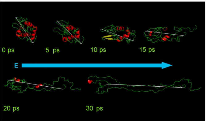
Figure 4: The unfolding of Lysozyme at a field strength of 3 V/nm. The images were taken 0, 5, 10, 15, 20 and 30 ps into the simulation. The electric field is oriented along the x-axis (blue arrow). The main chain is green and the helices are red. The white line is a schematic representation of the proteins dipole.

Let us consider Figure 4. At 0 ps we show the protein at the moment when the field is turned on. At 5 ps we see that the protein has started to orient in the electric field. The structure is still mostly intact. At 10 ps the protein is oriented in the electric field, but the deformation has already begun and most of the structure has already been lost. At 15 ps the protein is being pulled apart by the electric field, thought the protein still appears to be globular. At 20 ps the protein has been torn apart further separating the “head” from the “tail”. At 30 ps the protein is now basically 2 strands of amino acids. During this entire time frame the protein remained oriented in the electrical field.

Figure 5: Orientation of Lysozyme in the electric field of the strength 0.6 V/nm. The main chain is shown in green, alfa-helices are red and the beta-structure is yellow. The white line is the schematic representation of the dipole. The field is in the x-axis (blue arrow). The frames are taken at 0, 40, 140, 300, 500, 600, 700 and 1000 ps. The orientation is reached between 500 and 600 ps.

A different behaviour is seen in Figure 5. Here again the 0 ps gives the image of the protein the instant the field is switched on. (It is the same structure as the 0 ps in Figure 4.) The images at 40 to 300 ps show how the protein orients in the field. The images for 500 to 1000 ps show that despite some tumbling the orientation in x-axis remains the same and the protein structure is largely preserved.

3.1 Protein stability

We analyse the stability of the protein during the simulation by calculating the root mean square displasment (RMSD) of the C-alpha carbons. The RMSD is defined by the following expression [11]: RMSDt1, t2=[ 1 M

∑

∣

∣

Here r is the coordinate of atom i at at time t, mi is its mass, N is the total amount of

atoms, M=

_∑

i=1 N

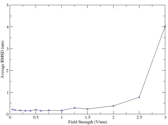
m_i , t2 represents the time for the reference structure ( t2 = 0), while t1 is the time at the particular time-step. RMSD was then averaged over the entire simulation time to get an average RMSD for a specific field-strength. By calculating the RMSD we get a good indication on how much the structure changes during the run. A big RMSD indicates a big structural change. Thus as small as possible RMSD is wanted. To figure out the effect of the electric field on the structure the RMSD is a good analysis tool to use. As previous study showed [7] the increase in RMSD is expected to a certain degree even in stable proteins, since the protein is not surrounded by water. Thus the RMSD of 0.3 nm is considered normal. Anything above 0.3 nm can be considered as an indication of the effect of the electric field on the structure. Figure 6 shows the average RMSD for all of the different field strengths that were used. As can be seen, the simulation at 3 V/nm field strength completely unfolded the protein resulting in a RMSD of 4 nm. Approximately 1 nm RMSD for 2.5 V/nm field strength also indicates a structural break. The rest of the field strengths do not seem to heavily disrupt the structure during the time of the run. However there are indications of structural changes at fields above 1.5 V/nm.

Figure 6: Average RMSD from one starting structure at different field strengths. One can clearly see that at high electrical fields the protein looses most of its structure.

3.2 Orientation

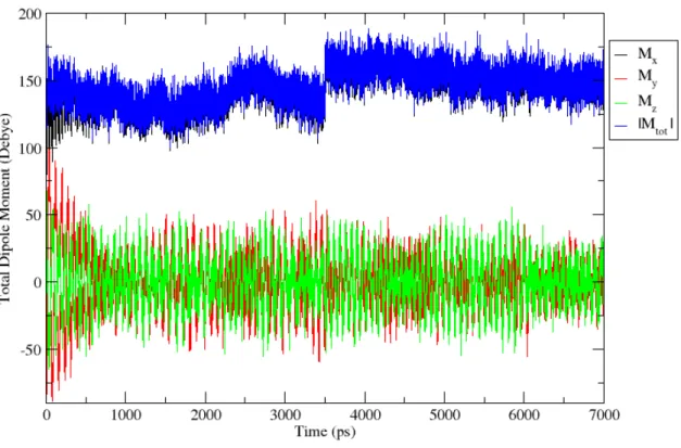
Since the main idea of this study is to see if the internal dipole moment of a protein could be used to orient it in an electric field it is crucial to study the behaviour of the dipole during the simulation. The theory states that the dipole will orient in the field due to the force on the corresponding negative and positive charges and the resulting torque. To be fully oriented the entire dipole of the protein should be along the electric field. Figure 7 shows that the total dipole moment of the system will eventually converge to its x component .

Figure 7: Example of time evolution of the dipole moment of the system at a field strength of 0.6 V/nm. The blue line indicates the total dipole of the system. Black line is the x-axis component of the dipole. Red line is the y component and the green line is the z component. Since in our case the electric field is along the x-axis the protein is considered oriented when the systems x component of the dipole equals the total dipole moment.

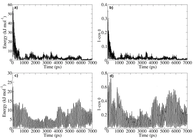
Since the electric field is in our simulations in the direction of the x-axis the convergence indicates the orientation. A better way of visualising this result is to take the cos θ between the x component and the total dipole. When the cos θ converges towards one the system converges towards orientation in the electric field. But since cos θ provides data that is relatively hard to work with, it is simpler to work with 1-cos θ (Figure 8b). This combination will make the data converge to zero instead of one and is easier to work with during further

Figure 8: a) Centre of mass rotational energy at a field strength of 0.6 V/nm. b) Example of

convergence of 1- cos θ at a field strength 0.6 V/nm. c) The rotational energy of the protein

at a field strength of 0.2 V/nm. d) Example of non-convergence of 1-cos θ at a field strength of 0.2 V/nm. Comparing the data from two different data sets confirms the orientation of Lysozyme at field-strength 0.6 V/nm a and b. Panels c and d indicate that there were no orientation of the protein at the given field strength of 0.2 V/nm. The 0.2 V/nm is oscillating around the x-axis.

Another way to check for orientation is to look at the rotational energy of the centre of mass (Figure 8a and 8c). The rotational energy will indicate if the protein has stopped its rotation, thus achieving orientation in our conditions. This data can also be used to complement the results obtained from the study of the dipole moment. Comparing panels a to b and panels c to d in Figure 8 it can be seen that the graphs appear very similar, showing us that there is more than just one data set suggesting if the orientation has taken place.

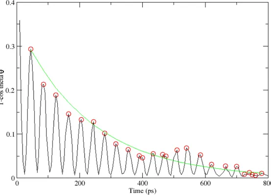
To clearer determine the way how the protein comes into orientation, one can study the part of the graph that shows orientation exclusively. By doing so one can derive useful data about the physical aspects of the orientation. As can be seen in Figure 9. The motion of the protein can approximately be described as a physical pendulum using the following differential equation [23]:

∂2 ∂t2 2 

∂

∂t 0² =0 (20)

Here  represents the position of the pendulum. The velocity of the pendulum will then

be ∂

∂t and the acceleration ∂2

∂t2 , =

b

2I where I is the moment of inertia of the protein and b is the damping factor, ₀ is angular frequency of the pendulum.

Equation (20) can be rewritten as:

I∂ 2  ∂t2 b ∂ ∂t qEd =0 (21)

Here q is the charge of the dipole, E is the electric field strength and d is distance from the charge to the point of rotation.

Figure 9: The first 800 ps of the 1-cos θ convergence at the field strength of 0.6 V/nm. This graph clearly shows that the orientation of Lysozyme follows the path of a damped pendulum. If we isolate the maximum values of the oscillation (red circles) and do an exponential regression on them (green line) we can determine the damping factor for the oscillation.

Since the oscillation is sinusoidal, it has a period T0 and an angular frequency 0 , which

are given by:

T0=2_ 0

=2



If the damping factor b is small the solution to equation (20) will be:

t= A e−t

cost (23)

and since =b

2I the damping factor can be recovered by doing an exponential regression on the maximums of the graph in Figure 10 [23]. From the γ one can get an idea of how fast the protein will orient in a given field.

Table 1: Average damping of the system at field strengths 0.4 V/nm to 0.75 V/nm

E₀ Average γ

0.4 V/nm 0.0014

0.5 V/nm 0.0034

0.6 V/nm 0.0034

0.75 V/nm 0.0031

Table 1 shows the results of exponential regression that was performed. One can see substantial increase of the damping factor γ with the field increase from 0.4 V/nm to 0.5 V/nm.

Unfortunately the higher field strengths converged so fast that a good regression did not seem possible. This indicates that the damping increases substantially between the field strengths of 0.75 V/nm and 1 V/nm.

By studying the peaks in Figure 9 one can also determine the oscillation period T0,which in

Figure 10: Time during which the protein stays oriented in the simulation. Each point represents 100ps during which the protein is considered oriented. Blue circles are the data obtained from the analysis of the dipole. Red squares are received from the analysis of the rotational energy data by mean square displacement.

3.3 Orientation stability

Since the protein was determined to be able to orient it is interesting to examine how fast it orients and if it stayed oriented during the entire simulation run or if the orientation was unstable and the protein lost its orientation later during the run. To do so we have plotted the orientation as a function of time for all the simulated electric fields in Figure 10. The time it takes the protein to orient varies between approximately 100 ps for field strengths of 1 V/nm and above to approximately 1000 ps at 0.5 V/nm. The loss of orientation by the protein can

As can be seen in Figure 10, the higher the electric field is, the less chance the protein has to lose its orientation. On the other hand as can be seen from the RMSD results (Figure 6) high electric fields tend to deform the protein.

Figure 11 demonstrates the relative time the protein stayed oriented during the run at a certain field strength. This graph can be used to determine the estimated time the protein will be oriented during the usage of other field strengths, as compared to the ones used in this study. With the average RMSD displayed in the same graph protein stability is also taken into account. From Figure 11 we therefore predict that there exists a window of field strengths, which are suitable for orientation of proteins in experimental studies without affecting their structure significantly.

Figure 11: Relative time the protein is determined to be oriented during the run. Red is data from the study of the dipole. Blue is the data from the study of the rotational energy. The difference between the two curves is within statistical uncertainty. The blue triangles represent the average RMSD. One can compare the amount of time in orientation with structure stability. The green area is the interval of fields that induce orientation without

4. Discussion and Conclusions

In this study we investigated if it is possible to orient a protein in the electric field. Using molecular dynamics we performed simulations that showed a possibility to use external electrical fields as a source to induce torque. Prior to the study there was concern that the proteins structure would break down upon the fields application. Our results indicate that this is the case only if the used fields are too strong. However if the strength of the field is too low there will not be enough force to orient the protein in the field. Therefore the fields strength must be carefully chosen in the interval that induces orientation without causing damage to the structure.

The RMSD results of the study are in accordance with results of previous studies that were on protein stability in vacuum, thus indicating that the results of protein stability are quite accurate and reproducible.

Once oriented, the protein is relatively stable in that orientation. Unfortunately there is no information to compare these results to yet. Thus the reliability of the orientation results needs further studies to be confirmed.

When the orientation of the protein is confirmed to be stable by further studies, one may attempt to control the orientation process and turn the protein in any way that one wishes. To get there a lot of questions must be answered. For example is our model applicable on other proteins. In this study the protein Lysozyme was used as a model, but how good does this model represent proteins in general? Lysozyme is relatively small and good knowledge about how it behaves during MD simulations is present, thus making it a good model protein to work with. The variety of proteins is very large and a lot of the proteins form some sort of complexes: with other proteins, with nucleic acids or with lipids. How would such a complex fare in under the conditions of this study? Another aspect that will be interesting to examine is the possibility to use several fields in different directions, since in our case we only examined a one dimensional orientation leaving the protein free to rotate around the

Another question is how to actually orient the protein, the fields that were used to orient the protein in this study are only theoretical, a practical implementation of these fields can prove very difficult due to their strength (1 V/nm = 1 GV/m which is very high). A step in the right direction would be to test how an alternating current (AC) field (laser) would affect the orientation ability of the protein. The main question in such a case would be what magnitude of the wave length should be used. In our study we concluded that the orientation time can range from tens to thousands of picoseconds (Figure 11) and the wavelengths that orient the protein in an AC field should be possible to achieve. A more practical question would then also be as follows: assuming that the theoretical part is complete what would be the correct way to implement this knowledge practically?

In summary, by means of molecular dynamics simulations we show that Lysozyme tends to loose its structure when the strength of the electrical field rises above 1.5 V/nm and does not react to the field if the strength is bellow 0.5 V/nm. At the same time, we predict that at field strengths between 0.5 V/nm and 1.5 V/nm orientation should take place. The possibility to orient a protein with external fields without its destruction is an important conclusion of this work, which should be of interest for the researchers who are currently working on perfecting the techniques that are meant to bring us toward single particle imaging.

5. References

[1] Neutze, R., Wouts, R., van der Spoel, D., Weckert, E., Hajdu, J. (2000) Potential for

biomolecular imaging with femtosecond X-ray pulses, Nature 406, 752-757.

[2] Chapman, H., N., Fromme, P., Barty, A., et. al. (2011) Femtosecond X-ray protein

nanocrystallography, Nature 470, 73-77.

[3] Yamashita, M., and Fenn, J. B. (1984) Electrospray ion source. Another variation on the

free-jet theme, J Phys. Chem. 88, 4451- 4459.

[4] Yamashita, M., and Fenn, J. B. (1984) Negative ion production with the electrospray ion

source, J Phys. Chem. 88, 4671- 4675.

[5] Fenn, J.B., Mann, M., Meng, C. K., Wong, S. F., and Whitehouse, C. M. (1989)

Electrospray ionization for mass spectrometry of large biomolecules, Science 246, 64-71.

[6] Lee, K.F., Villeneuve, D.M., Corkum, P.B., Stolow, A., and Underwood J. G. (2006)

Field-Free Three-Dimensional Alignment of Polyatomic Molecules, Phys. Rev. Letters

[7] Patriksson, A., Marklund, E., and van der Spoel, D. (2007) Protein conformations under

electrospray conditions, Biochemistry, 46, 933-945.

[8] Marklund, E., Larsson D.S.D., van der Spoel D., Patrikson A. and Caleman C. (2009)

Structural stability of electrosprayed proteins: temperature and hydration effects, Phys.

Chem Chem. Phys., 11, 8069-8078.

[9] van Gunsteren, W. F., Berendsen, H. J. C. (1990) Computer simulation of molecular

dynamics: Methodology, applications, and perspectives in chemistry, Angew. Chem. Int. Ed.

Engl., 29, 992–1023.

[10] van der Spoel, D., Lindahl, E., Hess, B., Groenhof, G., Mark, A. E., Berendsen, H. J. C. (2005) GROMACS: Fast, Flexible and Free, J. Comp. Chem. 26, 1701–1718.

[11] van der Spoel, D., Lindahl, E., Hess, B., van Buuren, A. R., Apol, E., Meulenhoff, P. J., Tieleman, D. P., Sijbers, A. L. T. M., Feenstra, K. A., van Drunen R.,

Berendsen, H. J. C., (2005) Gromacs User Manual version 4.0, www.gromacs.org

[12] van Gunsteren, W. F., Berendsen, H. J. C. (1988) A leap-frog algorithm for stochastic

dynamics, Mol. Sim. 1, 173–185.

[13] Hess, B., Bekker, H., Berendsen, H. J. C., and Fraaije, J. G. E. M. (1997) LINCS: A

linear constraint solver for molecular simulations, J. Comput. Chem. 18, 1463-1472.

[15] Caleman C. and van der Spoel D. (2008) Picosecond, Melting of Ice by an Infrared

Laser Pulse: A simulation study, Angew. Chem. Int. Ed. , 47, 1417-1420.

[16] Artymiuk, P. J., Blake, C. C. F., Rice, D. W., and Wilson, K. S. (1982) The structures of

the monoclinic and orthorombic forms of hen egg-white lysozyme at 6 Ångstroms resolution,

Acta Crystallogr.,Sect.B, 38, 778.

[17] Jorgensen, W. L., and Tirado-Rives, J. (1988) The OPLS potential functions for

proteins. Energy minimizations for crystals of cyclic peptides and crambin, J. Am. Chem.

Soc. 110, 1657-1666.

[18] Jorgensen, W. L. (1998) in Encyclopedia of Computational Chemistry, Vol. 3, pp 1986-1989, Wiley, New York.

[19] Kaminski, G. A., Friesner, R. A., Tirado-Rives, J., and Jorgensen, W. L. (2001)

Evaluation and reparametrization of the OPLS-AA force field for proteins via comparison with accurate quantum chemical calculations on peptides, J. Phys. Chem. B 105, 6474-

6487.

[20] Jorgensen, W. L., Chandrasekhar, J., Madura, J. D., Impey, R. W., and Klein, M. L. (1983) Comparison of simple potential functions for simulating liquid water, J. Chem. Phys. 79, 926- 935.

[21] Darden, T., York, D., and Pedersen, L. (1993) Particle mesh Ewald: An N-log(N)

method for Ewald sums in large systems, J. Chem. Phys. 98, 10089-10092.

[22] Essmann, U., Perera, L., Berkowitz, M. L., Darden, T., Lee, H., and Pedersen, L. G. (1995) A smooth particle mesh ewald method, J. Chem. Phys. 103, 8577-8592.

[23] González M. I. and Bol A. (2006) Controlled damping of a physical pendulum: