HaGPipe
Programming the graphics pipeline in Haskell
Tobias Bexelius (tobias bexelius@hotmail.com)
M¨
alardalen University
Abstract
In this paper I present the domain specific language HaGPipe for graphics pro-gramming in Haskell. HaGPipe has a clean, purely functional and strongly typed interface and targets the whole graphics pipeline including the programmable shaders of the GPU. It can be extended for use with various backends and this paper provides two different ones. The first one generates vertex and fragment shaders in Cg for the GPU, and the second one generates vertex shader code for the SPUs on PlayStation 3. I will demonstrate HaGPipe’s many capabilities of producing optimized code, including an extensible rewrite rule framework, automatic packing of vertex data, common sub expression elimination and both automatic basic block level vectorization and loop vectorization through the use of structures of arrays.
Contents
1 Introduction 2
2 Haskell 101 5
3 The pipeline 11
4 Programs as abstract syntax trees 13 5 General numerics 18 6 The expression types 21 7 Rewrite rules 23 8 Border control 27
9 Post pass 31
10 Wrapping it all up 35 10.1 Cg vertex and fragment shader backend . . . 36 10.2 SPU vertex shader backend . . . 36 11 Results & conclusions 39 12 Discussion & future work 42 13 Related work 44 14 Acknowledgments 45
Chapter 1
Introduction
3D-graphics is a computationally heavy duty; in the current state of the art a graphics pipeline model shown in figure 1.1 is used in which a stream of 3D objects represented as triangles are transformed and rasterized into pixel fragments, which gets lit and merged into a 2D image1 shown on the screen.
Figure 1.1: The graphics pipeline.
Vertex buffer Input assembler
Vertex shader Vertices
Rasterizer
Vertices with positions in canonical view space Constants
Fragment shader Fragments
Output merger
Color and depth values Constants and textures
Front buffer
Since no global state is updated, this process is highly parallelizable, and this is why most personal computers have a special purpose GPU (Graphics Processing Unit) dedicated for this task. For the last decade, the vertex and fragment shader stages has become programmable,2 providing a highly
cus-tomizable graphics pipeline.
All triangles sent into the pipeline are represented by three vertices where
1This is called the front buffer.
2Newer hardware also have a programmable geometry shader stage between the vertex
each vertex have a position in 3D and usually some additional attributes, such as normal vectors, texture coordinates and color values. The vertex shader is a function that (in parallel) transforms each incoming vertex with attribute data into a new vertex with 3D-positions in canonical view space (i.e. where x, y, z ∈ [−1, 1] will be visible in the resulting frame) and possibly some altered attribute data.
The rasterizer uses the transformed positions of each triangles vertices to generate pixel fragments for all pixels covered by the triangle in the resulting image. The vertices attribute data outputted from the vertex shader will also get interpolated for all pixel fragments over the triangle.
The fragment shader is then executed (in parallel) for each generated pixel fragment and computes each fragments final color and depth value. The depth values can be used by the output merger to filter out fragments hidden by other triangles’ fragments.
Two major APIs (Application Programming Interfaces) have evolved for the task of managing and programming GPUs: OpenGl and DirectX. For the programmable shader stages, both APIs have incorporated their own shader languages; OpenGl has GLSL and DirectX has HLSL. The graphics card man-ufacturer NVidia has also created Cg, a shading language supported by both OpenGl and DirectX. Such shading languages are examples of domain specific languages, as opposed to general purpose languages such as C++, Java and Haskell.
When programming the graphics pipeline using one of the APIs above, the common workflow consists of first writing vertex and fragment shaders in one of the supported shader languages, and then writing a “host” program (usually in C or C++) that loads and uses those shaders as well as sets up the other non-programmable stages of the pipeline. In this paper I suggest another approach, and present HaGPipe3, a DSL (Domain Specific Language) where we program
the graphics pipeline as a whole. The difference between HaGPipe and the shader languages described earlier is that HaGPipe is embedded in Haskell, a functional language for general purpose programming with several interesting properties. A listing of Haskell’s many features are provided in the next chapter for those of you that haven’t had the opportunity to try this amazing language out yet.
The goal of HaGPipe for the purpose of this paper is to generate the vertex and fragment shader programs. I will provide backends for generating Cg-code and for generating C++-code for the SPUs (Synergetic Processing Units, the coprocessors) of PlayStation 3. HaGPipe is implemented as a Haskell library that may be imported by a programmer in order to write shaders in Haskell. The programmer won’t even need to define what backend should be used. Instead, a third part may use the shader written with HaGPipe to generate code for several different backends. The actual code generation will occur when we run the Haskell program in which the backend’s generator function is applied to the HaGPipe shader. The produced code may then be compiled by a third party shader compiler and used in a host program. If the host program is written in Haskell, there is also the opportunity to embed the HaGPipe code directly into the host program, in order to generate and compile the shaders at the same time
3“HaGPipe” is an abbreviation of Haskell graphics pipeline, but also reminiscent to
as the host program that will use them is being compiled. I’ll briefly discuss this and other possible additions to HaGPipe in chapter 12. Instead, I’ll let the main focus of this paper be the process of transforming HaGPipe into optimized shader code.
Chapter 2
Haskell 101
Haskell [16] [10] [9] has shown to be an ideal host language for EDSLs (Em-bedded Domain Specific Languages1) [6] [8] [18], and there is a wide range of different EDSLs implemented in Haskell already, even for graphics program-ming.2 Haskell is a deep language, and takes some time to fully understand. The purpose of this chapter is not to give a complete tutorial of the language, but rather to demonstrate the benefits of using it in the HaGPipe project, and to explain its rather uncommon syntax.
Haskell is a functional language, and as such the use of functions is empha-sized. The syntax for applying functions in Haskell is very concise; actually a separating whitespace is used for function application. Instead of writing f(x,y) as is common in other languages, we simply write f x y. Another syn-tactic feature of Haskell is that almost every non-alphanumeric character string may be used as an operator, e.g. ++, >>= or :>>. All operators in Haskell are binary, except for the unary minus (-) operator. Any function may be used as an operator by enclosing it in ampersands, e.g. x ‘f‘ y is equal to f x y. Dually, any operator may be used as a standard prefix function by enclosing it in parantheses, e.g. (+) x y is equal to x + y.
Haskell has many interesting, and in some cases unique, features:
Purity. The result of a function in Haskell is only defined on its input; given the same input twice, a function will always return the same output. This makes expressions in Haskell referentially transparent, i.e. it never mat-ters if two identical expressions share the same memory or not. As a consequence, the sub expression f a in the expression g (f a) (f a) only needs to be evaluated once, and the result can safely be reused for both parameters of the function g.
Immutable data. All data in Haskell is persistent, i.e. never changes once created. All functions operating on data in Haskell will always return a new version of the data, leaving the old version intact. Without mutable data, Haskell has no for- or while-loops, and recursion is the only way to create loops.
1Another common abbreviation is DSEL, Domain Specific Embedded Languages. 2See chapter 13.
Laziness. Since pure functions are only defined on their input, and since all data is persistent, it doesn’t matter when an expression is evaluated. This makes it possible to delay the evaluation of a value until it’s needed, a strategy called lazy evaluation. This will optimize away unneeded com-putations, as well as make it possible to define infinite data structures without running out of memory.
Higher order functions. In Haskell, functions are first class values and may be passed as arguments to or returned as results from other functions. In fact, a function taking two parameters is actually a function taking one parameter, returning a function taking another parameter, that in turn returns the resulting value. You could partially evaluate a function in Haskell by supplying only some of the left-most arguments, a technique called “currying”3. With operators both operands may be curried, e.g.
(4/) is a function taking one parameter that returns 4 divided by that parameter, and (/4) is a function also taking one parameter but returns the parameter divided by 4.
Closures. Creating functions in Haskell is easy: you could for instance use a function to create another function, curry a function with one or more parameters, or use a lambda expression. With lambda expressions, an anonymous function can be defined at the same time it’s used, which for instance is useful when you need to define a function to be used as argument to another function. A lambda expression can be used whereever a normal function name can be used. An example of a lambda expression is (\ a b -> abs a + abs b) which is a function taking two arguments, a and b, that returns the sum of their absolute values. Common for all these ways of creating functions is that they may contain variables from the surrounding scope, which requires those values to be retained in memory for as long as the created function may be used. The retaining of a value in a function is called a closure, and is a feature not only found in Haskell, but most languages with automatic memory management, such as C# and Java.
Strong polymorphic types with type inference. All data types in Haskell are statically determined at compile time, and types can also be param-eterized, like templates in C++ or generics in Java and .Net. Haskell in-corporates type inference, which means that the type of an expression or variable can be deduced from its context by the compiler so the program-mer won’t have to explicitly write it. This is not the same as dynamic typing where expression has no type at all; in Haskell the type checker will generate an error if no unambiguous type could be deduced from the context.
Data types in Haskell are declared with this syntax:
data BinaryTree a = Branch (BinaryTree a) (BinaryTree a) | Leaf a In this example, BinaryTree a is a parameterized type with two data con-structors, Branch and Leaf, which holds different kind of member data. All
type names and their data constructors must start with an upper case charac-ter, and a data constructor can have the same name as its type. Functions on the other hand must start with a lower case character. BinaryTree is called a type constructor, since it’s excpecting a type parameter a.
A Branch has two BinaryTree’s (with the same parameter type a) and the Leaf has a single value of type a. A BinaryTree value has the form of one of these constructors, i.e. either it’s a branch with two sub trees, or it’s a leaf with a value. A type could have any number of constructors.4 A data constructor could be seen as a function only that it won’t get evaluated into some other value. A binary operator could be used as a type or data constructor if it starts with a colon (:), such as :> as we’ll see later on in this paper. The colon operator itself is a data constructor in the Haskell list type that concatenates a list element with a trailing sub list.
Some built in data types that are commonly used in Haskell are lists and tuples. Lists can contain a variable number of elements of one type and tuples can contain a specific number of elements of different types. A list type is written by enclosing the element type inside square brackets (e.g. [Int]) and a tuple is written as a comma separated sequence of types enclosed by normal parantheses (e.g. (String,Int,Int)).
Deconstructing a data type is done using pattern matching, as in the follow-ing example:
count x (Branch y z) = count x y + count x z count x (Leaf y) | x == y = 1
| otherwise = 0
In this example, the function count is a function taking two parameters that counts the number of occurrences of a specific element (supplied in the first parameter) in a BinaryTree (provided as second argument). It has two definitions where the first matches the constructor Branch for the second pa-rameter, and binds the variable x for the first parameter and the variables y and z for the Branch’s data members (the sub trees). The second definition matches the constructor Leaf on the second parameter instead, and also has two guarded paths. The first path is taken if the variables x and y are equal, otherwise the second path is taken. otherwise is actually just a constant with the value True. Function patterns are tried in order from the top down, and the definition of the first matching pattern with a passed guard expression will be the result of the function application. Since Haskell is strongly typed, all definitions of a function must have matching types. In this case for example, the second parameter must always be a BinaryTree a.
The last example also highlights another syntactic feature of Haskell, layout rules. In Haskell, the indentation actually has a syntactic meaning and is used instead of a lot of curly braces ({}) to group statements together, as could be seen in other languages. This is why the second guarded line was intended to match the previous one. One big advantage with the layout rule is that the programmer is forced to write well formatted code.
4In fact, a type may even have no constructors, but in this case no values can have this
type. Such a type may only be used as a type parameter in a phantom type, explained later in this chapter.
Type synonyms could be declared with the type keyword as in this example:
type BinaryStringTree = BinaryTree String
The type of a function is expressed with ->. For example, the type of the function count in our example above will be inferred to a -> BinaryTree a -> Int, i.e. a function taking a value of type a, a BinaryTree a and returns an in-teger value. Actually, this is only partly true. The actual type would be Eq a => a -> BinaryTree a -> Int, saying that a must be an instance of the type class Eq. The => keyword is used to denote a context for a type. The type variables (e.g. a in our previous example) can be restricted to belong to specific type classes by stating this on the left side of =>. Type classes are used in Haskell to share interface between different data types, and is similar to in-terfaces in Java or .Net. Type classes are actually the only way to overload a function or operator for different data types in the same scope in Haskell. The declaration of a type class looks like this:
class Eq a where
(==) :: a -> a -> Bool (/=) :: a -> a -> Bool
This class has one type variable a and two operators == and /= that all instances of this class must implement. The :: keyword is used to denote the type of a function or expression in Haskell. A type class is implemented by this syntax:
instance Eq (BinaryTree a) where
Branch x y == Branch z w = x == z && y == w Leaf x == Leaf y = x == y
_ == _ = False
x /= y = not (x == y)
In this example we also see the use of pattern wildcards (_) that is matching any expression and not bound to any variables. In an extension to standard Haskell, a type class may have more than one type variable, and could be used to express relations between types, something we’ll utilize frequently in HaGPipe. Subclasses can be defined by restricting what types that can be instances of a class by using =>, as in the following example where Ord is a subclass of the Eq class:
class Eq a => Ord a where compare :: a -> a -> Ordering (<) :: a -> a -> Bool (>=) :: a -> a -> Bool (>) :: a -> a -> Bool (<=) :: a -> a -> Bool max :: a -> a -> a min :: a -> a -> a
Given that functions in Haskell have no side effects, one might wonder how to actually perform any work in Haskell. Monads [20] are one of the more advanced features in Haskell that provides the means for effectful computing to Haskell. A monad is a “wrapper” type with two defined operations. These two operations are called return and >>= in Haskell, and is declared in a type class as:
class Monad m where return :: a -> m a
(>>=) :: m a -> (a -> m b) -> m b
This class is actually not implemented on types, but on type constructors. We can see that m in the method declarations above is always used with a parameter (a or b) and thus must be a type constructor expecting one type parameter. A monadic value is called an action, e.g. the type constructor IO implements the Monad class so the type IO String is an IO-action that results in a String. The method return creates a simple action that wraps up a value in a monad. The resulting value from an action could be used by the >>= operation to create a new action in the same monad. Writing monadic actions in Haskell is made easy thanks to the do-notation. By using the keyword do we could instead of m = a >>= (\ x -> b >>= (\ y -> c >>= (_ -> d x y))) just write m = do x <- a y <- b c d x y
Every row of a do statement is a monadic action, in our example the actions are a, b, c and d x y. The order of evaluation is implied by the order of the rows. The <- keyword is used to bind the (unwrapped) result of a monadic action to a local variable. Besides the wrapped up values, monads may also contain an internal state that is passed along by the >>= operator. For example with the Reader monad its easy to pass along an read-only environment value without the need of explicitly wire it through all functions. In the State monad, the internal state value is also writeable. With the IO monad, the internal state is the entire world, so this monad could be used to write stateful code that for instance accesses the file system or writes to the screen. The main function in a Haskell program is a value of type IO (), i.e. an IO-action returning a trivial () value (i.e. nothing). Since the constructor of the IO type is private, this main function is the only way of getting a “handle” to the outside world. The definition of the Monad class ensures that the internal state of the IO monad never may be copied or retrieved, neither can we execute IO-actions from within
a pure function.5 As an example of how the IO monad is used, consider this
simple Haskell program: main =
do
putStrLn "Enter your name:" name <- getLine
putStrLn ("Hello " ++ name)
The first row writes a prompt to the screen, the second reads input from the keyboard, and the third writes a greeting back to the screen. Thanks to the do notation, imperative programming in Haskell is as simple as that.
5Actually, with the function unsafePerformIO this could indeed be done, but as the name
Chapter 3
The pipeline
We start by defining a polymorphic data type GpuStream a, which represents a stream of as on the GPU. A stream is an abstraction of vertices, primitives, fragments, pictures etc streaming through the graphics pipeline. As mentioned before, for the sake of this paper we’ll limit ourselves to streams of vertices and fragments.
newtype GpuStream a = GpuStream a instance Functor GpuStream where
fmap f (GpuStream a) = GpuStream (f a)
The data type GpuStream is polymorphic, not only to incorporate both ver-tices and fragments, but also the different attribute combinations they may have. A “vertex” or “fragment” may be any combination of types representable in a shader, e.g. floating point values or vectors. A vertex may for instance be represented as a position vector and a normal vector. By letting GpuStream become an instance of the standard library Functor class, we can operate on the vertices or fragments running through the stream. The Functor class is defined as:
class Functor f where
fmap :: (a -> b) -> f a -> f b
fmap takes a function and in our case an GpuStream, and applies the function to all elements of the stream, resulting in a new stream. This corresponds to using a vertex or fragment shader, but in a more modular way. It is possible to fuse several operations together by applying fmap several times on different functions. We may also use the same polymorphic functions both on general purpose code as well as in shaders.
To transform a stream of vertices to a stream of fragments we use the function rasterize. The declarations of this function’s type is shown below:
rasterize ::
GpuStream (VPosition, v) ->
GpuStream (FPosition, FFace, FWinPos, f) type VPosition = V4 (Float :> Vertex) type FPosition = V4 (Float :> Fragment) type FFace = Float :> Fragment type FWinPos = V2 (Float :> Fragment)
This function takes a stream of vertex positions paired with some data and returns a stream of fragment positions, grouped with their facing coefficients, window positions and rasterized data.1 The type class ShaderRasterizable is
used to constraint the data that can be transferred over the shader boundaries. This type class will be defined as we cover the border control in chapter 8. We can also see a lot of new types such as V4, V2, :>, Vertex and Fragment in the definitions above.2 These types will also be defined in the following chapters.
To generate shader code, we use the functions vertexProgram and fragmentProgram to extract information for the different shader stages:
vertexProgram ::
(VertexIn v, FragmentOut r) =>
(GpuStream v -> GpuStream (SMaybe r Fragment)) -> Shader ()
fragmentProgram ::
(VertexIn v, FragmentOut r) =>
(GpuStream v -> GpuStream (SMaybe r Fragment)) -> Shader ()
Both of these functions take a pipeline function as argument and return a Shader (). The Shader type will be explained in detail in the next chapter. A pipeline function is a transformation of a vertex stream of some input type (i.e. an instance of the VertexIn class) to a fragment stream of some output type (i.e. an instance of the FragmentOut class). These type classes will also be defined in chapter 8.
1One might expect the rasterize function to require input on how to rasterize the vertices,
e.g. what kind of primitives are used and if multi sampling should be used. To keep things simple in this paper, we assume that these parameters are already set by the host program.
2Remember that since :> starts with a colon, it could be used as a parameterized type
Chapter 4
Programs as abstract
syntax trees
Now that we’ve defined the pipeline wide combinators, let’s focus on what we can do with those GpuStreams when we use the fmap function. As an example before we dig into the details, let’s see how a Phong [17] shader would look like in HaGPipe:
main = do
(writeFile "vertex.spu.cpp" . generateSPU . vertexProgram) pipeline (writeFile "fragment.cg" . generateCg . fragmentProgram) pipeline pipeline = fmap fragShader . rasterize . fmap vertShader
vertShader (vInPosition, vInNormal) =
(canonicalPos, (vertexNormal, vertexWorldPos)) where
model = uniform "modelmatrix" proj = uniform "projmatrix" norm = convert model
homPos = vInPosition .: V4 x y z (const 1) worldPos = model * homPos
canonicalPos = proj * worldPos vertexNormal = norm * vInNormal vertexWorldPos = convert worldPos
fragShader (fragmentViewPos, _, _, (fragmentNormal , fragmentWorldPos)) = toSMaybe (Just (fragmentColor, z fragmentViewPos))
where
a = 30
lightPos = uniform "lightpos" material = uniform "material" eyePos = uniform "eyepos"
l = normalize (lightPos - fragmentWorldPos) r = reflect (-l) n
v = normalize (eyePos - fragmentWorldPos) ambient = x material
diffuse = pure (l * n) .* y material
specular = iff (r * v > 0) (pure ((r * v) ** a) .* z material) 0 fragmentColor = saturate
(iff (l * n > 0) (ambient + diffuse + specular) ambient) What this program does (in the main action), is that it generates source code
for a vertex shader and a fragment shader and writes it to disc. The function pipeline in this program is our complete render pipeline. Note that we won’t actually “run” this pipeline with any data in this program, just turn it into two text files containing source code written in some other shader languages.
The functions vertShader and fragShader is mapped over the streams of vertices and fragments respectively, and this is where all the work gets done. The . operator is used to compose functions together just as ◦ in mathematics. In vertShader we transform the position in model space to world space with a model matrix, and then use a perspective projection matrix to get the coordinate in the canonical view space. The vertices’ normals are transformed accordingly using the model matrix. The rasterizer uses the canonical view coordinate to interpolate the world position and normal over the generated fragments. The fragShader function then use these interpolated values to calculate a Phong shaded color for each fragment. The resulting color consists of three components: ambient color, diffuse color and specular color. Ambient color is a constant component, diffuse color is computed from the angle between the normal and the incoming light, and the specular is computed from the angle between the reflected light and the viewers direction. The dot product is used to get the cosine of the angle between two vectors. We need to use some iff expressions1
to make sure that fragments that aren’t facing the light doesn’t get diffuse or specular lighting. The function pure above is used to create a vector of values from a scalar value, and .* is used for component-wise multiplication of vectors. The operator .: is called “swizzling” and is defined in the next chapter. The noraml arithmetic operators +, - and * are extended to apply to vectors and matrices as well, e.g. * between a matrix and a vector (as in worldPos above) is a matrix multiplication, while it’s defined as the dot product when used between two vectors (as in l * n above). a ** b is defined in Haskell as “a raised to the power of b”.
We now want to take the functions vertShader and fragShader and some-how turn them into shader code, but there is no way to inspect a function programmatically in Haskell. The solution is to use a special data type for the output of those functions that instead of containing a resulting value contains the expression used to compute that value. This expression can then be turned into shader code, e.g. in Cg, and saved to file. In order to get a resulting ex-pression from the functions we need to feed them a symbolic input value that acts as a placeholder for the actual input that will be given to the shaders. We need to define this expression data type and the operators we use on it in the vertex and fragment shaders. For the expression type, we use an abstract
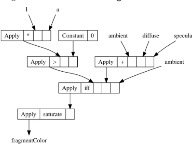
tax tree (AST). An abstract syntax tree is a data structure used in compilers that is generated by the source code parser [3]. As an example, the AST for the variable fragmentColor in the Phong shader above would look something like figure 4.1.
Figure 4.1: AST for the fragmentColor variable.
Apply * Apply > Constant 0 Apply iff Apply + Apply saturate fragmentColor ambient ambient l n diffuse specular
The AST data type is defined in HaGPipe as an algebraic data type rep-resenting a dynamically typed expression tree. The leaves are either symbols represented by the Symbol data type that represents the shader input attributes and other shader variables, or constant values represented by the OrdDynamic data type, that is a variant of the type Dynamic2that also supports comparison and equality. This is important because we need to be able to sort and compare different ASTs in many rewrite rules. The branch nodes, created with the Apply constructor, are applications of operators (represented by the type Op) to lists of operand ASTs: data AST = Symb Symbol | Constant OrdDynamic | Apply Op [AST] data Symbol =
Variable Int TypeRep | -- A common sub expression SamplerAttribute String TypeRep | -- A global sampler attribute UniformAttribute String Int | -- A global uniform attribute VertexAttribute Int | -- A custom vertex input attribute FragmentAttribute Int TypeRep | -- A custom fragment input attribute FragmentPosition | -- A fragments canonical view position
FragmentFace | -- The fragments’ triangles’ normals’ z-component FragmentWPos | -- The fragments 2D window position
FragmentColor Int | -- The resulting color of a fragment FragmentDepth Int | -- The resulting depth of a fragment
FragmentDiscard -- A boolean telling if the fragment is discarded
2This type can wrap any value that implements the Typeable class, i.e. types that supports
Some things are worth mentioning regarding the AST. Firstly, the number and order of arguments are dependent on the operator, e.g. the iff operator al-ways has three arguments where the first denotes the conditional expression, the second contains the result if it’s true and the third if it’s false. Some operators can also have a variable number of operands, e.g. the + operator in figure 4.1 has three parameters. Secondly, all sub expressions will get aggressively inlined, e.g. ambient in figure 4.1 gets instantiated two times for the different branches of the iff expression. In section 9, I will present a technique that eliminates such common sub expressions.
The creation and parsing of ASTs will be split into three phases: 1. Creation, local optimization and normalization
2. Global transformation 3. Code generation
Each of those steps is dependent on which backend we want to use, e.g. there are backends where vector operations aren’t intrinsic and must be expanded into scalar operations, and since we want to support many different backends we’ll need to create some intermediate value that the backend can consume later on. We’ll also see that it’s advantageous to perform local optimizations and normalization as the AST is being built, so here we have a problem; on one hand we want to start transforming the tree right away, but on the other hand we want to wait for the backend. An elegant solution to this problem is to use monads.
The Shader monad we’ve already seen is actually a type alias, defined as:
type Shader a = ErrorT String (StateT Declarations (Reader Capability)) a type Declarations = Map Symbol AST
type Capability = Op -> Bool
The Shader monad consists of several monad transformers wrapped up to-gether. Monad transformers [11] provide a convenient way of creating a com-posite monad by adding features to a base monad. The mtl package contains several useful monad transformers, some of which we’ll use here. Simply put, a monad transformer wraps another monad instead of just a value. For instance StateT is a monad transformer that adds an internal state to another monad, thus giving it the same features as the State monad. For our Shader monad, we choose to start with a Reader monad as base that can hold a back end-specific capability function of type Op -> Bool with which we could ask the backend which operators it supports. On top of that, we wrap a StateT monad trans-former that adds an internal state remembering symbols declared throughout the pipeline. Lastly, we would like to add the ability to abort the creation of an AST and to use alternative ways instead. The ErrorT monad transformer we use for this makes our monad an instance of the MonadPlus type class, which provides abort capabilities with the mzero constant, and the possibility to add alternative paths with the mplus method. The ErrorT could also hold an error message in case of an aborted action. Another common Haskell data type that is an instance of the MonadPlus type class is Maybe a, that has the constructors Just a and Nothing and can denote a value (of the parameter type a) or the
lack of one. Having a Maybe inside all other layers of monad transformers has unfortunately shown to result in a monad that consumes all available memory and terminates with an exception. Using an ErrorT monad transformer on the top of our monad transformer stack solves that problem and makes the code run in constant memory instead. We’ll see how to use the mplus and mzero methods when we discuss rewrite rules later in chapter 7. We will hang around inside the Shader monad for the rest of the compilation process, and it’s not until we wrap it all up in chapter 10 that we’ll find our way out of it.
Now that we have a better understanding of the Shader monad, let’s go back to the functions rasterize, vertexProgram and fragmentProgram we declared in the previous chapter. Thay all have in common that they operate on the internal state of the Shader monad. rasterize actually stores away the symbols the vertex shader produces into the Shader monad’s state. Us-ing vertexProgram will throw away everythUs-ing happenUs-ing after rasterization, and fragmentProgram everything before. These two functions both return a Shader (), i.e. a shader but no return value; the backend will get what it needs from the Shader’s internal state.
Having the AST dynamically typed greatly simplifies its usage as the dif-ferent constructors to match against are kept at a minimum. However, we do need to be able to reflect the type at some point. For applications, the operator data type Op3 has a data member of type TypeRep that represents the return
type of the operation. TypeRep is also used in the data type Symbol to alleviate the need to look it up in the definition table of the Shader monad. Some sym-bols are always of a specific type (e.g. FragmentPosition) and consequently doesn’t need a TypeRep. The data type OrdDynamic used for constants also uses a TypeRep internally to save the original type. But since the AST is dynamically typed, we don’t want to expose it to the shader programmers directly. Instead we’ll wrap it in some other expression types on which we can define strongly typed functions and operators.
Chapter 5
General numerics
For the expression types I’m about to define, it would be swell if we could overload numerical literals, as well as inherit the standard prelude operators +, -, *, /, etc, in order to make shader programming as transparent as possible. We also need all overloaded operators to be closed under expression types, i.e. any operator taking expression types as input must return an expression type as output. Haskells built in numerical classes are indeed overloadable, but they are unfortunately not general enough for our specific needs:
• All classes are subclasses of the Show class, and thus must be able to convert into a String type.
• Most of the classes are subclasses of the Eq class, and methods in this class return values of the Bool type.
• The * operator are defined as type a -> a -> a, and can neither be used for type safe matrix multiplications nor for dot products.
The first of these issues are according to myself just a result of bad design choices. The latter two on the other hand origins from the lack of multi parameter type classes (which isn’t standard Haskell). We could choose to create new operators with the same name and just hide the prelude ones, but in that case we would lose the ability to overload numerical literals. The solution to these problems is preventing the standard prelude from being imported in GHC with the {-# LANGUAGE NoImplicitPrelude #-} pragma, which will make it possible for us to define new numerical classes without these limitations and let numerical literals use our classes instead. Since our classes will be more general than the ones in the prelude, we may even let all types that are instances of the old ones become instances of the new ones. One drawback of using this approach is that shader code cannot make use of existing functions that rely on the old numerical classes.
The new numerical classes we define differ from the old ones in the following ways:
• We define a class Boolean for boolean operators such as && that we imple-ment both for the standrad Bool type as well as our own bool expression type.
• We define a class If that provides a method iff that generalizes the built in if keyword to operate on different Boolean instances. Note that using iff on a bool expression type will return the conditional expression itself. • We define a class Equal1 of two parameters to parameterize the kind of
Boolean that the equality and non-equality operators return.
• The new Ord class will also take two parameters to parameterize the kind of Boolean that is returned.
• The class OrdBase provides the methods that don’t rely on a Boolean type, like min and max.
• The class RealFloatCond provides the methods of the RealFloat class that needs to be parameterized on the type of Boolean, e.g. isInfinity. • The class Mult provides the * operator.
Every graphics API provides some vector math modules and this package is no exception. To be brief, my Vector module defines the types V1 a, V2 a, V3 a and V4 a which essentially are homogenic tuples, parameterized on the type a, of length 1, 2, 3 and 4 respectively. These types all have one data constructor each of the same name as the type. Matrix types are simply defined as type synonyms for vectors of vectors. The module also defines all vector and matrix operations as methods in type classes with some appropriate default implementations, along with vector and matrix instances for all the new numerical classes we defined above.
The * operator defined in our numeric classes is defined for (type safe) matrix-matrix, vector-matrix, matrix-vector and vector-vector multiplication. The latter is simply defined as the dot product. To keep the number of different operators at a minimum,2 we define the matrix-vector and vector-matrix
mul-tiplications as matrix-matrix multiplication on column and row vectors respec-tively. For this we use the conversion functions toCmat and toRmat to convert the input vectors to matrices, and fromRmat and fromCmat to convert the re-sults back to vectors. We see that fromRmat . toRmat and fromCmat . toCmat equals the identity function, but also that toRmat . fromCmat and toCmat . fromRmat both translates into the transpose function. These properties can be utilized by our rewrite rule framework that we’ll encounter in chapter 7.
Swizzling is an operator in shading languages that creates a new vector by selecting components from another vector. In the language Cg for example, v.wyy returns a three component vector with the first element set to the w component of vector v and the second and third one set to component y. This is a nifty feature that makes it easy for a shader programmer to create a new vector by selecting components from an old one, and this API should incorporate a similar facility too. We define the functions x, y, z and w that extracts single components from vectors. With appropriate type classes, the function x work on all vector types, y on vectors of at least two elements, and so on. Since the dot (.) that is used for swizzling in other languages already is defined as
1We still want to be able to access the old class Eq, hence we don’t use that name for our
Equal class.
2This increases the number of opportunities for rewrite rules to fire. See chapter 7 for more
function composition in Haskell, we define the operator .: as our swizzling operator instead. On its left hand is the vector to extract the elements from, and on the right is a vector of functions to use on the left hand vector. The expression v .: V3 w y y will create a V3 vector with components set to the w-, y- and y-components from the vector v. Any function may be elements of the right hand vector, so our swizzling operator could also for instance be used for homogenizing vectors with the expression a .: V4 x y z (const 1). I present the definition of .: below, just to demonstrate how compact definitions may be in Haskell when utilizing higher order types and currying (see chapter 2):
(.:) v = fmap ($ v) where the standard library define
Chapter 6
The expression types
With all these new classes in place, we can go on with defining the expression types. We need different types for different kinds of expressions, e.g. bools, ints and floats. We could define many different expression types, but a simpler solu-tion is to make a polymorphic data type that uses a phantom type [7] parameter. A type parameter that isn’t used in any of the parameterized type’s construc-tors is called a phantom type parameter. It’s used to restrict the parameterized type further.
newtype x :> c = E (Shader AST) data Fragment
data Vertex
This type is just a newtype of an AST wrapped in a Shader monad. newtype works as a data construct, with the restriction that it can only have one con-structor (in our case E) with one datum (in our case a Shader AST) but the benefit of having no memory overhead. This type has actually two phantom type parameters: one for the type being expressed, and one for the context in which the type is expressed. For the purpose of this paper, we have only two contexts: Vertex and Fragment. These symbols are simply defined as data types without constructors. The use of an infix type constructor makes it easier to understand the meaning of such types, e.g. Float :> Vertex means “a Float in a Vertex”.1 The context parameter ensures that values in a vertex shader
cannot be used in fragment shaders, and vice versa. The function rasterize de-fined in chapter 3 is the only way to convert from Vertex to Fragment, and the opposite is not allowed at all. But most importantly, with the declaration of contexts we can define functions that are only allowed in one context. E.g. texturing functions are only allowed in fragment shaders.
Now let’s stop for a moment and consider an important issue: pattern match-ing on expression types. Up to this point, the special :> data type may seem to suffice for all possible expressions. But what happens if we want to repre-sent vectors in shaders? Well, couldn’t we just, for instance, use the data type V4 Float :> Vertex? This would be rather unpractical, because we would
need to define some kind of extraction function to retrieve the elements, since the whole vector would have been wrapped into a single AST. We would like to keep the ability to use pattern matching to bind variables to the elements of the V4 constructor. The solution is to wrap only the atomic types, like Float, which in our previous example gives us the type V4 (Float :> Vertex). The difference is subtle but important. Now we have a vector of (Shader wrapped) ASTs instead of a single AST. The next question is: what happens with opera-tions that take such vectors as input? For element wise operaopera-tions like +, we can simply map that operation on to the elements, as one would do with a “normal” vector. But for operations like vecLength that returns the length of a vector, we need to be able to take the whole vector as input (and thus as a single AST). For this reason the type class :>> is defined:
class a :>> t | a->t where fromAST :: Shader AST -> a toAST :: a -> Shader AST liftedType :: a -> TypeRep
This class has methods to convert an unwrapped value (e.g. a vector) into a single AST and back again. It also contains the method liftedType to return the TypeRep of the “lifted” type (i.e. the left operator of the :> type). With this class we no longer define our operations only for the :> data type, but for all types instantiating the :>> type class. The constraint a :>> c could be read “a is expressible in context c”. This class also declares a functional dependency between its type variables with the expression a->t that means that type t is dependent on type a, i.e. the compilers type inferer can infere the second type variable if it knows the first. The instance (a :> t) :>> t is trivial (e.g. fromAST = E), but for tuples, vectors and other composite types we need to create some structure AST to be able to represent the type as a single AST. HaGPipe defines many instances of the :>> class that uses an special structure AST node2on the elements of the data type.
One big caveat with the :>> class is that the instances must be single con-structor types, since we can’t know at run time (of the Haskell program) what constructor to convert back to when fromAST is used. With this limitation, and with the fact that the type :> is not an instance of the Eq class (since the values can’t be compared at run time of the Haskell program, but only when the shader executes on the GPU), there will actually never be more than one pattern to match against, and the pattern matching facility will just be used to bind variables to the constructor’s arguments. This is however in my opinion valuable enough to justify the need for the :>> class. In chapter 8 I will present the data type SMaybe that actually has two constructors, but only one of them will be used by the fromAST function.
Chapter 7
Rewrite rules
As I stated earlier, the Op data type represents an operation in our abstract syn-tax tree. Internally, its represented by a String, a TypeRep and a RewriteRule:
data Op = Op String TypeRep RewriteRule type RewriteRule = Op -> [AST] -> Shader AST
The String denotes the operator’s opcode and is used to identify the opera-tion. The TypeRep is used to save the type of the operations returned expression. The last parameter, the rewrite rule, is a function that is used to locally simplify and normalize a sub AST. Normalization in this context is the process in which an AST is transformed into a certain “normal form” to increase the chance of it being equal to another sub AST later on. E.g. in order to get (a*b) + (b*a) to be simplified into 2*a*b, the operands of one of the multiplications needs to be reordered. The “normal form” in this case could be to order the operands in alphabetical order, yielding (a*b) + (a*b) where the plus operator now can see that it has two identical operands.
A rewrite rule is invoked by the function apply as soon as the AST node is created,1thus avoiding an additional traversal of the created AST.
apply :: Op -> [AST] -> Shader AST apply op xs = getRewriteRule op op xs
where
getRewriteRule (Op _ _ r) = r
Rules that uses functions or values with the expression’s lifted type in2must
capture that function or value in a closure at the same time as the operator is created, due to the lack of full type reflection in Haskell.3 If we did had full type
reflection, we could have had a function taking an Op and return the rewrite rule. But, instead we need to save the rewrite rule as a part of the operation, in
1Or, actually, since Haskell uses lazy evaluation, as late as when the value of the AST is
needed the first time.
2An example of such a type specific rule is constant folding.
3We can get a TypeRep from a type by using the typeOf function on an undefined value
case a node on a higher level in the AST want to create a new AST node using the same operator but different operands.
The most trivial rewrite rule is ruleEnd that just returns an Apply node with the provided operation and operands. But before returning, this rule also invokes the monadic action support to ensure that the operation is supported by the backend. Here will our Shader monad come into play:
ruleEnd :: RewriteRule ruleEnd op xs =
do
support op
return (Apply op xs)
Executing the support action will retrieve the capability function from the Reader monad, applying it on the provided operation and if it returns False result in the action throwing an exception using our ErrorT monad transformer, i.e. becoming mzero. Note that we don’t need to know the capability as the expression is being built. This is what’s so ingenious with monads; the HaGPipe expression won’t actually return an AST, but a (rather large) action that, when run by the specific backend, will return our AST. Haskell’s laziness and the way ErrorT is defined ensures that no performance penalty is paid.
But what other rules than ruleEnd can we use, and how do we declare alter-native paths in the Shader monad? Executing the support action might result in the containing action aborting with an exception, so what should happen then? For this, we use some rewrite rule combinators:
type RewriteRuleC = ([AST] -> Shader AST) -> RewriteRule (>+>) :: RewriteRuleC -> RewriteRule -> RewriteRule (>->) :: RewriteRule -> RewriteRule -> RewriteRule infixr 5 >+>
infixr 4 >->
(>+>) f g op xs = f (g op) op xs ‘mplus‘ g op xs (>->) f g op xs = f op xs ‘mplus‘ g op xs
The infixr keyword declares the operator as right associative and states it’s precedence. Besides the combinators >+> and >-> we also defined the type RewriteRuleC, a rule continuation. A continuation is a function that receives a function as argument that it will apply to its result instead of returning it. With >+> we can bind several rules together, or more precisely a rule continu-ation with a rule. Since >+> is right associative, we can bind several continua-tions together and terminate the chain with the ruleEnd rule. The rewrite rule a >+> b >+> c >+> ruleEnd will run transformation a first, giving it the op-portunity to either return some AST or pass the (possibly altered) operand list on to rule b, and so on until ruleEnd returns an Apply node with the resulting operands (unless the support action yield mzero). Every step created with >+> also creates an alternative path in the MonadPlus with the mplus combinator
where the alternative is to skip the left hand rule continuation. This means that if rule a in the example above decides to transform the expression or any of its operands into a non-supported application,4 rule a will be abandoned and the
input to rule a will be fed to rule b instead. If the same happens in rule b, rule c will fire and so on.
The definition of the >-> combinator looks very similar to the one for >+>, but its behavior is quite different. This combinator is used to declare fallback rules. First of all, both its operands are RewriteRules, secondly its precedence is lower than the one for >+>. a >+> b >-> c >+> d means “try rule a >+> b first and if no valid path is returned, run rule c >+> d”. Several fallbacks can be attached in a chain where highest priority comes first.
Now that we have all these rewrite rule combinators we can finally define some rewrite rules! The HaGPipe package defines over 30 rewrite rules that is used by the :> type’s instances of the numerical and vector classes. As an example, consider the following a :> t instance of the OrdBase class (defined in our own generic numeric class module, see chapter 5):
instance (OrdBase a) => OrdBase (a :> t) where
max = apply2 "max" ( associative >+> multiIdemPotent >+> distrubitive "+" >+> distrubitive "min" >+> commutative >+>
constantFoldNUniType (undefined :: a :> t) (max :: a->a->a) >+> associativeFilterSingle >+>
ruleEnd )
The class OrdBase also declares a method min that is defined by (a :¡ t) in a similar way.
The rule commutative reorders the operands to get a normal form, and associative flattens binary operators into n-ary operators (i.e. operators with a variable number of operands) for normal form. multiIdemPotent will remove all duplicate operands from the operand list. Some rewrite rules are parameter-ized, e.g. the distrubitive rule needs an argument telling what operator (by supplying its opcode) the current one distributes over. constantFoldNUniType is an example of a rule that captures a function in a closure to capture its types. It also takes an undefined value just to get its type; undefined cannot be eval-uated or it will generate an error. Many of the rules exploit the fact that >+> attaches the alternative path where the left hand rule is omitted, and simply returns mzero where the rule doesn’t apply. E.g. associativeFilterSingle will simplify the operation into it’s operand if it only has a single one, but result in mzero if it has two or more operands. The order in which one attaches the rules also makes a difference, since they may depend on each other’s normal forms.5
4This happens if apply is used on a non-supported sub expression that ultimately runs its
own ruleEnd rule and throws an exception.
apply2 is a helper function that simplifies the creation of Shader expressions such as max above, defined as:
apply2 s r a b = fromAST ( do
a’ <- toAST a b’ <- toAST b
apply (Op s (liftedType (undefined::c)) r) [a’, b’] )
Chapter 8
Border control
One issue we haven’t dealt with so far is loading and returning data to and from the individual shaders. In our streaming model, a stream of vertex data is fed to our vertex shader, then outputted to the rasterizer that feed the rasterized data to the fragment shader, which outputs color and depth data to the front buffer. In this model, our data is transferred across four different kinds of borders:
1. Loading of vertex data into the vertex shader.
2. Return of data from the vertex shader to the rasterizer. 3. Load of rasterized data to the fragment shader.
4. Return of color and depth data from the fragment shader.
In the first kind of border transfer, vertex attribute buffers containing vectors of up to four Float are set up on the GPU and data is then uploaded by the CPU. Since attributes aren’t processed by the pipeline during transfer, several pieces of information can be packed into a single attribute to save bandwidth. The packing of data may then take place offline on static vertex lists, or may be done on the fly on generated vertex data. We define a class VertexIn to provide the interfaces for unpacking:
class VertexIn a where
unpack :: Consumer (Float :> Vertex) a
unpackList :: Int -> Consumer (Float :> Vertex) [a] type Consumer s a = State ([s], Int) a
The methods unpack and unpackList converts Floats to the desired value, and lists of the desired value respectively. By using unpackList, several values could be loaded from a single Float, where unpack only provides the ability to load one value at a time (but maybe from several Floats). The facility used to feed the unpacker with Floats is a monad called Consumer. This is just a type synonym for a State monad that has a list and an Int as state. The list contains all the Floats to be unpacked, and the Int denotes how many elements (Floats in our case) that has been extracted from the input list already. The reason we introduce the Consumer monad here is because we want to be able
to control how the loaded Floats are aligned to the four-component vectors that are loaded by the GPU. If we for instance pack one Float value in the first component of an input vector and then want to load a homogenic position vector (represented by a four component vector), we would need to pad the first input vector with three dummy values (that are’nt used on the GPU’s recieving end) to avoid using components from two input vectors on the GPU for the homogenic position vector. To keep the discarded floats to a minimum and thus the data bandwidth to a maximum, one should order the input data in an appropriate order, e.g. after a vector of three Floats, one should load a single Float value instead of another vector. Thanks to the tuple data type instances of VertexIn, it’s possible to load more than one vertex attribute to the Vertex shader.
When writing shader programs for GPUs, it’s often advantageous to use the 16-bit wide half precision floating point data type. We define Half in Haskell as a newtype of a normal Float, and make use of GHCs ability to derive any classes for newtypes to make it useable. It’s possible to pack two halves into a single float if the values are unit clamped. A normalized vector of two halves may also be packed into a single float even though the elements are not unit clamped if we renormalize the unpacked vector. To incorporate this into our packing facility provided by the VertexIn class, we define two newtypes UnitClamped and Normalized to be used on scalars and vectors respectively. We will even take this further and create the types Third and Fourth to support packing of three and four values into a single float. These types doesn’t exist on the GPUs of course, but will be represented by half values.
newtype Half = Half Float newtype Third = Third Float newtype Fourth = Fourth Float
newtype Normalized a = Normalized a newtype UnitClamped a = UnitClamped a
Next border to cross is from the vertex shader stage into the rasterizer. The rasterizer on GPUs operates on triangle vertices and accepts vectors of up to four Floats as input. It interpolates the components of those vectors for all fragments inside the triangle, and in this setting we cannot pack more than one value into every float, but we could pack several values into different components of the same vector. For this we use the class ShaderRasterizeable:
class (v :>> Vertex, ShaderLoadable f Fragment) => ShaderRasterizable v f | v->f, f->v
where
toRasterizer :: v -> [[Float :> Fragment]] listToRasterizer :: [v] -> [[Float :> Fragment]]
Instances of this class must be expressible (with the :>> class) in a Vertex context, and also loadable in a Fragment context (with the ShaderLoadable class, defined below). We still want to align every data entity into as few vectors as possible, and for this reason ShaderRasterizable has two methods
to support rasterization of single values and lists of values, both that produces lists of lists of Floats. This class also has tuple instances to provide support for more than one attribute. The dual class ShaderLoadable is then used to retrieve the rasterized values in the fragment shader stage:
class (a :>> t) => ShaderLoadable a t where
load :: Consumer (Float :> t) a
This class is similar to VertexIn to the extent that it uses the Consumer monad to consume Floats and also will align the data to the input vectors. ShaderLoadable is also used for uniform constants:
uniform :: forall a t. (ShaderLoadable a t) => String -> a
The forall sign is used to declare the type variables when some of them only appears on the left side of the => sign. uniform tags a uniform with a name that will show up in the generated code. Texture sampler, though not instances of the ShaderLoadable class, are referred to in a similar way with a function named sampler that takes a string and returns a value that is an instance of the Sampler type class. The instances of the Sampler class are just constructor-less data types1since they’re only going to be used as phantom types in :> anyway. Using text labels for constants and samplers may seem a little too uncon-trolled for our type safe graphics pipeline DSL. In the current setting where HaGPipe only generate shaders, and doesn’t actually binds them to a program that uses them, this is satisfactory. If HaGPipe for example were extended to be used with Template Haskell as I will suggest in chapter 12, we would instead need to take a more controlled approach.
The final border, the most restrictive one, is controlled by the class FragmentOut: class (r :>> Fragment) => FragmentOut r where
getFragmentDecls :: Int -> r -> Shader Int
A fragment shader normally returns one color value and one depth value, which are saved in the internal state of our Shader monad for later retrieval by the backend. There are actually several front buffers on most GPUs and for this reason the FragmentOut has instances for (possibly nested) tuples of pairs. getFragmentDecls takes an Int saying how many color/depth-pairs are loaded so far, and returns how many are loaded when it’s done (inside the Shader monad since we’re writing to it’s internal state). Tuples are used instead of lists to ensure that every path of the shader returns the same number of color depth pairs. A fragment shader may also choose not to return any value at all to the post processing stage, and for this purpose we would like to wrap our resulting FragmentOut value in something like a Maybe2. The Maybe type won’t suffice however, since it’s determined to be Nothing or Just something in runtime of the Haskell program, i.e. compile time of our shader program. We need some deferred Maybe, just as we needed expression types for Bool, Int and
1HaGPipe defines Sampler instances for Sampler1D, Sampler2D and SamplerCube. 2See discussion of monads in chapter 2.
Float. Due to the single constructor restriction of the :>> class (see chapter 6), we can’t just wrap the Maybe in a :> value. The solution is creating a new data type SMaybe with the two private constructors Sometimes and Never:
data SMaybe a t = Sometimes (Bool :> t) a | Never
toSMaybe (Just a) = Sometimes true a toSMaybe Nothing = Never
isSJust (Sometimes c _) = c isSJust Never = false
isSNothing = not . isSJust
Never corresponds to Nothing and Sometimes to Just, with the addition that Sometimes also holds a bool expression that when evaluated in the shader may return False (thus rendering the SMaybe value equivalent to Never). This is also the reason we could define an instance for the :>> class even though we have two constructors; when converting to an AST we treat Never as being Something with the constant bool expression False, and converting back from an AST will always return a Sometimes value. Creating a SMaybe value in a shader is done by converting from a normal Maybe, where Just values translates to Sometimes with the bool expression being a constant True, and Nothing translates to Never. It’s not until we use the iff function on SMaybes that we get Somethings where the bool expression isn’t constant. In the end of the day, from the shader creator’s point of view, using a SMaybe will be very similar to using a normal Maybe, except that we can’t pattern match on it since its constructors are private.3
There is actually one more kind of border data transfer we haven’t dealt with so far: The one taken by constant literals. ShaderLoadable were indeed also used for constants that are set per model, but we don’t want to declare all constants in that way; those that never change should be written as literals directly in the code. For this purpose, we define the ShaderConstant class:
class (Typeable b) => ShaderConstant a b where mkConstant :: b -> a
fromConstant :: a -> Shader b --Could be mzero
As we might have guessed, the instances of this class uses the Constant constructor4 of the AST type to store the literals. If fromConstant is used on a
expression that not is a constant literal, it will yield mzero, which we used to our advantage in the rewrite rules defined earlier.
3Instead, we have to resort to the functions isSJust and isSNothing that returns a value
of type Bool :> context
Chapter 9
Post pass
The rewrite rules we defined earlier will simplify AST nodes locally as an ex-pression is being built. There are still however the need for transformations that can’t be done by the rewrite rules. They include:
• Transformations into non-normal form (as defined in chapter 7). • Global optimizations.
These kinds of transformations are applied by the individual backends after all ASTs have been declared, and operate directly on the global state saved in the Shader monad. A backend typically use post transformations to make the declared ASTs to better fit the target platform, e.g. change operators’ names, reorder their operands, combine operators, etc. We don’t go into detail on the different kinds of transformations into non-normal form that backends may use, but instead focus on the more interesting group of transformations: global optimizations. In this group we find common sub expression elimination (CSE) and vectorization. We will represent the ASTs as a directed acyclic graph (DAG) in an intermediate data type, but before we do that we need to undo the flattening done by the rewrite rule associative and recreate binary operators from n-ary ones in a disassociation pass:
disassociate :: (Op->Bool) -> (Op->Bool) -> Shader ()
We’ll have to use caution when we split an n-ary operation into binary ones, since we want to maximize the number of opportunities to CSE and vectorize the code. So disassociation starts with finding all common pairs of commuta-tive and non-commutacommuta-tive operands in all associacommuta-tive operations. Because of this, we not only need to specify which operators are associative, but also which are commutative and which are not, hence the two predicate arguments of type Op -> Bool. The disassociation pass then splits all n-ary operations into several binary operations by first trying to create binary pairs matching the common pairs. If no matching pair is found it splits the operands into a balanced bi-nary tree. This will increase the number of opportunities to parallelize code, not only by our own vectorization pass to be defined below, but also by the compilers that consume our generated code since the execution of independent sub expressions can be interleaved in parallel on modern pipelined processors.
Creating a balanced binary tree won’t result in the most optimal program under all circumstances however; factors as instruction delays and number of processor registers may affect what strategy is the best. On the GPU’s and the SPU’s though, where delays are rather long and registers plenty, a full balancing has shown to generate the best results.
There is a trade off in the disassociation pass however: for floating point numbers, the order in which we apply the operations really does matter. For instance, consider the expression (a+b)+c. If a is a large number and b and c are small, the sub expression (a+b) might cause some or all of b’s contribution to be lost when rounding off to match a’s precision. And when we then add with c, the same happens again. If we instead would add b and c first, using the expression a+(b+c), less precision is rounded off in the sub total that then may influence the total sum more. In other words, floating point addition is not actually associative. However, this potential loss of precision is something I believe we could sacrifice for the performance gain.
When all associative operators have been disassociated, we turn our AST declarations into a DAG with the createDAG function:
type DAG = (Map Int DAGNode, Map Symbol Int) data DAGNode = DAGNode Op [TypeRep] [Int]
| DAGAST AST deriving (Eq, Ord) createDAG :: Shader DAG
A DAG consists of two maps1. The first is a set of temporary variables, indexed by Ints, where each temporary variable is either represented by an operator application of some other temporary variables, or by a reference to a AST leaf (i.e. a Symb or Constant). The second map associate each previously declared symbol with a temporary variable index. In the creation of the DAG, all temporary variables with equal content will be merged so that common sub expressions are eliminated. This property of the creation process is what turns the ASTs into a DAG instead of just another tree. After the DAG has been created, the backend may perform transformations on the DAG before returning them to AST declarations. One such transformation is vectorization:
vectorize :: Int -> (Op -> Bool) -> DAG -> DAG
Most research concerning vectorization deals with loop vectorization.2 This is on the other hand a basic block level vectorization that groups operations in a basic block together and forms vectorized SIMD (Single Instruction Mul-tiple Data) operations, effectively minimizing the number of operations per-formed [14]. For example all Intel based processors since Pentium III supports SSE (Streaming SIMD Extensions) instructions that can operate on four scalar values at the same time. All GPU’s also have SIMD instructions supporting operations on four scalars at once, so we want to find groups of four scalar
1Associative set. Not referring to the same “map” as in fmap. Also called “dictionary” in
some other languages.
2We will use loop vectorization ourselves when using the backend for SPU code in
operation applications, and replace them with the application of SIMD instruc-tions instead. Figure 9.1 shows an (simplified) DAG before vectorization, and figure 9.2 shows how it would look like after vectorization. Note how the vec-torized result contains fewer + and * operator nodes, and how new “structure” and “get” nodes are used to group and extract the components of the vectors to and from these operators. These added nodes are assumed to be cheaper than the + and * operator nodes, so the whole vectorized DAG will be cheaper even though it has more nodes. Also note that the operators dependent on each other aren’t vectorized together.
Figure 9.1: DAG before vectorization.
A * + B C * D E * + F G + H * out
Figure 9.2: DAG after vectorization.
A structure * C E B structure D F get 0 get 1 get 2 structure structure + + G H get 0 get 1 * out
When using the vectorization transformation, the backend provides a pred-icate telling which operations should be vectorized, as well as the preferred length of the vectorization. The transformation will vectorize all input to the operations selected by the predicate, which won’t work well for if-clauses. So before vectorization is run, the function packIfs will embed the conditional expression in the operator so that the branches can be vectorized for two or
more if-clauses with the same conditional expression. The function unpackIfs is then used after vectorization to restore the conditional expression and make things look right again:
packIfs :: DAG -> DAG unpackIfs :: DAG -> DAG
A programmer using HaGPipe will probably write code that seemingly uses vectorized operations when using the numerical operations that are overloaded on vectors. Those vector operations are however implemented so that they map the operation on the elements, to increase the number of opportunities for rewrite rules to fire, but leaving the AST in desperate need of revectorization. Using the vectorization transformation will not only find those vectorization op-portunities implied by the programmer, but also many more. Since we created balanced trees in the disassociation pass earlier, we can also vectorize the compu-tation of a sum or product, e.g. ((a + b) + (c + d)) + ((e + f) + (g + h)) may be computed in only three steps. Having the code represented as a DAG really helps to reduce the complexity of the vectorization process. Besides from avoiding to vectorize dependant applications together, no special heuristic is used to choose which next group to vectorize in the process, and it’s possible that using such a heuristic might increase the total number of vectorization possibilities. Nevertheless, the current solution has shown to produce code with a high amount of vectorizations anyway.
When all DAG transformations are complete, the function injectDag is used to recreate AST declarations from the final DAG:
injectDAG :: (Op->Bool) -> DAG -> Shader ()
During this process, common sub expressions will be declared as Variable symbols in the AST, and it’s also possible to limit the number of produced Variable symbols by supplying a predicate that defines which operators are “free” on the target platform. In Cg for instance, the unary negation operator (-) as well as extracting an element from a vector is free, and using those operations alone won’t motivate for the creation of Variable symbols.