Deliverable Nr 4

(1)

Consistent treatment in relation to

the severity of a curve, a driving

simulator study

November 2011

VTI, Sweden TRL, UK KfV, Austria UCD, Ireland BRRC, Belgium CDV, Czech Republik FEHRL, Belgium

(2)

SPACE, D4 - The driving simulator study, November 2011

Project Nr. 823153 Project acronym: SPACE

Project title:

SPACE, Speed Adaption Control by Self-Explaining Roads

Deliverable Nr 4 – Consistent treatment in relation to the severity of

a curve, a driving simulator study

Due date of deliverable: 08.11.2011 Actual submission date: 30.06.2011

Start date of project: 01.01.2010 End date of project: 31.12.2011

Author(s) this deliverable: Anna Anund, VTI, Sweden Carina Fors, VTI, Sweden Leif Sjögren, VTI, Sweden Suzy Charman, TRL, UK Shaun Helman, TRL, UK

(3)

Executive summary

The overall aim of this work is to develop guidelines for evaluation of potential treatments, categorized as “self-explaining treatments” by the use of a driving simulator. More specific the driving simulator study had the aim:

• To evaluate the effectiveness of curve treatments, in particular to determine whether a combination of treatments on curves according to their severity could help drivers correctly establish the severity of a curve in advance, and therefore adapt their speed appropriately.

In total 35 participants, divided into two groups, drove approximately 46 minutes on a rural road with 3 baseline curves without treatment and 9 curves with treatment of varying levels. In total three different treatment levels and three different curves were used. One group received treatments before each curve that correspond to the severity of the curve (slight curve – low treatment level; moderate curve – medium treatment level; severe curve – high treatment level); the other group experienced inconsistent treatments by being exposed to all nine possible combination of curve and treatments.

The analysis of the effects on speed in average and at each point (v0 to v5) was done with Mixed Model ANOVA. Dependent variables were speed measurements in the different points along the curve (v0 to v5) and the average speed through the total curve (from point v0 to v5). The analyses were done both for absolute speeds and for the relative change in speed from starting point (v0). Independent variables were consistent/inconsistent group; curve (1-3), treatment level (1–3) and time on task, here called order (1–9). Subject was used as random and nested on group. In addition the most severe curve was analysed separately in order to compare the groups.

In conclusion the result showed that in most cases there were significant effects for treatment levels, severity of the curve, order (time on task), and for subject. There was no significant main effect on group (consistent/inconsistent). However, there was an interaction between curve and group, telling us that the consistent marking significantly reduced the average speed among those with consistent treatment. This holds true also for the speed at point v2, v3 and v5. A final argument for the effectiveness of consistent treatment is that if only the severe curve was considered, there was a significant effect of group.

Guidelines for evaluation

It was found that our used method to evaluate the effects of speed adjustment worked well. 35 participants each drove approximately 45 minutes. They were divided into a consistent and one inconsistent group. Three levels of treatment and three severities of curves were used. The dependent variable was the speed measured at three points along the curve. This methodology could be used to evaluate other types of self-explaining treatments. But since a driving simulator study requires a lot of planning (expensive) it is suggested to initially do an expert workshop to evaluate and select the suitable SER treatment and also detailed scenario description.

(4)

Table of content

Executive summary ... 3 Table of content... 4 List of Tables ... 5 List of Figures ... 6 1 Introduction ... 7 1. Background ... 7

1.1 The SPACE definition of self-explaining roads ... 8

1.2 Identification of self-explaining treatments ... 8

2 Work package 4 was addressed to simulator test. Experiments in simulators benefit from the possibility to have a high degree of control and the possibility to build up scenarios with avoidance of confounding factors. In agreement with involved partners it was decided to focus on curves and the effect on speed in relation to the principal of treatments (consistent/inconsistent). Aim ... 9

3 Method ... 9

3.1 Participants ... 9

3.2 Driving simulator ... 9

3.3 Selection of scenarios ... 10

3.4 Consistent and inconsistent mapping ... 12

3.5 Experimental design ... 13

3.6 Procedure ... 14

3.7 Simulator data and performance indicators ... 14

3.8 Statistical analysis ... 15

4 Results ... 17

(I) Consistent versus inconsistent marking ... 17

ANOVA (II) Consistent versus not consistent marking without treatment as a factor. ... 19

(III) Comparison between combinations A, B and C for consistent and inconsistent group .. 19

(IV) Severe curve - consistent and inconsistent group ... 21

4.1 Drivers’ opinion ... 21

4.1.2 Experience from the experiment ... 21

4.1.3 Opinions related to consistent treatment ... 23

5 Discussion and conclusion ... 25

6 References ... 27

(5)

List of Tables

Table 1 Treatments levels. (Note: marker posts were always available) ... 11 Table 2 Consistent and inconsistent mapping ... 12 Table 3 Treatment level versus curve ... 13 Table 4 The complete experimental design. ... Fel! Bokmärket är inte definierat. Table 5 Driving variables from the simulator ... 14 Table 6 Mixed model ANOVA for speed in average and at different points along

the curve. Significant F-values in Bold and p values in brackets. ... 18 Table 7 Mixed model ANOVA for speed differences between at start of the curve

to different points. Significant F-values in Bold and p values in brackets. ... 18 Table 8 Mixed model ANOVA without treatment as factor. Significant F-values in

Bold and p values in brackets. ... 19 Table 9 Mixed model ANOVA; Curve (slight, medium, severe);

Treatment: A, B or C. Dependent variable: average speed in km/h.

Significant F-values in Bold and p values in brackets. ... 20 Table 10 Mixed model ANOVA; Severe curve; Dependent variable: average

speed in km/h. Independent is group (consistent/not consistent). Significant

F-values in Bold and p values in brackets... 21 Table 11 Number of reported levels of curve sharpness during the test. P- values

in brackets. ... 24 Table 12 Clearness of the sharpness. P- values in brackets... 24

(6)

List of Figures

Figure 1: The SPACE project Work Packages ... 7 Figure 2 VTI Driving Simulator III ... 10 Figure 3 Driver’s point of view at the selected analysis point with highest level

of treatment. ... 12 Figure 4 The positions of the treatments along the curve. v0–v5 corresponds to

the points at which speed was measured. ... 15 Figure 5 Mean speed through curve (v0 tov5) ... 17 Figure 6 Mean speed through curve (v0 to v5) comparing design A, B and C

for consistent versus inconsistent marking ... 20 Figure 7 Mean speed through curve (v0 to v5) in most severe curve, comparing

consistent (speed 87.16 km/h; sd 7.09 km/h) versus inconsistent marking

(speed 84.46 km/h; sd 6.31 km/h). Error bars represent SE. ... 21 Figure 8 Drivers’ experiences of the test regarding the degree of realism,

boring and anxiousness. Error bars represent SE. ... 22 Figure 9 Drivers’ experiences of the test regarding if it was demanding for the

eyes. Error bars represent SE. ... 22 Figure 10 Drivers experience of the clearness of the coming sharpness of the

curve. Error bars represent SE. ... 24 Figure 11 The three different treatment levels that the participants was asked to

(7)

1 Introduction

1. Background

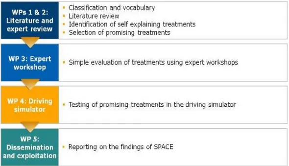
SPACE is a European project funded by the ERA-NET Roads programme “Safety at the Heart of Road Design”. The aim of SPACE is to identify self-explaining treatments that lead to the adoption of speeds that are safe and appropriate to conditions. The project is focused on rural roads with a transnational perspective. The work is divided into three parts: a literature review, expert workshops and a driving simulator study. An overview of the work packages is given in Figure 1. The present report covers the simulator study that was conducted in Work Package 4.

Figure 1: The SPACE project Work Packages

The concept of self-explaining roads (SER) is explored and discussed in the literature review that is performed in work packages 1 and 2 (SPACE Deliverable Nr 2. http://www.fehrl.org/space). The first publication on the topic was from the early 1990’s (Theeuwes and Godthelp, 1992). The original meaning of the term was described as the degree to which roads were “understandable” through the cognitive processes of categorisation and expectancy. In effect the concept of self-explaining roads was proposed originally more as a theoretical consideration than as practical guidance to road designers. Since it being proposed however, the concept has enjoyed widespread interest from practitioners, and partly because of this, the meaning of the term has broadened somewhat. The SER concept now tends to be used to refer to a wide range of psychological notions such as intuitive and understandable design, consistency, readability, and psychological traffic calming. In the literature review it was concluded that, although the concept of self-explaining roads has been widely adopted and established among traffic researchers and engineers, the evidence for the effectiveness of self-explaining road principles on behavioural outcomes is scarce. Most studies are “picture based” or done in a simulator and in some studies the self-explaining treatments are combined with other factors (e.g. road signs) that may have an influence on driver behaviour. There is little evidence that self-explaining treatments result in more homogenous speeds and there is also little knowledge

(8)

on how expectancies central to the SER concept, will differ between drivers with different levels of experience and motivation. It is suggested that a future focus of research might be to examine the relative interplay between speed differential and absolute mean speed, in an attempt to understand which of these is most amenable to influence through self-explaining road principles. The definition of self-explaining roads used by SPACE originates from Theeuwes’ and Godthelp’s meaning of the term, but it also includes some of the psychological ideas that have been added to the concept over time.

1.1 The SPACE definition of self-explaining roads

“Theeuwes and Godthelp (1992) suggested that roads are self-explaining when they are in line with the expectations of the road user, eliciting safe behaviour simple by design. This definition is largely theoretical and, where it is practically applied, it is based on road categorisation principles. In practice the term self-explaining roads has been widely adopted and has evolved to include many aspects of innovative highway engineering, including the concepts of intuitive and understandable design, consistency, readability and psychological traffic calming.”

The concept of SER and the definition adopted by SPACE was discussed in the workshops held in work package 3 (Deliverable D3 of the SPACE project, Report from expert workshop, 2011. http://www.fehrl.org/space).

In the general workshop discussions on the SER concept, some prioritized keywords were identified such as intuitive, categorization, harmonization/standardization, feedback to the

road users, road design, guide and lead.

1.2 Identification of self-explaining treatments

In work packages 1 and 2, treatments that could be considered as “self-explaining” and that could be assumed to have an influence on speed choice were identified. The identification of treatments was limited to those suitable for rural carriageways with higher volumes. In total, 72 treatments were identified and grouped according to:

• Curves

• Transitions • Intersections

• Links

Given the broad definition of SER adopted, any treatment that may be considered as self-explaining was included. The information on SER treatments was obtained from literature as well as from experts.

Treatments found for curves were chevron signing/hazard marker posts, lining, vehicle activated signs, surface treatments, SLOW markings, transverse rumble strips, optical bars, visibility and sight distance, and alignment. Treatments for transitions mostly consider gateways, i.e. transitions from rural roads to villages/towns, which usually consist of a number of features, including both physical measures (build outs, islands) and visual treatments (lining, signing and surface treatments). Intersections include cross roads, T-junctions, roundabouts and traffic signals and the treatments identified for these were additional/enhanced signing, lining/roadway markings, surface treatments, layout and junction type, and visibility. Treatments identified for links, i.e. straight road sections in between intersections and transitions, included lane width and number of lanes, surface quality and treatment, illusory lane width markings, median and edge treatments (e.g. line

(9)

markings, road studs or rumble strips), barriers, shoulder, and repetitive roadside objects (e.g. street lighting or trees). The effectiveness of each treatment is discussed and rated (low, medium or high), but it is also acknowledged that the assessment relied heavily on expert opinion rather than scientific evidence.

The effectiveness of SER treatments was further discussed in the workshops in work package 3. In the general discussions on what works, the following treatments were most frequently mentioned: road markings, road surrounding and layout (curvature, sight distance), road width/available space, guidance (barriers, chevron signing etc) and feedback (e.g. from rumble strips). Treatments that were judged as not working or not being a SER treatment were, for example, single treatments like speed limits, inconsistent signposting, and speed bumps. Based on the results from the literature review and experts it was decided that the scope of the workshops should be limited to SER treatments related to speed choice at curves and transitions. A number of films showing examples of curve and transition treatments were presented to the participants, who then discussed the advantages and disadvantages of each.

2 Aim

Work package 4 was addressed to a driving simulator test. Experiments in simulators benefit from the possibility to have a high degree of control and the possibility to build up scenarios with avoidance of confounding factors. In agreement with involved partners it was decided to focus on curves and the effect on speed in relation to the principal of treatments (consistent/inconsistent).

This study done within Work Package 4 had the main aim:

• To evaluate the effectiveness of curve treatments, in particular to determine whether a combination of treatments on curves according to their severity could help drivers correctly establish the severity of a curve in advance, and therefore adapt their speed appropriately.

3 Method

3.1 Participants

In total 35 participants aged between 20–65 years old were included (18 male and 17 female). They were recruited from VTIs register of test persons. They received a compensation of 400 SEK (approximately 42 Euro) for participating. They had an average age of 39.5 years (sd 11.7) and drove an average of 27400 km (sd 34710) each year.

3.2 Driving simulator

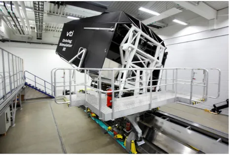
The experiment was conducted in the VTI Driving Simulator III, which is a moving base simulator (see Figure 2). The car body consists of the front part of a Saab 9-3 with a manual 5 shift gearbox. Noise, infra-sound and vibration levels inside the cabin approximate those of a modern car. The forward view is 120° x 30° from the participant’s position in the simulator.

(10)

Figure 2 VTI Driving Simulator III

3.3 Selection of scenarios

The selection of scenarios was done based on the work in SPACE work package 1 and 2. There a general identification of possible SER’s was found from the literature review, followed by a selection based on the results from workshops etc. in work package 3. Four different groups were proposed and in agreement with other partners within the consortium curves were chosen to be in focus for the simulator study. The road projected in the simulator had a lane width of 3.5 m and a shoulder of 0.75 m. The shoulder line (edge line) and the centre line was intermittent and 0.10 wide. The road had marker posts with a distance between them of 50 meters, reducing to 25 meters in the curve. The speed limit was 90 km/h.

Occasionally, there was a vehicle in the oncoming lane, but not in the curves. 3.3.1 Curves

Three types of curve were used: one slight (900 m radius), one medium (500 m radius) and one severe (400 m radius). All curves had single cross fall, meaning that the driver’s side of the road was tilt towards the ditch. The distance from the beginning to the end of the curve was approximately 280m. Only curves to the right were used.

(11)

3.3.2 Treatments Treatments included were:

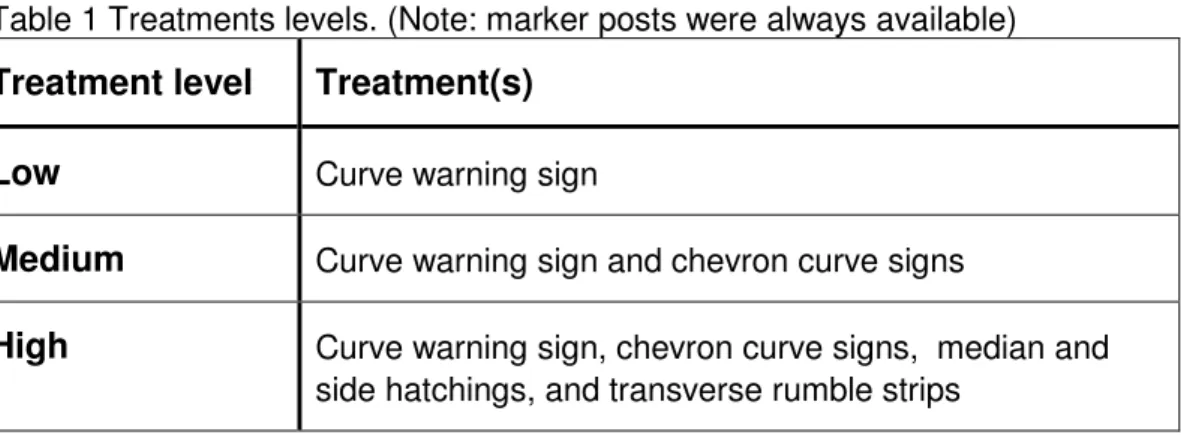
Warning sign, side hatchings, chevron curve signs and transverse rumble strips. Treatments are added in relation to the severity of the curve, see Table 1.

Table 1 Treatments levels. (Note: marker posts were always available) Treatment level Treatment(s)

Low Curve warning sign

Medium Curve warning sign and chevron curve signs

High Curve warning sign, chevron curve signs, median and side hatchings, and transverse rumble strips

The different treatments were activated sequentially. In the case of high treatment level the activation points were the following (see also Figure 5):

• v0: 350 m before curve starts (reference)

• v1: 290 m before curve starts (continuous centre line starts) • v2: 215 m before curve starts (warning sign + side hatching starts) • v3: 140 m before curve starts (transverse rumble strips starts) • v4: 20 m before curve starts (first chevron sign)

• v5: 280 m after curve starts (curve ends)

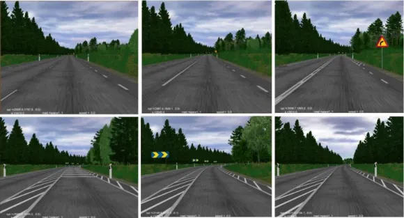
The activation points of the treatments in the low and medium levels were the same as for the high treatment level. Figure 3 show the drivers’ view of the scenario at the different points.

(12)

Figure 3 Driver’s point of view at the selected analysis point with highest level of treatment.

3.4 Consistent and inconsistent mapping

The consistency of mapping variable refers to the way in which treatment levels (low, medium and high) are applied to the different curve severities (slight, medium, sever). In the consistent mapping group, drivers experienced all slight severity curves with low treatment levels, all medium severity curves with medium treatment levels, and all severe curves with high treatment levels. Thus this condition corresponds to the spirit of the SER concept as originally defined (i.e. road situations should be obvious to the driver through consistent categorization), and this is achieved through the use of several innovative treatment types that also tend to be subsumed within the SER concept as used by practitioners. In the inconsistent mapping group there was no relationship between the severity of the curve and the level of treatment; one third of each severity of curve had low level of treatment, another third had medium level, and the final third had high level of treatment. Thus this condition did not correspond to the SER concept in terms of a consistency of categorization. Table 2 describes the different combinations, in total all drivers experience nine curves (three of each severity) in total.

Table 2 Consistent and inconsistent mapping.

Group Slight curve Medium curve Severe curve

Consistent 3: low 3: medium 3: high

Inconsistent 1: low 1: medium 1: low 1: medium 1: low 1: medium

(13)

1: high 1: high 1: high

3.5 Experimental design

As described earlier a total of 35 participants were used (18 males and 17 females). One of the participants from the consistent mapping group did only experience seven out of the nine curves due to technical problems with the simulator (#11). However, the available data for this participant was included.

Each participant drove for 46 minutes including the training and the baseline phase. The

training drive consisted of a road with one of each of the three curve severities (with

consistent level of treatment) experienced once within a four minute drive

The baseline drive used the three different curve severities, without treatment at all. During the baseline each of the three types of curves were experienced once. The baseline was in total 6 minutes.

Each experimental driving session lasted for almost 4 minutes and the driver faced 1 curve (slight, medium or severe). The selection of a specific curve for a session was done in a balanced order, see table 4. In total all participants experienced 9 curves per person.

The consistent group had the following treatments in relation to curve severity: 1=Low;

2=Medium: 3=High: (see Table 1 for details). The order of the curve/treatment for the 9 sessions was balanced.

The inconsistent group had a randomized order in relation to curve severity and treatments.

This means that 9 different orders were selected among 720 alternatives (3 curves and 3 combinations of treatments). The combination of treatments and curve are presented in Table 3.

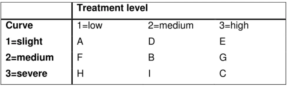
Table 3 Treatment level versus curve

Treatment level

Curve 1=low 2=medium 3=high

1=slight A D E

2=medium F B G

3=severe H I C

Figure 4 The experimental principal design

In appendix 1, Table 12 the fully session design, showing principles of the balanced and randomised session order, of the experiment is shown.

(14)

3.6 Procedure

The participants arrived at the laboratory 15 minutes before the drive started. They read the instructions together with the experiment leader and were given a verbal instruction of the scenario. “You are on your way from a weekend with some friends. You start in Vimmerby

and you are driving on road 34 on your way back to Linköping.”

The drivers signed an informed consent and completed a background questionnaire. Then they entered the simulator and the driving started. The training drive lasted for 4 minutes, followed by the baseline for an additional 6 minutes (1 slight, 1 medium and 1 severe curve, all without treatments) and then concluded with the nine curves with treatments, in the orders shown in Figure 4. In total each participant experienced 15 curves (3 during training, 3 during baseline and 9 during sessions).

After approximately 46 minutes the participants finished the driving test in the simulator and completed a post-questionnaire with questions about the experience of the test and of the consistent treatment approach. The results are used to capture the drivers experience and opinion of the treatment levels and of the concept of consistent/inconsistent treatment. This was done based on pictures exemplifying the different scenarios that they experience, see Figure 3.

3.7 Simulator data and performance indicators

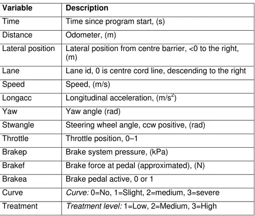
The variables that were acquired from the simulator are shown in Table 4. The sampling frequency was 20 Hz. The data from the training sessions was not analysed as part of this study.

(15)

Variable Description

Time Time since program start, (s) Distance Odometer, (m)

Lateral position Lateral position from centre barrier, <0 to the right, (m)

Lane Lane id, 0 is centre cord line, descending to the right Speed Speed, (m/s)

Longacc Longitudinal acceleration, (m/s2) Yaw Yaw angle (rad)

Stwangle Steering wheel angle, ccw positive, (rad) Throttle Throttle position, 0–1

Brakep Brake system pressure, (kPa)

Brakef Brake force at pedal (approximated), (N) Brakea Brake pedal active, 0 or 1

Curve Curve: 0=No, 1=Slight, 2=medium, 3=severe Treatment Treatment level: 1=Low, 2=Medium, 3=High

From the speed variable, instantaneous speed at six different points, v0 and v5, along the curve was determined, see Figure 5

Figure 5 The positions of the treatments along the curve. v0–v5 corresponds to the points at which speed was measured.

3.8 Statistical analysis

The key question was if a consistent treatment of curves will influence drivers to reduce their speed more when compared with an inconsistent treatment.

(16)

The design of the study was mixed; with the within-participants independent variables curve severity (slight, medium, severe) and treatment level (low, medium, high) and the between-participants independent variable group (consistent mapping, inconsistent mapping). Dependent variables were speed measurements in the different points along the curve (v0 to v5) and the average speed through the total curve (from point v0 to v5). The analyses were done both for absolute speeds and for difference in speed compared to the speed at start of the curve (v0). Four different analyses were carried out;

I. The analysis of the effects on average speed and speed at each point (v0 to v5) was done with Mixed Model ANOVA. Dependent variables were the average speed, and the speed at different points (v0 to v5) along the curve, but also the relative change in speed from the starting point to each other point (v1 to v4), for example average speed in v0 minus average speed in v5. Independent variables were consistent/inconsistent group; curve (1-3), treatment level (1-3) and order (1-9). Subject was used as random and nested on group since a person could only be either in the consistent or the inconsistent group. All interactions except for those with treatment were included in the analysis of the absolute speed levels, even though most of them were not significant. For the relative speed no interactions was significant and not included in the model.

II. It could be argued that treatment level is already by default a consequence of the grouping into consistent/ inconsistent. In order to look at the effect of the interaction between curve and consistent/inconsistent group a Mixed Model ANOVA was done without treatment as factor. Except for this dependent and independent variable were the same as in I, and interactions on second level were included.

III. In addition a Mixed Model ANOVA was used for the analysis of the combination of treatment and curve levels: A, B and C (see Table 3). The model used the same dependent variables as in I, independent variables used were group and curve. The model was based on the main factors and the interaction between group and curve, subject nested on group was used as random.

IV. In order to estimate the importance of consistent marking without an interaction of curve severity, the most severe curve was selected. A Mixed Model ANOVA was used with the same dependent variables as in I and with an independent variable for group (consistent/inconsistent) and subject as random nested on group.

(17)

4 Results

The result chapter is divided into the same four sections as the statistical analysis was presented; one dealing with the difference between the consistent and inconsistent group with treatment included as a factor (I) and one without treatment (II). An additional analysis was done with the differences between consistent treatment (A, B and C) for the consistent group versus inconsistent group (III) and finally a fourth analysis was done where we looked into differences in the most severe curve to see if the consistent marking result in higher or lower speed compare to the inconsistent marking (IV).

(I) Consistent versus inconsistent marking

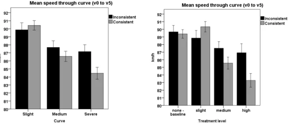
For most dependent variables there were significant effects for treatment levels, severity of the curve, order, but also for subject, see Table 5. There was no significant main effect of group (consistent or inconsistent). However, there was an interaction between curve and group (consistent/inconsistent), telling us that the consistent marking significantly reduced both the average speed among those with consistent treatment through curve and at point v2, v3 and v5. It seems that more treatments results in lower speed see Figure 6 and Table 5. The effect of curve severity was seen both in average speed and in point v4 and v5.

(18)

Table 5 Mixed model ANOVA for speed in average and at different points along the curve. Significant F-values in bold and p values in brackets.

Speed Subject (group) (Wald Z) Treatme nt (2, 336) Curve (2, 335) Order (10, 335) Group (1, 36) Group *Order (11, 335) Group *Curve (2, 335) Order *Curve (16, 339) Curve *Treatm ent (4, 335) Through curve (v0-v5) 3.82 (<0.01) 2.80 (<0.06) 16.34 (<0.01) 2.54 (<0.01) 0.19 (0.67) 1.52 (0.12) 4.77 (<0.00) 1.13 (0.32) 2.45 (0.05) V0 (Start) 3.73 (<0.01) 3.36 (0.04) 2.34 (0.10) 1.53 (0.14) 0.06 (0.81) 0.65 (0.78) 2.48 (0.09) 1.33 (0.18) 0.82 (0.51) V1 3.81 (<0.01) 6.16 (<0.01) 3.47 (0.03) 2.07 (0.04) 0.12 (0.74) 0.68 (0.75) 3.61 (0.03) 1.72 (0.04) 1.11 (0.35) V2 3.83 (<0.01) 10.45 (<0.01) 1.66 (0.19) 2.92 (<0.01) 0.17 (0.68) 0.61 (0.92) 2.34 (0.10) 1.78 (0.03) 1.74 (0.15) V3 3.78 (<0.01) 12.49(< 0.01) 3.63 (<0.01) 2.70 (<0.01) 0.09 (0.76) 1.07 (0.38) 5.45 (<0.01) 1.38 (0.15) 1.97 (0.10) V4 3.77 (<0.01) 12.51 (<0.01) 7.62(<0. 01) 4.10 (<0.01) 0.16 (0.69) 1.48 (0.14) 2.54 (0.08) 2.39 (<0.01 ) 1.03 (0.39) V5 3.81 (<0.01) 1.07 (0.34) 11.92 (<0.01) 0.79 (0.61) 0.35 (0.56) 1.15 (0.32) 5.41 (<0.01) 0.75 (0.75) 1.39 (0.24

Treatment (none, slight, medium, high); Curve (slight, medium, severe); Order (time on task 1–9); Group (consistent/inconsistent). Dependent: average speed in km/h through v0 to v5, and speed at point v0 to v5.

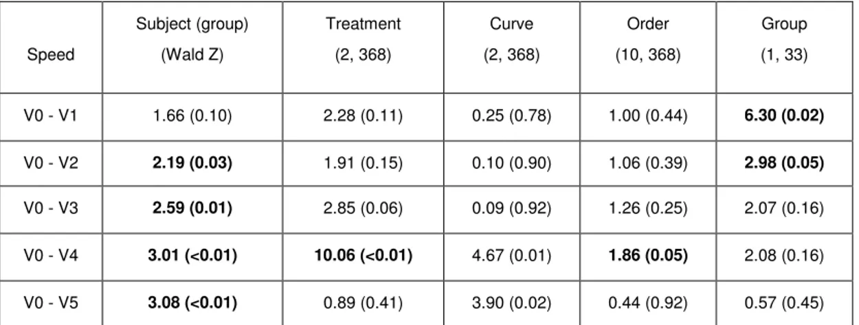
When it comes to the speed difference between starting point and each other point a significant reduction in speed was seen for the group variable (consistent/inconsistent), in point v1 and v2, in v4 for order, but also for treatment in v4 and curve in v4 and v5, see Table 6.

Table 6 Mixed model ANOVA for speed differences between at start of the curve to different points. Significant F-values in bold and p values in brackets.

Speed Subject (group) (Wald Z) Treatment (2, 368) Curve (2, 368) Order (10, 368) Group (1, 33) V0 - V1 1.66 (0.10) 2.28 (0.11) 0.25 (0.78) 1.00 (0.44) 6.30 (0.02) V0 - V2 2.19 (0.03) 1.91 (0.15) 0.10 (0.90) 1.06 (0.39) 2.98 (0.05) V0 - V3 2.59 (0.01) 2.85 (0.06) 0.09 (0.92) 1.26 (0.25) 2.07 (0.16) V0 - V4 3.01 (<0.01) 10.06 (<0.01) 4.67 (0.01) 1.86 (0.05) 2.08 (0.16) V0 - V5 3.08 (<0.01) 0.89 (0.41) 3.90 (0.02) 0.44 (0.92) 0.57 (0.45)

Treatment (none, slight, medium, high); Curve (slight, medium, severe); Order (time on task 1-9); Group (consistent/inconsistent). Dependent: difference in speed between v0 and v1; v0 and v2; v0 and v3; v0 and v4 and v0 and v5) in km/h.

(19)

ANOVA (II) Consistent versus not consistent marking without

treatment as a factor.

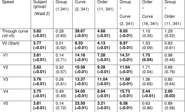
When treatment is not used as a factor in the model, group (consistent/inconsistent) as a main factor is not significant, either for average speed through curve or for speed at different points along the curve (v1 to v5), see Table 7. However, there was still an effect of order and of curve. The effect of the interaction between curve severity and consistent/inconsistent group was significant both for average speed and each point v1 to v5. This shows that there is an effect on speed due to consistent marking in relation to curve severity – the effect of curve severity is effectively increased in the consistent treatment group.

Table 7 Mixed model ANOVA without treatment as factor. Significant F-values in bold and p values in brackets. Speed Subject (group) (Wald Z) Group (1,341) Curve (2, 341) Order (11, 341) Group * Curve (2, 341) Order * Curve (16, 341) Group * Order (11, 341) Through curve (v0-v5) 3.82 (<0.01) 0.28 (0.60) 39.67 (<0.01) 4.68 (<0.01) 8.05 (<0.01) 1.10 (0.35) 1.29 (0.22) V0 (Start) 3.77 (<0.01) 0.01 (0.92) 8.33 (<0.01) 4.13 (<0.01) 8.97 (<0.01) 1.53 (0.09) 0.83 (0.61) V1 3.81 (<0.01) 0.14 (0.71) 14.18 (<0.01) 7.28 (<0.01) 14.31 (<0.01) 1.75 (0.04) 0.98 (0.46) V2 3.82 (<0.01) 0.32 (0.57) 10.58 (<0.01) 9.28 (<0.01) 11.64 (<0.01) 1.71 (0.04) 0.68 (0.76) V3 3.76 (<0.01) 0.26 (0.61) 13.37 (<0.01) 11.04 (<0.01) 11.88 (<0.01) 1.36 (0.65) 0.80 (0.64) V4 3.75 (<0.01) 0.49 (0.49) 34.05 (<0.01) 8.94 (<0.01) 15.73 (<0.01) 2.44 (<0.01) 2.00 (0.03) V5 3.81 (<0.01) 0.14 (0.72) 23.50 (<0.01) 3.21 (<0.01) 6.58 (<0.01) 0.63 (0.86) 0.89 (0.56)

Curve (slight, medium, severe); Group (consistent/inconsistent). Order (time on task 1-9). Dependent variables: difference in speed between v0 and v1; v0 and v2; v0 and v3; v0 and v4 and v0 and v5) in km/h.

(III) Comparison between combinations A, B and C for consistent

and inconsistent group

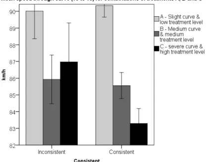
If only the combination of treatments and curve severity (A, B and C) was selected and analysed for both groups a significant effect of curve could be seen. There was no effect of group, but an interaction between group and curve for average speed, but also for speed at point v1, v3 and v5, see Table 8 and Figure 7. This results support an influence on speed due to consistent/inconsistent treatment.

(20)

Table 8 Mixed model ANOVA; Curve (slight, medium, severe); Treatment: A, B or C. Dependent variable: average speed in km/h. Significant F-values in Bold and p values in brackets.

Speed Subject (group) (Wald Z) Curve (2,174) Group (1, 174) Group * Curve Through curve (v0-v5) 3.49 (<0.01) 22.96 (<0.01) 0.38 (0.54) 3.74 (0.03) V0 (Start) 3.52 (<0.01) 6.82 (<0.01) 0.27 (0.61) 2.00 (0.14) V1 3.60 (<0.01) 11.98 (<0.01) 0.06 (0.81) 3.71 (0.03) V2 3.62 (<0.01) 11.40 (<0.01) 0.15 (0.70) 2.68 (0.07) V3 3.48 (<0.01) 13.34 (<0.01) 0.08 (0.78) 4.57 (0.01) V4 3.56 (<0.01) 21.80 (<0.01) 0.45 (0.51) 2.14 (0.12) V5 3.50 (<0.01) 15.54 (<0.01) 0.35 (0.56) 4.16 (0.02)

Curve (slight, medium, severe); Group (consistent/inconsistent).

Figure 7 Mean speed through curve (v0 to v5) comparing design A, B and C for consistent versus inconsistent marking

(21)

(IV) Severe curve - consistent and inconsistent group

The most critical situation regarding speed reduction in curve is when the curve is severe. The analysis shows that there was an effect of consistent treatment in point v4 and v5, the most critical one, see Figure 7 and Table 9. The results support an influence on speed due to consistent/inconsistent treatment.

Figure 8 Mean speed through curve (v0 to v5) in most severe curve, comparing consistent (speed 87.16 km/h; sd 7.09 km/h) versus inconsistent marking (speed 84.46 km/h; sd 6.31 km/h). Error bars

represent SE.

Table 9 Mixed model ANOVA; Severe curve; Dependent variable: average speed in km/h.

Independent is group (consistent/not consistent). Significant F-values in bold and p values in brackets.

Speed Subject (group) (Wald Z) Group (1, 33) Through curve (v0-v5) 3.19 (<0.01) 3.55 (0.07) V0 (Start) 3.00 (<0.01) 0.74 (0.40) v1 3.39 (<0.01) 2.38 (0.13) V2 3.51 (<0.01) 2.74 (0.11) V3 3.30 (<0.01) 4.54 (0.04) V4 2.81 (<0.01) 8.07 (<0.01) V5 3.03 (<0.01) 2.76 (0.11)

4.1 Drivers’ opinion

This chapter is divided into two parts; one dealing with the drivers’ opinion related to the experiment and the simulator drive, and the other one is related to the consistent treatment.

(22)

The drivers rated their experience of the test on a 7 graded scale from 1= not at all... to 7=very…. They rated the driving as quite realistic (5.30; sd 1.00), a bit boring (4.23; sd1.61) and they did not feel anxious while driving (1.54; sd 0.92), see Figure 9

Figure 9 Drivers’ experiences of the test regarding the degree of realism, boring and anxiousness. Error bars represent SE.

The drivers were also asked to rate if they found the driving demanding for the eyes, see Figure 10. In most cases they did not report high levels of complaints. Eye strain, difficulty to focus and heavy eyelids were those symptoms with highest ratings (above 2 on the 5 graded scale).

Figure 10 Drivers’ experiences of the test regarding if it was demanding for the eyes. Error bars represent SE.

(23)

4.1.3 Opinions related to consistent treatment

The participants were asked: Curves can vary in “sharpness”. How many different types of sharpness did you experience? In average the consistent group reported 3.22 curves and the not consistent group 3.47. The difference between the consistent and inconsistent group was not significant, see Table 10.

(24)

Table 10 Number of reported levels of curve sharpness during the test. P- values in brackets.

They were also asked, on a 7-graded scale if the sharpness of the curve was clear or unclear (1=unclear…7=clear), before arriving to the curve? On average the consistent group reported 5.47 and the inconsistent group 5.24. The difference between the consistent and inconsistent group was not significant, see Figure 11 and Table 11.

Figure 11 Drivers experience of the clearness of the coming sharpness of the curve. Error bars represent SE.

Table 11 Clearness of the sharpness. P- values in brackets.

Group

N Mean Std. Deviation t-test (p-value) (df 33) Group

N Mean Std. Deviation t-test (p-value) (df 33)

Consistent 18 3.22 1.77 -0.423 (0.68) Inconsistent 17 3.47 1.70

(25)

Consistent 17 5.47 1.28 0.48 (0.63) Inconsistent 17 5.24 1.56

The drivers were informed that there were three different levels of treatments before arriving at a curve and that all of them started with a warning sign for curve. They were asked to give their opinion about the information and if they had any ideas for improvements. Both positive and negative comments were given. Unfortunately it was difficult for the participants to comment on each of the presented treatments level separately, see Figure 12.

Several participants commented that they liked the treatments, but that they expected a curve that was more severe. In summary most positive comments were given regarding the warning sign, the chevrons and the hatchings (both median and centre). However, some participants comment that the hatchings and chevrons were good, but only if the curve is severe. One reason for this was that the hatching contributed to an accurate feeling of the severity of the curve.

Fewer comments were given about the transverse rumble strips. Some said that they liked them, but only if awareness was really needed.

Negative comments were given in both groups mainly regarding the placement of the warning sign. Several persons stated that it was too close to the curve. Some participants said that the hatching was too much and that there is a risk for an ‘overflow’ of information.

5 Discussion and conclusion

With the help of a moving base driving simulator the effectiveness on speed reduction of a consistent treatment regime in relation to curve severity was evaluated. One group of participants received treatments before curves that corresponded to the severity of the curve (slight curve – low treatment level; moderate curve – medium treatment level; severe curve – high treatment level); the other group had an inconsistent treatment with 9 different alternatives (combination of 3 curve severity and 3 treatment levels). In most cases there were significant effects for treatment levels, severity of the curve, order (time on task), and for subject. There was no significant main effect on group (consistent/inconsistent). However, there was an interaction between curve and group, telling us that curve severity significantly reduced the average speed among those with consistent treatment to a greater degree than for the inconsistent group. This holds true also for the speed at point v2, v3 and v5. A final

(26)

argument for the effectiveness of consistent treatment is that if only the severe curve was looked at there was a significant effect of group.

As in most studies there are also here great individual differences when it comes to performance. This is especially the case for speed. In all models subjects has been used as a random factor nested for group (consistent/inconsistent) in order to take into account these facts. Even when the speed difference was computed by using the speed at the beginning of the curve as reference still the effect of subject was significant. No matter if absolute speed or relative speed measurements were used the effect of group was significant both for average speed and for speed at most of the points along the curve. This was in line with our expectations. However, when comparing the drivers’ speeds during the baseline condition (no treatment) there were no differences in speed choice between the groups (consistent/not consistent). This indicates that the drivers before treatment started had the same preference of speed.

There is a risk that the design itself contributes to a feeling of uncertainty for the inconsistent group. They never know what will happen based on the treatments present. To test this, risk combinations A: slight curve – low treatment level; B: moderate curve – medium treatment level; C: severe curve – high treatment levels were compared for both groups. The result showed the highest reduction in speed in severe curves with high treatment level. There was no effect of group, but an interaction between group and curve. This results support an influence on speed due to consistent/inconsistent treatment – arguably the degree to which the road is self-explaining.

The most critical situation when it comes to driving through curves may occur in more severe ones. Therefore it was interesting to compare the effectiveness of a consistent high treatment level in severe curves for the two groups. The results show an average speed reduction of almost 3 km/h for the consistent group compared with the inconsistent group. This is positive and in line with our expectations.

The results from the experiment support the idea that a consistent treatment level in curves, in line with the severity of those curves, will contribute to speed reductions. This is supported since a greater speed reduction was observed in relation to curve severity with a consistent treatment level than with an inconsistent treatment level.

It is well known that the absolute level of speed in simulators is not trustworthy as a valid indicator of absolute speeds in real driving (Philip et al. 2005) and that the relative comparison is more accurate. It is difficult to say if the results in this study are externally valid in absolute terms for real driving, but it seems likely that the difference between the consistent and inconsistent treatment groups’ speed choice is reflective of a relative difference that would be expected to exist in real driving. A study from the UK is relevant here; (Helman et al., 2010) used an instrumented vehicle to examine speed choice on curves on a rural road with a 60mph speed limit, and were able to show that speeds varied with curve severity and risk, and also (independently) with the levels of treatment present. A questionnaire study within the same investigation showed the same effect of increased levels of treatment corresponding to decreasing speed. Results like this, taken with results from the current study, suggest that one fruitful way in which the self-explaining road concept can be used to improve road safety is through the use of treatment levels that vary consistently with the level of risk/severity on rural road curves.

The design of the experiment is complex, especially since both groups did not experience the same combinations of curve severity and treatment level. A consequence will be that the interaction between all independent factors is not possible to compute. This is a clear limitation, but difficult to avoid. An alternative would have been to ask the participants to come twice in order to repeat the driving session one with consistent treatment and one with inconsistent treatment. This was not possible to do due to budget limitations.

(27)

dealt with short term effects and with only familiar treatments. It is not known what the effects would be if other types of treatments were used or what impact these may have on different types of drivers. In addition it may be that different driving conditions lead to drivers adjusting their speed in a different way – for example during winter time with ice and snow on the road surface it may be even more important for drivers to be aware of curve severity. Furthermore, the variables that contribute to the objective risk present on a given curve will extend beyond severity; for example cross-fall and other idiosyncratic features on individual curves (e.g. junctions, blind entrances) might be expected to increase the fit between speed choice and risk, assuming that they can be detected by drivers (Helman et al., 2010).

A limitation with the simulator is also the effect of time on task. It is known from a large number of studies that participants will change their behavior as driving time accumulates. This is especially true if the scenario is monotonous and the risk for fatigue or sleepiness is high (Ingre et al. 2006). The analysis showed that this effect occurred in the current study; to reduce this effect in the analysis an independent factor for time on task was included in the model.

Some participants commented that even though they liked the treatments the overall impression regarding treatment did not correspond to the severity of the curve. They expected more severe curves. This may have influenced them to reduce their speed less compared to if the curve was really severe. The role of expectancy of absolute levels of severity (rather than relative ones) was not tested in the current study, and is another topic for future work.

In conclusion the results from the driving simulator study demonstrate one way to evaluate the effect of potential treatments (in this case categorized as “self-explaining treatments”) on speed choice. Furthermore, the results show that a consistent mapping of treatment levels to the severity of curves is a potential way to make drivers adapt their speed appropriately for the risk present on a given curve. For the most severe curves a consistent treatment regime (as opposed to an inconsistent one) might be expected to result in a speed reduction of around 3 km/h for the most severe curves and on the types of roads tested in the study.

6 References

Helman, S., Kennedy, J., and Gallagher, A. (2010). Curve treatments on the A377 between Cowley and Bishops Tawton: final report (PPR494). Crowthorne: Transport Research Laboratory.

Ingre, M., T. Åkerstedt, et al. (2006). "Subjective sleepiness, simulated driving performance and blink duration: examining individual differences." Journal of Sleep Research 15: 1-7. Philip, P., P. Sagaspe, et al. (2005). "Fatigue, sleepiness, and performance in simulated versus real driving conditions." Sleep 28(12): 1511-1516.

Theeuwes, J. and Godthelp, H (1992). Begrijpelijkheid van de weg (Self-explaining roads). Report IZF 1992 C-8. Soesterberg: TNO Institute for Perception.

(28)

Appendix

Table 12 The complete experimental design.

Session (1 curve per 4 minute) Training Baseline 1 2 3 4 5 6 7 8 9 Consistent Subject Sex 4min 6min 4 4 4 4 4 4 4 4 4

Yes 1 M A B C B A C C B A Yes 2 M B A C C B A C A B Yes 3 M C B A C A B A C B Yes 4 M C A B A C B B C A Yes 5 M A C B B C A A B C Yes 6 M B C A A B C B A C Yes 7 M B A C C B A C A B Yes 8 F C B A C A B A C B Yes 9 F A C B B C A A B C Yes 10 F A B C B A C C B A Yes 11 F B A C C B A C A B Yes 12 F C B A C A B A C B Yes 13 F C A B A C B B C A Yes 14 F A C B B C A A B C Yes 15 F B C A A B C B A C Yes 31* M A B C B A C C B A Yes 32* M B A C C B A C A B Yes 38* F C B A C A B A C B No 16 M B H I D F E C G A No 17 M B H I D F E A G C No 18 M A B G H I C E D F No 19 M A B G I E D C H F No 20 M C H G D B I F A E No 21 M C D I A F G B E H No 22 M D H E I B G C A F No 23 F D G B F A H E I C No 24 F E I G B C F A H D

(29)

SPACE, D4 - The driving simulator study, November 2011 No 25 F E A D I G C H B F No 26 F F D H G I A B E C No 27 F F C G H E A B I D No 28 F H C D A G E B I F No 29 F G E A I H F B C D No 30 F I H G F E B D A C No 46* M B H I D F E C G A No 53* F D G B F A H E I C