Assessments on the effects of mixing different types of GPS antennas and recievers.

(1)

Assessments on the effects

of mixing different types

of GPS antennas and receivers

Gulilat Tegane Alemu

Master’s of Science Thesis in Geodesy No. 3106

TRITA-GIT EX 08-009

School of Architecture and the Built Environment

Royal Institute of Technology (KTH)

100 44 Stockholm, Sweden

(2)

TRITA-GIT EX 08-009 ISSN 1653-5227 ISRN KTH/GIT/EX--08/009-SE

(3)

Abstract

The accuracy and reliability of the GPS system mainly depend on the GPS receiver components i.e. the GPS antenna and receiver. GPS receiver components are influenced by their types and methods of calibration. Antenna calibration determines individual GPS antenna phase variations, considering specified orientation. Different approaches of antenna calibrations provide different GPS accuracies. Therefore, in order to obtain the required accuracy from specific campaign of GPS measurements, selection of suitable antenna types and use of the same antenna and calibration method are recommended. The GPS antenna part of this thesis is focused on the effects of changing antenna orientation from originally calibrated direction (north), and then on the effects of mixing different types of GPS antennas. Trimble Compact L1/L2, Zephyr Geodetic, Leica AT502, and Ashtech 701945 E_M Rev E antennas and Trimble R7, Trimble 4000SSE, and Leica receivers are used for this investigation.

Orientation effects of antennas are studied by using two Trimble receivers and Ashtech antenna. Significant variations are observed on the horizontal vector components than on the height vector components and maximum variations are observed when rover station antenna pointing south. Form the investigation made on the effects of mixing different types of antennas great variations are observed on the height vector components than on the horizontal vector components, which range from ±2 to 4cm and variation reached maximum at Leica-to-Ashtech antenna combinations. They increase by ±1-2mm and ±2-3cm on the horizontal and on the vertical vector components, (respectively) when antenna correction factors are removed from the rover station. From the investigation made on the effects of mixing different types of GPS receivers the variations on the vertical vector components mostly lie between ±6-8mm,whereas the variation on the horizontal vector components lie between ±2mm. The result shows an agreement with previously done experiment by Freymueller (1992). Moreover, maximum variations are observed to Trimble R7-to-Trimble 4000SSE and/or Trimble R7-to-Leica receiver with Leica-to-Ashtech antenna combinations. However, effects of mixing different types of GPS receivers are smaller when comparing with the effects of mixing different types of GPS receivers. Therefore, this agreed with Völksen (2002).

Finally, this investigation has given an insight for the need of giving particular attention when mixing different types of GPS antennas and/or receivers to the same campaign, specifically, which needs greater height accuracy. The thesis also recommends that the need and importance of further research using greater numbers and types of GPS instruments using the same and/or different approach to arrive at quantifiable values of the effects on each vector components and to investigate the sources of strange results.

Keywords: GPS antenna, Antenna phase center variation, Relative calibration, NGS correction factors, GPS receiver

(4)

Acknowledgments

First, I would like to thank GOD, the one who is the engine of patient and strength. It was impossible without him to reach this stage. I would like to forward many thank to my beloved family, particularly mother Muliye-Teguye, Jerusalem and Hirut Tegane, for their encouragement and support.

I would like to thank warmly my supervisor, Prof. Dr. Lars E. Sjöberg, who leads this investigation. His inspiration and support result in to end the investigation with sound full results. I wish to express my special gratitude to Mr. Erick Asenjo, who guides technical works of the investigation. Thanks SIDA for the first ten months financial support.

(5)

Appendices

A Check for customized antenna model

B Adjustment vector components of the whole processed data

C Standard deviation values used to study effects of combining different types of GPS antenna

D Standard deviation values used to study effects of combining different types of GPS antenna

List of Figures

2.1 The GPS system measurements of arrival time for code phase, from at least four satellites in order to estimate four quantities in three dimensions (East (E), North (N), Up (U)) and GPS time (T)

2.2 Section of basic components of choke ring GPS antenna, antenna physical center, antenna reference point (ARP), L1 or L2 phase center, and height above ARP for L1 or L2

2.3 Phase center (PC), phase center offset(r), and phase center offset components (dN, dE, dU) of GPS antenna

2.4 Diagram that shows calibration method of the GPS receiver using a GPS signal simulator. A simulator generates simulated GPS antenna signal and 1pps reference

3.1 Image of observation site on the roof of L-building at KTH, which is located on Drottning Kristinas väg 30. The photo was taken while taking simultaneous observations using A-A-A antennas with S-S-S and R-R-R receivers, on stations KTH21-22-23

3.2 Configuration of the three stations, KTH21-22-23, with respect to N and approximate distances between them

List of Tables

3.1 Receiver-to-antenna combinations of R and S receivers with A, Z, C, and L antennas for simultaneous observations made by changing the patterns of antennas at KTH21-22-23 and orienting all antennas towards N. For the entire sessions, the reference station antenna is only checked for its N orientation.

3. 2 Receiver-to-antenna combinations of R ,S and Li receivers with A, Z, C and L antennas for simultaneous observations made by changing the patterns of antennas at KTH21-22-23 and orienting all antennas towards N. For the antenna at the reference station only orientation is checked at each session.

(8)

3.3 Receiver-to-antenna combinations of R and S receivers with A antennas for simultaneous observations made by changing orientation of antennas at KTH21-22-23 toward N, west (W), south (S) and east (E) respectively. At each session, reference antenna is untouched except checking its N orientation.

3.4 Receiver-to-antenna combinations for GPS observation without using beam splitter in different orientations N, W, S and E, respectively, using the same A antenna type. Antenna at control station remains untouched except checking its N orientation.

5.1 Adjustment vector components for [R-R-R] receivers with antenna type A in different orientations and NGS correction factors are applied on both stations of the baselines. Results are arranged based on antenna orientations of rover stations N, S, W and E (in that order).

5.2 Adjustment vector components for [S-S-S] receivers with A antenna type in different orientations and NGS correction factors are applied on both stations of the baselines. Results are arranged based on antenna orientations of rover stations respectively N, S, W and E.

5.3 Adjustment vector components for [R-R-R] receivers with antenna type A in different orientations when NGS correction factors are applied only at control station of the baselines. Results are arranged following the same pattern of Table 5.1

5.4 Adjustment vector components for [S-S-S] receivers with A antenna type in different orientations and NGS correction factors are applied only at control station of the baselines. Arrangements of results follows same pattern of Table 5.2

6.1 Adjustment vector components for [R-R-R] receivers with different types of N orienting antenna combinations of four consecutive sessions.

6.2 Adjustment vector components for [R-R-R] receivers with different types of N orienting antenna combinations of four consecutive sessions. NGS correction factors are applied only at control station.

6.3 N adjustment vector components (in m) and their respective standard deviations (in mm, Italic) of baseline KTH21-22 for different receiver-to-antenna combinations when NGS correction factors are applied on both stations (left) and only at control station (right).

6.4 N adjustment vector components (in m) and their respective standard deviations (in mm, Italic) of baseline KTH22-23 when NGS correction factors are applied on both stations (left) and only at control station (right) considering different receiver-to-antenna combinations

(9)

6.5 E adjustment vector components (in m) and their respective standard deviations (in mm, Italic) of a baseline KTH21-22 when NGS correction factors are applied on both stations (left) and only at control station (right) taking different receiver-to-antenna combinations

6.6 Adjustment vector components of E (in m) and their corresponding standard deviations (in mm, Italic) of baseline KTH22-23 for different receiver-to-antenna combinations when NGS correction factors are applied on both stations (left) and only at control station (right).

6.7 Adjustment vector components for H vectors (in m) and their corresponding standard deviations (in mm, Italic) taking different receiver-to-antenna combinations for all antennas oriented toward N, whereas, NGS correction factors are applied on both stations (left) and only at control station (right).

6.8 H adjustment vector components (in m) and their corresponding standard deviations (in mm, Italic), when NGS correction factors are applied on both stations (left) and only at control station (right), antennas pointing toward N.

7.1 Adjustment vector component values for GPS antenna orientation of N-N, which are taken from Appendix B for both baselines

7.2 N adjustment vector components (in m) and their corresponding standard deviations (in mm, Italic) for baselines KTH21-22 and KTH22-23, taking different receiver-to-antenna combinations when NGS correction factors are applied on both stations.

7.3 E adjustment vector components (in m) and their corresponding standard deviations (in mm, Italic) of both baselines considering different receiver-to-antenna combinations when NGS correction factors are applied on both stations.

7.4 H adjustment vector components (in m) and their corresponding standard deviations (in mm, Italic) of both baselines considering different receiver-to-antenna combinations when NGS correction factors are applied on both stations

(10)

1. INTRODUCTION

1.1 Background

GPS system is one of the most accurate and reliable positioning systems in the world. The system works all the times, everywhere, and in any weather conditions. This is the reason why it is used in a very wide area of applications like military, navigation, time dissemination, precise geodetic works, and many research areas. All these applications are based on measurements of frequency and time using GPS antennas and receivers. Therefore, accuracy and reliability of the system mainly depends on these measured parameters and measuring instruments. Beside others, any systematic errors on measurements like mixing different types of GPS antennas and/or receivers and orienting the antennas other than calibrated direction contributes significant impact on accuracy and reliability of the system. It is also believed that the effects of GPS receivers are less crucial than the antennas (Völksen, 2002).

In the whole process of measurements the GPS antenna filter, amplify, and convert the incoming signal from satellite into an electrical signal at its phase center (PC), the receiver then determines coordinates of this PC. More remarkably, the location of the antenna PC is different for different types of antennas (Mader, 2002) and varies based on elevation angle and azimuth of observation and strength of incoming signal (Gurtner at al., 1989). As a result, antenna calibration is used to determine the best general phase corrections for a given antenna model (Rothacher and Mader, 1996). Different organizations are participated in these operations, and National Geodetic Survey (NGS) is one of them that provides complete summary of all calibration results free of charge.

Antennas are traditionally calibrated for north (N) orientation using reference antenna. Despite their similarities, when taking GPS observation both antennas of a baseline must be oriented to the same direction, preferably towards N. If these conditions are not satisfied, there could be systematic effects on horizontal components, and the worst condition occur when one antenna points to N and another is to south (S) (or 1800 difference between them). However, Bányai (2005) pointed out that the effect is in height components too.

In principle, it is also not recommended to mix different types of antennas to avoid systematic errors come from instruments, since different types of antennas exhibits different phase variations (Mader, 2002). There are small phase canter variations (PCVs) within one-antenna types as well (Schmid et al. 2004). In line with this, according to Freymueller (1992) when mixing different types of GPS receivers uncertainties of 2-3mm in the horizontal components and more than 8mm in the vertical components have been observed for short baselines.

However, due to instrument unavailability, financial matters, technical and other considerations combination of different types of antennas and/or receivers might be taken as a solution. This clearly shows that how the knowledge on the effects of mixing

(11)

different types of GPS antennas and/or receivers with the effects of antenna orientation is significant.

In this study, emphasis has mainly been given on the effects of antenna orientation and mixing different types of antennas and/or receivers. Assessments of the thesis have been divided into eight chapters and three parts. The first part (Chapter 2) is mainly devoted to theoretical reviews of the study, whereas, the second part (Chapter 3 and 4) gives brief information about session planning and the GPS data collection and analysis. Finally, the third part (from Chapter 5 to 8) shows the effects of antenna orientations, mixing different types of antennas and receivers, and recommendations for future works.

Chapter 2 is mainly devoted on theoretical reviews of calibration and mixing different brands of GPS antennas and receivers. After a review on fundamentals of the GPS system, discussions will be made on antennas and receivers. Antenna phase center offset basic equations are derived and Phase Center Variation (PCV) is explained briefly. Antenna calibration portion covers: aim of antenna calibration, methods used to measure the phase patterns, NGS antenna calibration procedures, use of identical calibration methods and their drawbacks. Effects of antenna orientations and mixing different types of them with sources of errors and some remarks will be explained. Types of GPS receivers, measurement uncertainties of them with the need and methods of their calibrations come prior to the discussion on mixing different types of GPS receivers.

Chapter 3 is devoted on session planning of the study. Beside selection of instruments and GPS data collection, it covers how synchronization of observations have been made using approximately the same session length, elevation mask, time interval, observation time, and receivers and antennas via out. Creation and test of customized antenna for Ashtech 701945 E_M Rev E, and approaches on determination of representative data, analyzing of them, and arrangement of obtained results will be explained at great depth in Chapter 4.

Assessments on the effects of GPS antenna orientations, mixing different types of GPS antennas and receivers will be explained in Chapter 5, 6 and 7, respectively. Following the same fashion, analyzed results will be displayed in tables, discussed and concluding remarks will be drawn. Particularly for the later two chapters assumptions will be developed and discussions will be made for separate adjustment vector components. Finally, recommendations for future works are pointed out in Chapter 8.

1.2 Problem statements

Now-a-days the GPS system is the most precise and commonly used positioning system worldwide. Its weather, place, and time independent application makes the system more popular. The GPS system is composed of four components: the satellites, the control stations, the International GPS and Geodynamic Service (IGS) stations (not regular), and the GPS receivers (Sjöberg, 2006). The last component consists of a computer to store and process the signals coming from the antenna. The GPS of antenna is used to convert

(12)

the energy in a time-varying electromagnetic wave into electronic current, which is connected to some external electronic circuits, called the GPS receiver.

GPS antennas are manufactured by different manufacturers; hence, they are available in many different brands. Besides, systematic errors may come from manufacturing of the antennas. Therefore, antennas are calibrated by considering the systematic errors and external factors that influence their function. For relative antenna calibration method, test antenna has been calibrated relative to control antenna under defined conditions for N orientation. The first aim of this study is to check the effects of antenna orientations on vector components using the same measuring environment.

Regardless of different antenna types, many organizations are involved in antenna calibrating operation. This implies that antenna precision depends on both antenna type and its method of calibration. These days, for precise geodetic applications like geodetic control and deformation monitoring, an advanced choke-ring antenna is used because of its configuration that allows better reception of low elevation angle GPS satellites and improved multipath rejection. As a trend, it is not recommended to mix different types of antennas for the same campaign. However, there are economic, instrument availability, and technical factors that force the use of mixed brands.

In 2004, significant biases were observed, which should not exist according to the manufacturer, when taking GPS measurements by mixing two types of antennas (Dornie Marolin T and Trimble choke-ring antennas) in the Swedish Nuclear Fuel and Waste Management Company (SKB) deformation network outside Oskarshamn (Sjöberg et al., 2004).

The second aim of this investigation is to study the effects of mixing different types of GPS antennas and to point out the most affected vector components and the worst antenna combinations. The investigation uses relative antenna calibration method, two short baselines comparisons, four different antenna types, beam splitters for the GPS data collection and the effects of antenna orientation.

Likewise antennas, there are different types and calibration methods of GPS receivers. Due to differences in performance, under the same location, satellite constellation, and measuring environments the same types of receivers provide different frequency values. Therefore, it is clear that mixing different types of GPS receivers affects the precision of measurement; however, this is less crucial (Völksen, 2002). The final aim of the investigation is thus with the intention of evaluating the effects of mixing different types of GPS receivers. This evaluation has considered different types of receiver-to-receiver combinations and effects of mixing different antenna types.

(13)

2. THEORETICAL REVIEWS ON CALIBRATION AND MIXING

DIFFERENT TYPES OF GPS ANTENNAS AND RECEIVERS

2.1 Fundamentals of GPS system

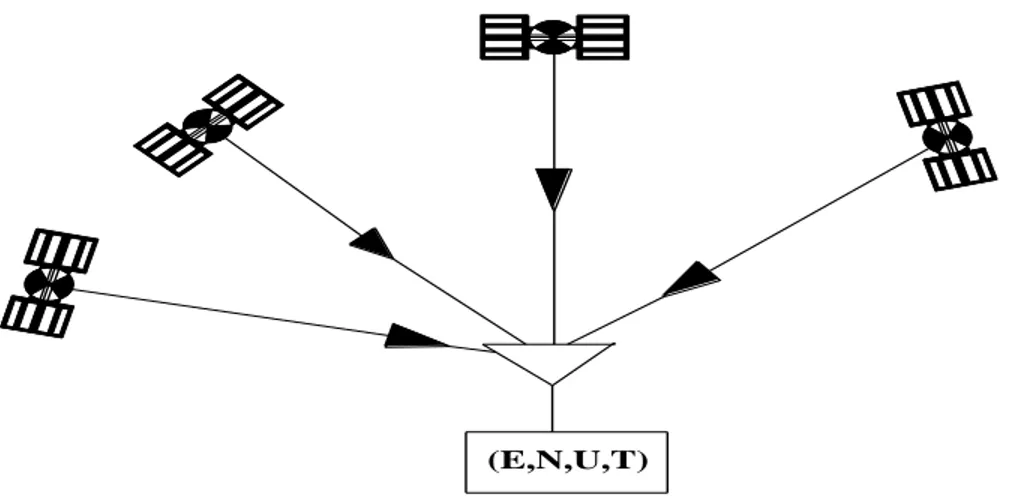
GPS is founded by and controlled by the U. S. Department of Defense (DOD). Besides its primary military target in the present time GPS is the best system in the areas of navigation, positioning, time dissemination, and other researches. GPS provides specially coded satellite signals that can be processed in a GPS receiver, enabling the receiver to compute position, velocity and time. At least four GPS satellite signals are required in order to perform such operations and the whole system can be demonstrated in Fig.2.1 below.

(E,N,U,T)

Figure 2.1 The GPS system measurements of arrival time for code phase, from at least four satellites in order to estimate four quantities in three dimensions (East (E), North (N), Up (U)) and GPS time (T).

Position is determined from multiple pseudo-range measurements at a single measurement epoch. The pseudo range measurements are used together with space vehicle (SV, called satellite) position estimates based on the precise orbital elements (the ephemeris data) sent by each SV. This orbital data allows the receiver to compute the SV positions in three dimensions at the instant they sent their respective signals.

These days the whole process of the GPS system is composed of four components. These are the satellites (SVs), the control stations, the International GPS and Geodynamic Service stations (IGS stations) and the GPS receivers (Sjöberg, 2006).

There are 32 SVs at 20200 km altitude in six equally spaced orbital planes at 550 inclinations from equatorial plane that send radio signals from space. Control stations are five in number, with the main station located in Colorado spring, their main tasks are tracking the SVs and updating the orbital information, correcting SVs clock and synchronizing them with GPS time, checking SVs health, and other system adjustments. IGS station consists of a global network of high quality GPS sites (determined by SLR

(14)

and/or VLBI), equipped with permanently observing GPS receivers, which data is continuously sent to the IGS data centers for processing of various types of accurate orbital data (Sjöberg, 2006). The last component consists of the GPS receivers and antennas with user community. GPS receivers convert SV signals into position, velocity, and time estimates. This component is the main objective of the thesis and this chapter (in particular), first on the effects of GPS antenna orientation and mixing different types of GPS antennas and then on the effects of mixing different GPS receiver types.

2.2 GPS antenna

GPS antenna is the main component of the GPS system that is used to filter, amplify, and down-convert the incoming signal into an electrical signal that can be processed by the receiver. The receiver then determines the coordinates of the electrical phase center (PC) of the antenna. Since antenna is used for receiving GPS signal, phase center is the point at which electromagnetic wave energy is transferred to the antenna i.e. an effective collecting point of the radiation. This point may always not be a physical center of the antenna. Fig.2.2 demonstrates a section of the basic components of GPS antenna of choke-ring model.

L1 phase center Antenna physical center

Height above ARP for L2 Height above ARP for L1 Antenna reference point (ARP)

L2 phase center

Figure 2.2 Section of basic components of choke ring GPS antenna, antenna physical center, antenna reference point (ARP), L1 or L2 phase center, and height above ARP for L1 or L2.

2.2.1 Phase center offset

This is the constant vector between the phase center and an external Antenna Reference Point, ARP (which is usually the base of the antenna mount).The main phase centre offset component is vertical (up, dU) but there are also small horizontal offsets (north and east, dN and dE). In an antenna, there are two-phase centers, one for the L1 frequency and the other for L2, but each phase center has a different offset. Fig.2.3 shows the phase center, phase center offset and phase center offset components.

(15)

Figure 2.3 Phase center (PC), phase center offset(r), and phase center offset components (dN, dE, dU) of GPS antenna.

2.2.2 Basic relations

As a first step, in order to define the three vector components of antenna offset (r), let us consider the convention that antenna physical center as an origin, the N-axis points towards north, E-axis point towards east, and U-axis along zenith direction. For N, E, and U components of dN, dE, and dU an antenna-offset components are related by (refer Fig.2.3): cos cos r dN (1) sin cos r dE (2) sin r dU (3)

where α, and ε are azimuth and elevation angles respectively.

Considering Fig.2.3, when N-axis rotates by angle (let theta, θ) about U-axis in clockwise direction from N towards E, one can derive relationships for antenna offsets like:

sin ' sin cos ' sin cos ' r dU dE dN dN dN dE dE (4)

where dE,, dN and ' dU are respective vector components after rotation. Rotational ' matrix can be written as:

dU dN dE dU dN dE 1 0 0 0 cos sin 0 sin cos ' ' ' (5)

(16)

1 0 0 0 cos sin 0 sin cos U R (6)

where R is the axis of rotation matrix for a rotation about the U-axis. From Equation _U (6) the rotation matrix shows that only horizontal components are subjected to change when N-axis rotates about U-axis.

In principle, antenna height is measured vertically from the station marker to the ARP for each antenna. Therefore, the offset from the ARP to the phase canter has been added to the ARP height in order to get the height of the phase center above the ground marker. However, antenna phase center consists of this offset and a variable value as a function of azimuth and the elevation of the incoming signal (Gurtner et al., 1989). This implies that, the offsets and the phase center variations (PCV) together define the reception characteristic of an antenna.

2.2.3 Antenna phase center variation (PCV)

Antenna phase variation is a variation of the antenna phase center beyond the antenna offset. Different antenna types exhibit different phase variations Mader (2002). The GPS antenna phase center shifts in position with varying observed elevation angle and azimuth to the satellite. This shift is expressed by mean phase center offsets and by phase and amplitude patterns for L1, L2, and L3 (ionosphere free combination) (Schupler and Clark, 1991, Wu et al., 1993). Based on the frequency of received signal the shift is measured in the order of several centimeters (Schupler et al., 1994). Lack of determining the exact PCV was the vital source of errors on the study of mixing different types of receivers (Freymueller, 1992). Thus, PCV problem is significant for applications requiring the highest attainable precision from GPS.

Therefore, it is necessary to know the exact position of the phase center of the transmitting as well as of the receiving GPS antenna (i.e. offsets and PCV) in order to achieve high-precision GPS results, which means antenna calibration.

2.2.4 Antenna calibration

2.2.4.1 Aim of antenna calibration

The main goal of antenna calibration is to determine the best general phase corrections for a given antenna model with the understanding that there are specific site influences, which can modify the pattern and introduce additional measurement errors, as shown in Rothacher and Mader (1996). This can be done in various ways.

(17)

2.1.4.2 Methods to measure the phase patterns of the GPS antenna

There are principally two ways used to measure the phase patterns of GPS antennas. The first is in an anechoic chamber (Schupler and Clark, 1991) and the second is in the field using actual GPS signals. For the field measurements there are two types of calibrations, one using antenna rotations and the other using relative differences with respect to a reference antenna (Rothacher et al., 1995).

In practice, relative antenna calibrations are perfectly acceptable over shorter baselines (less than several hundred km) because the elevations from each antenna to the same satellite are not significantly different. However, on longer baselines (greater than a few thousand km) the curvature of the earth causes the elevations to the same satellites to be significantly vary; hence, knowledge of the absolute PCV becomes essential (Mader, 2006).

National Geodetic Survey (NGS) is a well-known organization that performs antenna calibration and provides complete summary of all calibration results. This thesis has used the NGS relative antenna calibration model.

2.2.4.3 The NGS relative antenna calibration procedure

According to the NGS relative antenna calibration procedure, the test range consists of two stable 6in. diameter concrete piers rising about 1.8m above the ground. They are separated by 5m, located in a flat grassy field and lie along N-S line, and on top of them antenna-mounting plates are permanently attached. The reference (on the N pier) and test antennas are connected to receivers, which are set to track an elevation mask of 100. The reference antenna is the same for all tests. A Rubidium oscillator is used as an external frequency standard for both of the receivers.

2.2.4.4 Use of identical calibration method

Different antenna calibration methods are performed relative to a specific antenna and have been done under identical conditions i.e. consistent set of measurements. This infers that, different calibration techniques have different sources of systematic error that may not cancel out when using results from different schemes. Thus, it would not be advisable to use the results from different calibration techniques (Mader, 2002).

2.2.4.5 Drawbacks of relative calibration

A database of relative antenna calibration that is generated by Mader covers a large variety of different antenna types, updated regularly, and accessed freely to everyone. However, Völksen (2005) has pointed out the following as the drawbacks of the method:

 Corrections are dependant on a reference antenna;

 Estimation of PCV at low elevations is not possible due to much noise and strong multipath signals;

(18)

 Observation is never completely free of multipath, which has an impact on the calibration results; and

 The satellite constellation at the location of calibration might not cover evenly the hemisphere of the antenna.

In 1994, the first absolute field calibration method was developed by Schupler and Clark by making use of an anechoic chamber. The main purpose of this method is in order to estimate antenna PCV independent of a reference antenna by eliminating effects of multipath.

Nowadays, relative PCV calibration models are commonly used as standard GPS processing method, but there is no guarantee that they are applicable for different circumstances. Therefore, the only solution would be a transition from relative to absolute phase center corrections (Schmid et al. 2004).

2.2.5 Effects of GPS antenna orientations

As a traditional procedure for relative GPS antenna calibration (by NGS), both reference and test antennas were oriented toward N. This clearly shows that, at the ends of a certain baseline both antennas must be oriented in the same direction, preferably toward N. However, when one or both of the antennas are oriented other than N, it is clear that the magnitude of the horizontal offset is subjected to change.

Suppose that the same network is measured simultaneously on two consecutive days under the same satellite configuration, but by rotating one of GPS antennas from the N to the S direction in the second session. This gives rise to the same horizontal mean phase offset but has a different sign. Consecutively, rotation of the antenna in the horizontal plane does not cause a change in the vertical components of the measured baselines. However, the vertical components cannot be separated from the baselines; therefore, they will bias the vertical components of the position vectors (Bányai, 2005).

2.2.6 Mixing different types of GPS antennas

The problem of mixing different types of GPS antennas was recognized in the early years of geodetic GPS applications, at the IGS Analysis Center Workshop in Silver Spring, in 1996. In order to handle this, several antenna calibration campaigns were organized using a local network of stations separated by some tens of meters controlled by precise geodetic measurements (Seeger et al. 1992). According to these assessments, the differences between the nominal and the estimated mean phase centre offsets were reduced to less than 1 cm (Gurtner et al. 1989). The special effect of different antenna phase patterns was recognized after the International GPS Service (IGS) Test.

Besides small PCVs within one antenna type (Schmid et al. 2004), Mader (2002) points out that different antenna types exhibit different phase variations. According to him, precise knowledge of phase patterns is essential. Phase patterns are normally defined as the azimuth and elevation dependence to be added to the average phase canter offsets.

(19)

Therefore, the sum of the mean phase offset and pattern gives the signal path delay for given satellite elevation and azimuth. This knowledge is (particularly) important for those applications that require high resolutions in the height components (Stewart, 1997).

These height components are usually measured by the user to some point on the antenna using an internal correction to the location of the phase center specified by the manufacturer. The correction is automatically applied in either the receiver firmware or the post-processing software. Hence, it is logical to assume that there are some systematic errors from manufacturing, calibration, or processing when mixing different antenna types.

According to Völksen (2002), mixing of receiver types soon became less crucial but mixing of antenna types of different design remained as a serious problem. UNAVCO Annual Report (1996) has also specified that the effects can be as large as 10cm in the vertical and 1cm in horizontal baseline components. However, the effect in the vertical is below 5mm without tropospheric scale and in the cm-range with tropospheric scale with a combination of different antenna types and absolute PCV calibration (Menge et al, 1998). This implies that, the effects of mixing different antenna types are somehow significant for those of relatively calibrated antennas without trophospheric scale.

2.2.6.1 Sources of antenna mixing error residual

Antenna mixing error residual has several possible sources. These mainly include the following two (UNAVCO 1996 Annual Report):

1. Calibration antenna operated on ideal low multipath environment whereas field observations are influenced by multipath ,and

2. Monument effects and differences in phase patterns between mixed antennas can be easily confused with tropospheric delay, particularly at low elevation angles.

Multipath and antenna environment creates significant impact on the GPS results. These may include; any multipath producing or absorbing materials around the antenna, snow on the antenna, wet ground after rainfall, height of antenna above the ground, the monument design, the antenna ground plane, and radoms. Thus, it is necessary to consider field tests while performing phase center variation models.

Simultaneous use of different calibration methods and/or small variations of PCVs within one antenna type are considered as a source of antenna mixing error residual (Schmid et al. 2004).

2.2.6.2 Remarks on mixing different types of antennas and calibration methods When mixing different antenna types and/or calibration methods, one has no guarantee to obtain height estimates with sub-centimeter accuracy, even by correcting the observations for antenna specific phase center variations (as available at the IGS Central Bureau). The conclusion and the recommendation that follows is that, whenever possible, for precise

(20)

site coordinate determination the same antenna types should be used for all sites. In addition, the antenna setup (including antenna, Radom, orientation, environment) should not be changed unless it is necessary (Mader, 2002). It is also a new insight to use Antenna and Multipath Calibration System (AMCS) for characterizing site-specific GPS phase measurement errors as proposed by Hannover group (IGS workshop, 2002).

2.3 GPS receiver

GPS receiver is one of the four GPS system components, which consists of a computer to store and process the incoming signal from the circum-polar antenna. Normally the receiver is equipped with a keyboard and a screen to allow various operations to the operator in the field (Sjöberg, 2006). Its characteristics depend on the applications for which it is designed; either as military receivers, commercial receivers (for navigation), or receivers used for time and frequency metrology.

Basic frequency (10.23 MHz) of the GPS system is multiplied by 154 and 120 in order to get carrier frequencies of L1=1575.42MHz and L2=1227.60MHz, with respective wavelengths of 19cm and 24.4cm. Whereas, C/A- and P-code signals are those signals that correspond to 300m and 30m wavelengths of basic frequency respectively. Different GPS receivers can receive one or more types of GPS signals.

2.3.1 Types of GPS Receivers

GPS receivers can be categorized into different classes based on the type of signal that they receive and on their specific applications (viz. navigation, geodetic, and military). They are divided into four types based on the signal they receive (Sjöberg, 2006):

1. C/A-code pseudo-range receiver: navigation type, hand-held, only a few channel; 2. C/A-code carrier phase receiver: one-frequency receiver;

3. P-code carrier phase receiver: L1 and L2 signal precise geodetic receiver; and 4. Y-code carrier phase receiver: military type and can derive the P-code,

anti-spoofing (AS) invoked.

2.3.2 Measurement uncertainties of GPS receivers

The main sources of uncertainties in the GPS measurements are the GPS receiver position error, the orbital error, the satellite and receiver clock errors, the ionospheric and the tropospheric delays, the receiver internal delay, the satellite antenna and antenna cable delay, the receiver noise and the multipath error.

Measurement uncertainty of the majority of commercial GPS receivers varies from 10-11 to 10-13 by the frequency scale, and from 100ns to 50ns by the time scale, depending on the receiver design. The frequency uncertainty for a GPS receiver is larger than Cs-standard by 2-3 orders within a short-time interval (1–1000s) and by one order within a long-term interval of about one week. Time scale biases the GPS receiver from the Universal Coordinated Time (UTC), and it can be in order of microseconds. Therefore, the GPS receiver calibration against the primary time and frequency standard (the

(21)

Cs-atomic clock traceable to UTC) is of great importance and implies the calibration of both output frequencies and time scale.

2.3.3 Need of the GPS receivers calibration

Two GPS receivers always yield different frequency results (due to their performance differences) even when they are connected to the same antenna, at the same location and the same measuring environment. These uncertainties may come from receivers’ noise and instability of internal oscillators, software errors, time delay in antennas and antenna cables and receivers’ internal delay. Therefore, calibration of GPS receiver is of great importance in order to determine (Goldovsky and Kuselman):

 Frequency deviation from its nominal value and its uncertainty;  The GPS receiver second bias from the SI second; and

 The GPS receiver time scale deviation from the UTC.

Summing up, the GPS receiver calibration implies the calibration of output frequencies and the calibration of time scale. The frequencies calibration is performed through comparison of one pulse per second (1pps) with the corresponding reference frequency Cesium atomic standard. The time interval counter measures the time differences between calibrated and reference signals.

2.3.3.1 GPS receiver calibration method

The calibration of the GPS receiver is accomplished with a GPS signal simulator. The simulator generates two signals: a simulated GPS antenna signal and a 1pps reference signal (White et al., 2001). The receiver is connected to the simulated antenna signal and the time determined by the receiver is compared with the time of the simulator reference (see Fig.2.4).

(22)

DATA 1 PPS DATA 1 PPS L BAND TIME INTERVAL COUNTER RECEIVER ANTENNA SYSTEM SIMULATOR

Figure 2.4 Diagram that shows calibration method of the GPS receiver using a GPS signal simulator. A simulator generates simulated GPS antenna signal and 1pps reference. The time determined by the receiver and the simulator reference has been compared after the receiver connected to the simulated antenna signal.

The simulator is calibrated first by connecting a high-speed digital scope to both outputs of the signal simulator. Calibration of the simulator is defined as the delay of the null in the envelope of GPS signal for the 1pps reference. In some cases, an antenna system is placed between the simulator and receiver. The combination can be calibrated as a whole or in parts. If in parts, the delay of the antenna system is measured with a network analyzer. The absolute calibration of the receiver is defined as the delay of the receiver tick from the simulator tick less the simulator calibration and less the antenna system delay (Landis and White, 2002).

2.3.4 Mixing different types of GPS receivers

Any GPS survey generally uses two or more receivers. Moreover, the same types of receivers under the same condition of measurements provide different frequency values. In spite of the above fact, the normal trend is to use the same brand of receivers for data collections and then to process through software supplied by the same manufacturer.

However, for precision demanding geodetic works, mixing of different brand receivers with the same or different antennas and/or software supplier can be performed from economic, availability, and/or other technical point of views. Völksen (2002) pointed out that mixing of receiver types soon became less crucial when comparing with mixing of antenna types of different design. On the other hand, according to Clynch et al. (1989) main technical factors to be considered while mixing different GPS receivers of the same and /or different manufacturers are:

1. Data format: when different types of receivers are mixed, a standard data exchange format commonly understood by users is necessary. Receiver Independent Exchange Format (RINEX) was proposed to do so (Gurtner et al.,

(23)

1990), but problems on RINEX was identified by Hendy et al. (1993). It requires clear understanding of how each manufacturer applies clock errors and time tag.

2. Receiver clock and time tags: Rizos (1994) pointed out three issues:

a. All receivers should take observations to common-view satellites at epochs which are within 30 milliseconds (to cancel out satellite errors in between receivers differencing);

b. Receivers should be synchronized with each other at microsecond level to ensure that all observation time tags are consistent with each other; and

c. All receivers should be externally synchronized to the satellite ephemeris at microsecond level (in general the GPS time).

3. Antenna phase center: it consists of an offset value and a variable value as a function of azimuth and elevation of the incoming signal (GÜrtner et al., 1989).

The offset values are normally made known by the manufacturer, thus necessary corrections can be applied.

Tests were conducted on the Ecuador 1990 GPS campaign (February 1990) to measure crustal motion and simultaneously to determine intrinsic bias introduced in baseline solutions by mixing different GPS receivers. TI-4100 and Trimble 4000SDT Geodetic GPS receivers were used. The data were analyzed using the GIPSY software developed at the Jet Propulsion Laboratory (JPL) of California Institute of Technology. The formal uncertainties are 2-3mm in the horizontal components and 7-8mm in the vertical component for 25m baseline, whereas, 2mm and increased by a factor of four for 28km respectively. The vertical difference is may be because of the need to estimate the tropospheric delay independently at each site. At the end of his survey, Freymueller (1992) arrived at the conclusion that any errors in the phase center locations used in the analysis will bias solutions for mixed-receiver baselines.

Therefore, while studying the effects of mixing different types of GPS receivers, it is the key to consider the types of antennas that are used and/or their nature of PCV, since the electromagnetic behavior of antennas is not homogenous. Moreover, considerations have to be given:

 For systematic errors on manufacturing and calibration of different types of receivers;



On types of receivers and types of the signal that they receive; and



On conversion of observation data and use of appropriate software to analyze the baseline.

(24)

3. FIELD OBSERVATIONS

For this particular study GPS data were collected by taking two different short baselines. According to the requirements of the investigation and availability of instruments different receiver-to-antenna combinations are considered at session planning stage.

3.1 Session planning

Session planning of the GPS data collection is made to have optimum conditions of survey operation by answering questions like, the best time regarding satellite visibility, Dilution of Precisions (DOPs), approximately the same satellites constellation, receiver-and-antenna arrangement, and others.

Bearing in mind the subject matter of the thesis (at this stage), the following points are tried to be considered to synchronize observations. These are:

 Taking the same receivers and antennas at respective stations through out the observation;

 Tracking all the observations approximately at the same time (afternoon), to have relatively the same satellite constellation; and

 Recording the data at the same elevation mask (of 100

), at the same time interval (of 15 seconds) and at the same length of session (nearly 1 hour).

Moreover, considerations are given to keep control station antenna untouched (except checking its orientation) for all the observations and to take redundant data.

For carrying out of GPS observations, the roof of L-building at KTH, which is located on Drottning Kristinas väg 30, is used. This location contains three stations (hereafter KTH21, KTH22, and KTH23) and they are placed on the wall. The coordinates of the middle station are known and taken as a reference station.

Selection of GPS instruments for the observations was primarily made based on the need for the thesis, and then by considering availability of them at the Division of Geodesy. Thus, Trimble Compact L1/L2, Zephyr Geodetic, Leica AT502, and Ashtech 701945 E_M Rev E (henceforward C, Z, L and A, respectively) antennas and Trimble R7, Trimble 4000SSE, and Leica (henceforth R, S and Li, respectively) receivers are planned to be used.

Consideration is given for different arrangements of GPS to-receiver, receiver-to-antenna, antenna-receiver-to-antenna, and antennas in different orientations. For simultaneous observations with and/or without beam splitters on the three stations (in future KTH21-22-23), the following arrangements (see Table 3.1, 3.2, and 3.3) are made.

(25)

Table 3.1 Receiver-to-antenna combinations of R and S receivers with A, Z, C, and L antennas for simultaneous observations made by changing the patterns of antennas at KTH21-22-23 and orienting all antennas towards N. For the entire sessions, the reference station antenna is only checked for its N orientation.

Station KTH21 KTH22 KTH23 Antenna orientation for KTH21-22-23 Receiver combinations R R R S S S Antenna combinations A A A N-N-N Z A Z N-N-N C A C N-N-N L A L N-N-N

Table3. 2 Receiver-to-antenna combinations of R ,S and Li receivers with A, Z, C and L antennas for simultaneous observations made by changing the patterns of antennas at KTH21-22-23 and orienting all antennas towards N. For the antenna at the reference station only orientation is checked at each session.

Station KTH21 KTH22 KTH23 Antenna orientation for KTH21-22-23 Receiver combinations R R R Li S Li Antenna combinations A A A N-N-N Z A Z N-N-N C A C N-N-N L A L N-N-N

Table 3.3 Receiver-to-antenna combinations of R and S receivers with A antennas for simultaneous observations made by changing orientation of antennas at KTH21-22-23 toward N, west (W), south (S) and east (E) respectively. At each session, reference antenna is untouched except checking its N orientation.

Station KTH21 KTH22 KTH23 Antenna orientation for KTH21-22-23 Receiver combinations R R R S S S Antenna combinations A A A N-N-N A A A W-N-W A A A S-N-S A A A E-N-E

(26)

Table 3.4 Receiver-to-antenna combinations for GPS observation without using beam splitter in different orientations N, W, S and E, respectively, using the same A antenna type. Antenna at control station remains untouched except checking its N orientation.

Station KTH21 KTH22 KTH23 Antenna orientation for KTH21-22-23 Receiver combinations R or R or R or S S S Antenna combinations A A A N-N-N A A A W-N-W A A A S-N-S A A A E-N-E 3.2 GPS data collection

For carrying out of GPS data collections, the stability of each station is checked and the screws mounted on top of the three poles fit tightly. After making the stations stable enough and ready, GPS antennas were mounted over the poles, receivers were on, the satellite cut-off angles and the sample intervals were set to 10 degrees and at 15 second (respectively), finally collection of GPS data is started. Simultaneous data are collected at each station for about 1 hour session.

After arranging instruments and conducting an observation, photos were taken for observation site. GPS observation shown in Fig.3.1 is an image while taking simultaneous observation using A-A-A antennas with S-S-S and R-R-R receivers, on stations KTH21-22-23.

Figure 3.1 Image of observation site on the roof of L-building at KTH, which is located on Drottning Kristinas väg 30. The photo was taken while taking simultaneous observations using A-A-A antennas with S-S-S and R-R-R receivers, on stations KTH21-22-23.

(27)

N 5.940m 3.484m KTH22 kth23 kth21 Figure 3.2 Configuration of the three stations, KTH21-22-23, with respect to N and

approximate distances between them.

All the observations are performed according to the plan (see Tables 3.1 to 3.4). When simultaneously using only A antennas at all the stations, those antennas that were used on rover stations are first centered toward N, then W and S, and finally towards E orientation at each session, respectively. Whereas, when different types of antennas are used, those antennas that were used on rover stations are centered and oriented toward N and replaced by another at the end of each session. However, an antenna that was used at control station was still untouched except checking its orientation all the time. Simple compass was used for these operations.

When the session is done for particular antenna-to-receiver combination, the receivers were switched off and the antennas were rotated or replaced and adjusted for the next session.

Whichever of using the same type of antenna on different orientations or using different types of antennas one after the other at each session, one-day GPS observation consists of four sessions. At the end of each day sessions, collected data were transferred, checked and arranged for analysis.

(28)

4. GPS DATA ANALYSIS

GPS data are analyzed by making use of Trimble Total Control (version 2.73) software. While analyzing, the Swedish National Reference System (SWEREF99), NGS ant_info.003 antenna model, and L1 frequency measured to Antenna Phase are used.

Based on the application of NGS correction factors, the whole analysis are made in two different ways. Firstly, by applying the correction factors on both stations of the baseline and then removing them from rover station. The later is used when analyzing GPS data on the effects of mixing different types antennas.

Moreover, those GPS data, which were collected by Li receivers are converted into RINEX format (using version 3 SKI-Pro software), to avoid systematic errors result from using different software. Moreover, the software adopted for this particular thesis has no antenna model for A, which is less sensitive for PCV and the most precise choke-ring antenna these days. Therefore, as a first step, it was necessary to create an antenna model for it.

4.1 Creating of customized antenna model for antenna A

Total Trimble Control software has an option to create customized antenna model. This is possible by taking NGS correction parameters from any possible sources (from internet in this case).

After creating antenna model, the same data is analyzed for baseline KTH21-22 in order to check its validity. To be able to see the impact from different angles, antennas of the same manufacturer (namely, Ashtech D/M Choke [Rev B], Ashtech D/M Choke [Rev B] GPS-Glonass, and Ashtech L1/L2 (A-B)) and antennas of different manufacturers (to be exact, Trimble Choke Ring and Dorne Margolin Model T) are used.

From results of the analysis (see Appendix A), differences in adjustment vectors are seen after 5 or 6 decimals (after zero) and variations between them are relatively in the same fashion. Hence, it is valid and ready for application.

4.2 Determination of representative GPS data for analysis

Before starting to analyze, the first task was determination of the most representative GPS data. As a result, the data that were taken simultaneously with the use of beam splitters are mainly considered here. Moreover, only four possible options of antenna-to-receiver combinations were used from the data to avoid repetitions and complexity of the analysis.

Therefore, from simultaneous observations of [R-R-R] and [S-S-S] receivers with A, Z, C and L antennas on respective stations of KTH21-22-23 data of four receiver combinations (specifically, [R-R-R], [S-S-S], [R-S-R] and [S-R-S]) are considered. Whereas, [R-R-R], [R-S-R], [Li-R-Li] and [Li-S-Li] receiver combinations are used from simultaneous

(29)

observations of [R-R-R] and [Li-S-Li] receivers with the same antennas. When applying the same A antenna type on all of the stations, previous receiver combinations are used.

Inline with this, the GPS data that were collected without using beam splitters (viz. [R-R-R] and/or [S-S-S] receivers with different antenna combinations) were used only to study patterns of the effects.

4.3 Analysis of GPS data and arrangement of their results

Representative receiver-to-antenna combinations GPS data are analyzed by using the specifications provided above. While analyzing, one receiver combination is divided into two baselines, KTH21-22 and KTH22-23. Moreover, greater attention is given for vector components and their respective standard deviations because of their importance.

Results are arranged (in sequence) based on antenna combinations of [A-A], [L-A],[Z-A] and [C-A] for KTH21-22 and [A-A], [A-L], [A-Z] and [A-C] for KTH22-23, whereas, analyzed results are arranged considering orientations as [N-N], [S-N], [W-N] and [E-N] for KTH21-22 and [N-N], [N-S], [N-W] and [N-E] for KTH22-23.

(30)

5. ASSESSMENTS ON THE EFFECTS OF GPS ANTENNA ORIENTATIONS The main objective of this assessment is to draw certain conclusions on the effects of GPS antenna orientations; then to consider these effects to minimize the complexity when evaluating the effects of mixing different types of antennas and receivers. Since two GPS receivers always yield different frequency results even though they are connected with the same types of antennas under the same measuring environment, only receiver combinations of [R-R-R] and [S-S-S] with A antennas are used in this assessment.

Representative GPS data were arranged and analyzed, and results are presented in section D of Appendix B.

5.1 Results

Results presented in Tables 5.1 and 5.2 shown below are taken from section D of Appendix B, for condition when NGS correction factors are applied on both stations of the baselines. The values in the first table are obtained from receiver-to-receiver combinations of [R-R-R], whereas the values in the second table are obtained from receiver combinations of [S-S-S]. Orientations of antennas are arranged in such a way that control station is always pointing to N. Therefore, [N-N], [S-N], [W-N] and [E-N] are antenna orientations of the baseline KTH21-22 whereas N], S], W] and [N-E] are of the baseline KTH22-23.

Table 5.1 Adjustment vector components for [R-R-R] receivers with antenna type A in different orientations and NGS correction factors are applied on both stations of the baselines. Results are arranged based on antenna orientations of rover stations N, S, W and E (in that order).

KTH21-22

Antenna Combination

N(m) Std.Dev.N(mm) E(m) Std.Dev.E(mm) H(m) Std.Dev.H(mm)

2.935 0.725 -1.884 0.392 0.065 0.736 N-N 2.927 0.618 -1.878 0.507 0.064 0.765 S-N 2.930 0.665 -1.883 0.396 0.068 0.766 W-N 2.931 0.699 -1.877 0.539 0.062 0.864 E-N KTH22-23 -4.978 0.687 3.227 0.371 0.021 0.699 N-N -4.983 0.581 3.228 0.476 0.019 0.713 N-S -4.981 0.664 3.225 0.398 0.022 0.768 N-W -4.981 0.674 3.229 0.521 0.017 0.837 N-E

(31)

Table 5.2 Adjustment vector components for [S-S-S] receivers with A antenna type in different orientations and NGS correction factors are applied on both stations of the baselines. Results are arranged based on antenna orientations of rover stations respectively N, S, W and E.

KTH21-22

N(m) Std.Dev.N (mm) E(m) Std.Dev.E (mm) H(m) Std.Dev.H (mm)

2.934 0.647 -1.885 0.284 0.063 0.686 N-N 2.927 0.523 -1.876 0.453 0.067 0.734 S-N 2.932 0.581 -1.883 0.346 0.061 0.757 W-N 2.932 0.953 -1.876 0.778 0.059 1.420 E-N KTH22-23 -4.979 0.600 3.227 0.262 0.021 0.647 N-N N-S -4.979 0.529 3.226 0.316 0.026 0.691 N-W -4.980 0.988 3.230 0.832 0.013 1.538 N-E

From values of Table 5.1 and 5.2, variations for N vector components are greater between antenna orientations of [N-N] and [S-N] and/or [N-S]. The same is true for vector components of E and H, except for H values of baseline KTH22-23 of Table 5.1. All the standard deviations are within mm, except for antenna orientations of [E-N] and [N-E].

Tables 5.3 and 5.4 show the vector components of receiver-to-receiver combinations of [R-R-R] and [S-S-S] respectively by removing NGS correction factors from rover stations. Results are arranged following the same patterns of Tables 5.1 and 5.2.

Table 5.3 Adjustment vector components for [R-R-R] receivers with antenna type A in different orientations when NGS correction factors are applied only at control station of the baselines. Results are arranged following the same pattern of Table 5.1.

KTH21-22

Antenna Orientations

N(m) Std.Dev.N (mm) E(m) Std.Dev.E(mm) H(m) Std.Dev.H(mm)

2.935 0.722 -1.884 0.392 0.064 0.733 N-N 2.927 0.629 -1.878 0.514 0.062 0.789 S-N 2.929 0.773 -1.883 0.501 0.069 1.113 W-N 2.931 0.700 -1.877 0.540 0.061 0.865 E-N KTH22-23 -4.977 0.688 3.228 0.372 0.020 0.699 N-N -4.982 0.576 3.229 0.469 0.017 0.721 N-S -4.982 0.728 3.225 0.483 0.023 1.062 N-W -4.981 0.673 3.230 0.519 0.015 0.836 N-E

(32)

Table 5.4 Adjustment vector components for [S-S-S] receivers with A antenna type in different orientations and NGS correction factors are applied only at control station of the baselines. Arrangements of results follows same pattern of Table 5.2.

KTH21-22

Antenna Orientations

2.934 0.651 -1.885 0.286 0.062 0.687 N-N 2.927 0.512 -1.875 0.453 0.067 0.735 S-N 2.932 0.577 -1.882 0.343 0.070 0.752 W-N 2.932 0.956 -1.876 0.780 0.058 1.423 E-N KTH22-23 -4.978 0.608 3.227 0.266 0.020 0.658 N-N N-S -4.979 0.529 3.226 0.316 0.026 0.691 N-W -4.980 0.988 3.230 0.832 0.013 1.538 N-E

When looking closely the N, E and H vector component values of Table 5.3 and 5.4, it can be shown that there is no and/or very small variations (commonly 1mm) from their corresponding values in Tables 5.1 and 5.2. Similarly, all the standard deviations are within mm and are equal or less after the third decimal digits of a mm. However, these values are between 1-2mm for receiver combinations of [R-R-R] with antenna orientations of [W-N] and [N-W] and for receiver combinations of [S-S-S] with antenna orientations of [E-N] and [N-E].

5.2 Discussion

It can also be shown in Tables 5.1 to 5.4 the results of receiver-to-receiver combinations of [R-R-R] and [S-S-S] with antenna orientations in N, S, W and E directions.

When NGS correction factors are applied on both stations of the baselines, it is very clear that greater variations on the horizontal than the H vector components are observed between antenna orientations of [N-N] and [S-N] and/or [N-S]. These range from 5 to 7mm. The variations in most of the H vector components range from 1-3mm, but in different pattern. Note that variations on the horizontal components are normal and expected; however, variations are observed in the H vector components too. This agreed with the idea of Bányai (2005). Except from the standard deviations on antenna orientations of [E-N] and [N-E], all values are within mm and are acceptable.

For condition when NGS correction factors are applied only at the control station, N vector component values of Tables 5.3 and 5.4 and Table 5.1 and 5.2 are mostly the same. However, most of the vector component values of E and H show a pattern of reduction by 1mm from their corresponding values. Variations observed between parallel standard deviations are in the third decimal digit of mm for the two conditions. Generally, very small variations are observed on N, E and H vector components when NGS correction factors are applied on both stations and only at control station (see Tables 5.1 to 5.4).

(33)

5.3 Concluding remarks

When orienting one of the GPS antennas at the end of the baseline, the following are concluding remarks as the effects antenna orientation:

1. Values of each session adjustment vector components are subjected to change; 2. Greater variations are observed on the horizontal than the H vector components.

Hence the idea of Bányai (2005) is proved; and

3. Significant changes are observed when control antenna is oriented towards N whereas rover antenna pointing to S i.e. when orientation difference between them is 1800.

(34)

6. ASSESSMENTS ON THE EFFECTS OF MIXING DIFFERENT

TYPES OF GPS ANTENNAS

Assessments on the effects of mixing different types of GPS antennas are conducted; after analyzing representative GPS data and arranging the results in the same format (see Appendix B). While assessing, results are presented, discussions are made on each adjustment vector components after stating assumptions, and finally conclusions and recommendations are drawn.

6.1 Results

Results presented in Tables 6.1 and 6.2 shown below are taken from Appendix B for receiver combinations of [R-R-R] with different antenna types. The tables show N, E and H vector components and their respective standard deviations of the two baselines. Results of the former table are obtained when NGS corrections are applied on both stations, whereas, the later are when corrections are applied only at control station.

For receiver combinations of [R-R-R] with different antenna types at each session, keeping orientations of all the antennas toward N, Table 6.1 shows values of the vector components and their corresponding standard deviations. Maintaining A antenna type untouched at control station, antenna combinations of [A-A], [L-A], [Z-A] and [C-A] are for baseline KTH21-22 whereas [A-A], [A-L], [A-Z] and [A-C] are for baseline KTH22-23.

Table 6.1 Adjustment vector components for [R-R-R] receivers with different types of N orienting antenna combinations of four consecutive sessions.

KTH21-22

2.929 0.622 -1.887 0.360 0.058 0.600 A-A 2.918 0.822 -1.886 0.639 0.096 1.706 L-A 2.932 0.650 -1.885 0.371 0.008 0.723 Z-A 2.927 0.567 -1.881 0.556 0.018 0.793 C-A KTH22-23 -4.984 0.627 3.223 0.356 0.016 0.616 A-A -4.986 0.834 3.221 0.645 0.065 1.723 A-L -4.982 0.610 3.226 0.352 -0.031 0.679 A-Z -4.987 0.673 3.230 0.654 -0.014 0.935 A-C

Table values for vector components (N, E and H) of the baseline KTH21-22 varies from 2.918 to 2.932m, -1.881 to -1.887m and 0.008 to 0.096m, in that order. Moreover, all the standard deviations (except Std.Dev.H of L-A, which is 1.706mm) are less than 1mm. Whereas, values of the vector components vary from -4.982 to -4.987m, 3.221 to 3.230m and -0.031 to 0.065m for the baseline KTH22-23. Similarly, all the standard deviations