An Analysis of Simulated and Actual
SSM/T~2Brightness
Tern peratu res
By
Frank A. Leute
IV and Graeme L. Stephens
Department of Atmospheric Science
Colorado State University
Fort Collins, Colorado
NOAA grant NA90AA-D-AC822 and NA90 RAH 00077 and NASA grant NAG8-876.
An Analysis of Simulated and Actual SSM/T-2 Brightness
Temperatures
Frank A. Leute IV and Graeme L. Stephens
Research Supported by
NOAA Grants NA90AA-D-ACS22 and NA90 RAH 00077
and
NASA Grant NAGS-S76
Principal Investigator: Graeme L. Stephens
Department of Atmospheric Science Colorado State University
Fort Collins, CO 80523 May 1993
ABSTRACT
AN ANALYSIS OF SIMULATED AND ACTUAL DMSP SSM/T-2 BRIGHTNESS TEMPERATURES
Defense Meteorological Satellite Program (DMSP) Special Sensor Microwave/T-2 (SSM/T-2 or T-2) global brightness temperature maps are related to some of the known ob-served general circulation features of the atmosphere and surface characteristics of Earth. The brightness temperatures from two regions with different large scale circulations are compared and contrasted.
The concept of the invariance of the weighting functions with respect to water va-por overburden is tested. It is demonstrated that the levels where the 183
±
1 and 3 GHz brightness temperatures match the thermodynamic temperature are levels of ap-proximately equal overburden. Water vapor overburden (integrated water vapor above a given level) was retrieved and mapped on a constant pressure surface from T-2 brightness temperatures and atmospheric temperature-pressure data. A simple physical retrieval scheme based on the approximately equal overburden, irrespective of the moisture profile, for the 183±
1 GHz frequency was developed and demonstrated. This simple retrieval could be used to initialize more sophisticated retrievals.Simulation studies of some factors which affect brightness temperatures at the SSM/T-2 frequencies were conducted and the results discussed. These factors included moisture profiles, backgrounds with different emissivities, and low level water clouds.
i i
FRANK A. LEUTE IV
Department of Atmospheric Science Colorado State University
Fort Collins, Colorado 80523 Swmner, 1993
ACKNOWLEDGEMENTS
I would like to thank my advisor, Dr. Graeme Stephens, for his assistance, guidance, and most especially his patience over the last two years. I would like to extend my gratitude to Dr. Thomas Vonder Haar and Dr. V. Chandrasekar for their evaluation of this thesis.
I extend my sincere gratitude to Mr. Bruce Thomas of Aerospace Corporation, Om-aha, for providing the SSM/T-2 data used in this thesis. I would like to thank Col. Carl Bjerkaas, Mr. Vincent Falcone, and Capt. Don Rhudy for obtaining the release of the SSM/T-2 data from Aerospace. I extend a heartfelt thank you to Ian Wittmeyer for his invaluable programming and plotting assistance. I could not have finished this study without the assistance of Tim Schneider, Darren Jackson, Frank Evans, Tak Wong and Tom Greenwald. They provided me technical assistance with computer operations and data acquisition. I thank Sue Lini and Heather Jensen for their administrative assistance. I conclude by thanking my wife, Tara, for her love, encouragement, support, and understanding.
Aspects of this work were supported by NOAA Grant NA90AA-D-ACS22, NOAA Grant NA90 RAH 00077, and NASA grant NAGS-S76.
CONTENTS
1 INTRODUCTION 1
1.1 BACKGROUND . . . .. 1
1.2 MICROWAVE/MILLIMETER WAVE SATELLITE RETRIEVALS . . . 4
1.3 USE OF THE 183 GHz ABSORPTION LINE . . . 6
1.4 MOTIVATION, OBJECTIVES, AND THESIS OUTLINE. . . 8
1.4.1 Motivation . . . 8
1.4.2 Objectives . . . 8
1.4.3 Thesis Outline . . . 8
2 THE DMSP SSM/T-2 AND T-1 INSTRUMENTS AND DATA ANALr-YSIS 10 2.1 DMSP Block 5D Satellite Characteristics . . . . . . . . . 10
2.1.1 SSM/T-2 Channel Characteristics . . . . 2.1.2 T-2 Output Parameters . . . . 2.1.3 SSM/T-1 Channel Characteristics . . . . 2.1.4 SSM/T-2 and T-1 Scan Patterns . . . . 2.2 SSM/T-2 DATA . . . . 2.3 T-2 BRIGHTNESS TEMPERATURE MAPS . . 2.3.1 Channel 1 Brightness Temperature Maps 2.3.2 Channel 2 Brightness Temperature Maps 2.3.3 Channel 3 Brightness Temperature Maps 2.3.4 Channel 4 Brightness Temperature Maps 2.3.5 Channel 5 Brightness Temperature Maps 2.4 CHANNEL COHERENCE . . . . 3 MICROWAVE RADIATIVE TRANSFER AND WEIGHTING FUNC-11 13 13 14 15 15 17 18 18 18 19 20 TIONS 38 3.1 THE RADIATIVE TRANSFER EQUATION FOR MICROWAVE REMOTE SENSING. . . 39
3.1.1 Brightness Temperatures . . . . . . ... 39
3.2 WEIGHTING FUNCTIONS . . . . . 42
3.2.1 Relative Humidity-based Weighting Functions . . . 42
3.2.2 Transmission-based Weighting Functions . . . 43
3.3 ATMOSPHERIC PROFILES, PROPAGATION MODEL, AND CLOUD MODELS. . . 44
3.3.1 Atmospheric Profiles . . . 3.3.2 The Propagation Model . 3.3.3 Cloud Models . . . . . . . . • . . . • . • . . . 46
46 . . . 47
4 SENSITIVITY EFFE~TS FOR THE DMSP SSM/T-2 48
4.1 DEPENDENCE ON MOISTURE PROFILES. . . 48 4.2 DEPENDENCE ON BACKGROUND . . . " 54 4.2.1 Ocean Background . . . " 54 4.2.2 Land Background . . . . . . " 59 4.3 DEPENDENCE ON CLOUDS . . . " 60 4.3.1 Dependence on Layer Thickness . . . 66 4.3.2 Dependence on Layer Location . . . . . 66 4.3.3 Dependence on Cloud Liquid Water Content . . . " 66 4.4 SCAN ANGLE EFFECTS . . . 73 4.5 INTERPRETATION OF RESULTS . . . " 73
5 WATER VAPOR BURDEN 76
5.1 WATER VAPOR BURDEN AND THE SSMjT-2 FREQUENCIES . . . " 76 5.2 CHANNEL 2 WATER VAPOR BURDEN MAP . . . 79
6 CONCLUSIONS AND SUMMARY 90
6.1 SUMMARy... 90
6.2 CONCLUSIONS . . . " 91 6.3 DISCUSSION OF FUTURE WORK . . . " 93
LIST OF FIGURES
1.1 Hypotheses on water vapor feedback mechanisms (Stephens, personal commu-nication). The left portion of the diagram is the feedback as presently perceived, with increasing temperature leading to increased water vapor largely in the boundary layer. The right portion of the diagram is the ad-ditional mo~fication to the feedback by increasing the upper tropospheric moisture through convection. . . 3 2.1 Footprint patterns for the SSM/T-2 and SSM/T-l (D. Rhudy, personnel
com-munication).. . . 16 2.2 Channell brightness temperature map for 10-14 March 1993. . 21 2.3 Channell brightness temperature map for 16-18 March 1993. . 22 2.4 Channel 2 brightness temperature map for 10-14 March 1993. . 23 2.5 Channel 2 brightness temperature map for 16-18 March 1993. . 24 2.6 Channel 3 brightness temperature map for 10-14 March 1993. . 25 2.7 Channel 3 brightness temperature map for 16-18 March 1993. . 26 2.8 Channel 4 brightness temperature map for 10-14 March 1993. . 27 2.9 Channel 4 brightness temperature map for 16-18 March 1993. . 28 2.10 Channel 5 brightness temperature map for 10-14 March 1993. . 29 2.11 Channel 5 brightness temperature map for 16-18 March 1993. . 30 2.12 Channel 5 versus Channel 4 brightness temperatures for the two Pacific areas. 32 2.13 Channel 5 versus Channel 3 brightness temperatures for the two Pacific areas. 33 2.14 Same as Figure 2.12 except Channel 5 vs. ChannelL. . . ." 34 2.15 Channel 4 versus Channel 2 brightness temperatures for the two Pacific areas. 35 2.16 Same as Figure 2.12 except Channel 4 vs. ChannelL. . . .. 37 3.1 Brightness temperature spectra from 1-200 GHz for cases (1) tropical
atmo-sphere with no water vapor and reflectivity (R)
=
0.3; (2) tropical atmo-sphere (CWV = 41.2g/m2) and R = 0.3; (3) tropical atmosphere with a cloud (LWC = 0.5g/m2) from 1-2 kIn and R=
0.3 and case (4) same as case (2) except R = 0.0. The locations of the SSM/I and SSM/T-2 channels are indicated by "f' and "2", respectively. . . ." 40 3.2 Clear sky weighting functions for the SSM/T-1 channels 1-4 for a tropicalatmosphere, reflectivity
=
0.03, and a column water vapor (CWV)=
41.2 kg/m2 . . . " 45 4.1 Clear sky weighting functions for the SSM/T-2 channels for a tropicalatmo-sphere over an ocean background with a reflectivity factor of 0.3 and a thermometric temperature of 300 K. . . 50 4.2 The same as Figure 4.1 except for a midlatitude summer atmosphere. 51 4.3 The same as Figure 4.1 except for a midlatitude winter atmosphere. 52
4.4 The same as Figure 4.2 except with 2 X water vapor profile. . 53 4.5 Clear sky transmission for the tropical atmosphere. . . 55 4.6 Clear sky transmission for the midlatitude atmosphere. '" 56 4.7 Clear sky transmission for the midlatitude winter atmosphere. 57 4.8 Weighting functions as in Figure 4.1 except for stratus cloud (w = O.15gm-3)
from 0.5-2.0 km (cloud model 1). . . . . 61 4.9 The same as Figure 4.8 except for cumulus cloud (w
=
1.0 gm-3) from 1.0-3.5km (cloud model 2). . . . . 62 4.10 The same as Figure 4.8 except for altostratus cloud (w
=
0040 gm-3) from2.5-3.0 km (cloud model 3) . . . , 63 4.11 The same as Figure 4.8 except for strata cumulus cloud (w
=
0.55 gm-3) from0.5-1.0 km (cloud model 4) . . . 64 4.12 The same as Figure 4.8 except for nimbostratus cloud (w
=
0.61 gm-3) from0.5-2.5 km (cloud modelS). . . .. 65 4.13 Brightness temperatures for Cloud Modell and a tropical atmosphere with
LWC from 0.01 to 0.50 gm-3. . . 69 4.14 Brightness temperatures as in Figure 4.13 except for Cloud Model 2. 70 4.15 Brightness temperatures as in Figure 4.13 except for Cloud Model 3. 71 4.16 Brightness temperatures as in Figure 4.15 except for R
=
0.0. . . 72 4.17 Brightness temperatures as a function of observation angle for a tropicalat-mosphere . . . 74 4.18 The same as Figure 4.17 except for a midlatitude summer atmosphere and T sIc
=
285 K. . . . 74 5.1 Water Vapor Overburdens at 183.31±
1 GHz for 47 Atmospheric Cases. . 81 5.2 Water Vapor Overburden as in Figure 5.1 except at 180.31 GHz. . . 82 5.3 Water vapor burden for 183±
1 GHz. Atmospheres are abbreviated as in text. 83504 Same as in Figure 5.4 except for 183
±
3 GHz. . . . 83 5.5 The same as Figure 5.3 except for 183.31±
7 GHz. . 84 5.6 The same as Figure 5.3 except for 150 GHz. . . 84 5.7 Map of pressure, p., where Tt = Tb. . . . 865.8 Water vapor burden on a constant pressure (393 mb) surface. 89
LIST OF TABLES
2.1 SSM/T-2 Channel Characteristics (after Griffin et 01., 1993).
2.2 SSM/T-1 Channel Characteristics. . . . . . 3.1 Cloud Type Characteristics (after Isaacs and Deblonde, 1987) .
4.1 Brightness temperatures (K) for emissivities from 0.82 to 0.66 (reflectivities 12 14 47
from 0.34 to 0.18) for a midlatitude winter atmosphere. . . . 58 4.2 Comparison of brightness temperatures for land (c: = 1.0) and ocean(c: = 0.7)
surfaces. . . .. 67 4.3 Brightness temperatures for variable cloud thickness (~ z (Ian)) and LWC
(gm-3) for a fixed cloud base (1 Ian), emissivity (0.97), and a tropical atmosphere. . . .. 67 4.4 Brightness temperatures for variable cloud base and LWC for a fixed emissivity
(c: = 1.0) and atmosphere (tropical). . . 68 5.1 Water Vapor Overburdens (U) at 183.31
±
1 GHz for Tb=
Tt •5.2 Water Vapor Overburden (U) at 183.31 ± 3 GHz for Tb
=
Tt •viii
78 80
Chapter 1
INTRODUCTION
1.1 BACKGROUND
Water vapor plays a vital role in establishing our present-day climate. It is the most significant contributor to the observed greenhouse effect of the planet (Stephens and Tjemkes, 1992). Water vapor links the processes of evaporation, cloud formation, and precipitation. Latent heat release plays a large role in the dynamical flow fields of the tropical atmosphere and knowledge of the distribution, transport, and divergence of water in all phases is critical to work pertaining to the difficult problem of cloud feedback and its role in climate change (Stephens, personal communication).
The source of water vapor is primarily at the earth's surface whereas its sink is in the process of precipitation. Combining these sources and sinks with the atmospheric circulation means the distribution of water vapor in the atmosphere is highly variable both in spatial and temporal scales (Prabhakara and Dalu, 1980). Thus, it is necessary to establish a dense network for observing water vapor and its distribution. Present day observations are largely based in the use of radiosonde data and these data lack in the necessary global coverage needed for understanding the role of water vapor in climate.
Water vapor also affects the exchange of radiation between the atmosphere and space directly by its influence in atmospheric emission and indirectly by its role in cloud for-mation processes (Bates and Stephens, 1991). GEWEX (the Global Energy and Water Cycle Experiment, part of the World Climate Research Program) has the basic theme of developing a quantitative understanding of how water shapes the energy budget of the cli-mate system of earth. The connections and relationships between the global hydrological
2
change (Stephens and Tjemkes, 1992). The typical climate change scenario (2 X CO2)
predicts a global warming of approximately twice (or treble, depending on the model) the CO2-induced warming with water vapor feedback than without this feedback (Houghton
et 01., 1990). The first part of the water vapor feedback is due to the direct greenhouse
effects of doubled CO2 which directly leads to increased sea surface temperature (SST).
The increased SST increases evaporation in the boundary layer which increases humidity in the boundary layer. The increase of water vapor in the boundary layer through its greenhouse effect increases the SST. The second part of the feedback process was hy-pothesized by Lindzen (1990). Water vapor feedback is also thought to be modulated by the changes in the vertical distribution of water vapor. Lindzen argues that the increased warming near the ground results in increased and deeper cumulus convection. This in-creased cumulus convection, he claims, leads to drying of the upper troposphere (above 5 km) and elevation of the altitude at which convected heat is deposited. Since green-house absorption is most important above 5 km these cumulus effects are negative and hence, should diminish the effect of CO2 warming. In contrast to this view, present day
climate models actually produce a moistening of the upper troposphere associated with this convection. Both hypotheses are depicted in Figure 1.1 (Stephens, personal commu-nication). Attempts to study quantitatively the distribution and transport of water vapor in the atmosphere have been made using the global radiosonde network (e.g. Peixoto and Oort, 1983). Unfortunately, these studies have met limited success since these radiosonde observations are confined mainly to land areas since this is where the radiosonde sta.tions are primarily located. Important atmospheric phenomenon restricted to oceanic areas are thus largely ignored (e.g. many aspects of EI Nino, includmg westerly wind bursts and the location of moisture convergence/divergence). Early work on transports based on infrared
(ffi)
water vapor data have been reported by Wittmeyer (1990). However, Wittmeyer and Vonder Haar (1993) and others report serious adverse cloud impacts in baroclinic zones. Schwartz and Doswell (1991) contend that more observations are essential in both time and space to improve mesoscale weather forecasting and further, that remote sensing systems have yet to approach the radiosonde's capability to resolve the vertical thermody-namic structure of the atmosphere. While the later mayor may not remain true in the age3
I
s
s
=
I
Figure 1.1: Hypotheses on water vapor feedback mechanisms (Stephens, personal com-munication). The left portion of the diagram is the feedback as presently perceived, with increasing temperature leading to increased water vapor largely in the boundary layer. The right portion of the diagram is the additional modification to the feedback by increasing the upper tropospheric moisture through convection.
4
of new microwave (millimeter wave) instruments, the former may be improved drastically by these new remote sensing systems. Certainly, the future lies, in many respects, in the advancement of the capabilities of remote sensing and the application of these capabilities to the measurement of atmospheric phenomena.
Satellites are used for many applications of remote sensing. The theory and practice of remote sensing spans many disciplines and is intimately related to inversion theory (see Twomey, 1977). The deployment of satellites expanded the opportunities for deriving the distribution of water vapor over the entire globe (as opposed to the limitations with land-and ship-based radiosondes). Moreover, many of the satellites launched in the 1970s land-and 1980s were restricted to measurements of the total precipitable water. The launch of the Special Sensor Microwave/Water Vapor Sounder (SSM/T-2 or T-2 which is described in more detail in the next chapter) heralds a new era in water vapor studies with its apparent capability of profiling atmospheric water vapor although not with the vertical resolution of current radiosondes.
Observing system simulation experiments (aSSEs) were carried out by Hoffman
et
01.(1990) to attempt to determine the impact of the Special Sensor Microwave/Temperature (SSM/T) sensors, in addition to other sensors. In these experiments the addition of the SSM/T-2 and SSM/T-1 data improves moisture analysis, especially in the tropics and the extratropics of the Southern Hemisphere. Root mean square (RMS) errors for relative humidity forecasts were decreased from 29% to 22% in the OSSEs with the SSMjT-2 data included. In the Southern Hemisphere, the SSM data improved the 500 hPa height forecasts by 12 hours.
1.2 MICROWAVE/MILLIMETER WAVE SATELLITE RETRIEVALS
The potential benefits of using passive microwave sensors to measure atmospheric parameters was first recognized in the 1940's. Nonetheless, it was only during the early 1960's when the first microwave radiometer was used on a spacecraft for the purpose of atmospheric remote sensing. The U.S. Mariner 2 Venus Probe in 1962 took the first satellite microwave emission observations of a planetary atmosphere. The two-channel
5
radiometer determined an upper limit on water vapor in Venus' atmosphere and retrieved a planetary surface temperature near 6000K (Barath et al., 1964). The first U.S. satellite
to make microwave observations of the earth's atmosphere was Nimbus 5 in 1972. Microwave temperature retrieval on satellites operated by National Oceanic and At-mospheric Administration (NOAA) began with the Nimbus 5 (Nimbus E) Satellite
Mi-crowave Spectrometer and continued with the Nimbus 6 Scanning MiMi-crowave Spectrometer (SCAMS). The SCAMS used three channels (52.85 GHz, 53.85 GHz, and 55.45 GHz) in the oxygen absorption band between 50 and 60 GHz. The follow-on to the SCAMS is the Microwave Sounding Unit (MSU). It serves as a complement to the infrared temperature sounding unit called the High Resolution Infrared Sounder 2 (HIRS/2). The MSU has four channels (50.30 GHz, 53.74 GHz, 54.96 GHz, and 57.95 GHz) in the oxygen absorption band. The MSU is a 'Dicke' radiometer where the output of the receiver is proportional to the difference between the brightness temperature of the scene being viewed and the temperature of the internal radiation source. The primary purpose of the MSU is to make temperature soundings in the presence of clouds although MSU brightness temperature data are also currently being analyzed to understand certain aspects of the Earth's climate (Spencer et al., 1990).
Water vapor retrieval from satellites occurs primarily in two regions of the electro-magnetic spectrum, the infrared and microwave/millimeter wave regions. The HIRS/2 component of the polar orbiting TIROS-N operational vertical sounder (TOVS) (Smith et
al., 1979; Hillger and Vonder Haar, 1981) and the VISSR atmospheric sounder (VAS) on
Geostationary Operational Environmental Satellites (GOES) (Smith, 1983) are examples of infrared instruments. These instruments use the absorption in the 6.7 p:m infrared vi-bration band. They have had limited success in obtaining operationally useful water vapor profiles, in part because of the limitation of all infrared sensors that moisture sounding is impossible at levels below cloud top.
The appeal of microwave/millimeter wave sounding is that temperature retrievals suffer limited, if any, degradation due to the presence of clouds. For years the concept of using microwave remote sensing for water vapor retrieval was discussed. The first
6
efforts focused on the use of the weak H20 rotational line at 22.235 GHz for sensing total
precipitable water. The Nimbus 5 (Nimbus E) Satellite Microwave Spectrometer (NEMS) used channels at 22.235 and 31.4 GHz to measure atmospheric water vapor and liquid water over the oceans, even in the presence of many types of clouds. NEMS also measured the atmospheric temperature profile (as mentioned above) from 0-20 km (Staelin et al.,
1976).
Millimeter wavelengths also possess the advantage of low emissivity values for the ocean surface versus infrared wavelengths. The low emissivity values p:rovide a relatively cold background that provides enough contrast to allow the retrieval of low level moisture fields (Hoffinan et al., 1990). The accuracy of these low level retrieved values decreases with high surface wind speeds due to the formation of foam on the ocean surface. This foam causes the emissivity of the ocean to increase, thus effectively reducing the contrast of this background surface. Additionally, millimeter wavelengths are able to sense through clouds so we can measure water vapor in the atmosphere below the clouds.
The Special Sensor Microwave/hnager (SSM/I) which has been carried on DMSP satellites since 1987 is also used to retrieve precipita~le water. Jackson (1992) presents a review of several of the methods used for retrieval of precipitable water with the SSM/I. The SSM/! also makes use of the water vapor line at 22.235 GHz.
1.3 USE OF THE 183 GHz ABSORPTION LINE
The water vapor rotation absorption line feature at 183.31 GHz is about 20 times stronger than the rotation feature at 22.235 GHz (Waters, 1976). For this reason some researchers have discussed, in both abstract and definitive terms, its potential use to profile atmospheric water vapor since the 1970's.
Gaut et ale (1975) performed a study of a variety of microwave remote sensing
sys-tems to satisfy Air Force meteorological data requirements. The simulation and retrieval exercises investigated the following parameters: (a) total integrated water vapor, (b) the vertical distribution of water vapor, (c) temperature profile, and (d) the integrated and vertical distribution of cloud liquid water. While emphasizing channels below 60 GHz,
7
higher frequency channels (including those in the vicinity of 183 GHz) were also evalu-Cllted. The higher frequency channels were explored because: (a) it was desired to remove the effects of variable surface emissivity over land at the lower frequencies used to obtain water vapor information, (b) it was hypothesized that the higher frequency channels could provide information on cloud vertical structure, and (c) higher frequency channels were expected to be more sensitive to the integrated water vapor of clouds with relatively small liquid water content (Isaacs, 1987).
The pioneering work in the theory of using the 183 GHz rotation line for atmospheric remote sensing was written by Schaerer and Wilheit (1979). Several authors (Kakar, 1983; Kakar and Larnbrightsen, 1984; and Rosenkranz et al., 1982) have since discussed various methods for the retrieval of clear sky atmospheric moisture profiles using channels around the 183 GHz line.
Subsequently, the theory has been extended to include clouds in the instrument field of view (FOV). Isaacs and Deblonde (1987) examined some of the effects of hearn-filling liquid water clouds on millimeter wave moisture retrievals. They compared retrieved soundings with radiosondes from clear sky and cloudy conditions in simulation studies. Wilheit (1990) performed similar simulation studies expanding on the work he did previously with Schaerer. Both of these simulation studies were limited by the constraint of only one cloud layer.
Wang et al. (1983) showed experimentally that the 183 GHz line could be used for profiling atmospheric water vapor. They used an instrument, the Advanced Microwave Moisture Sounder (AMMS), from an airborne platform and this work was for clear sky cases. Lutz et al. (1991) used the algorithm developed by Wilheit for profiling atmospheric water vapor even in the presence of clouds. This work again used measurements from the AMMS. They showed the retrieved profiles were in general agreement with those from radiosonde data. Lutz et al. also noted that the algorithm did not perform very well in the vicinity of surface fronts. With the concept proven by these aircraft studies the next step was to put a moisture sounder on a satellite.
8
1.4 MOTIVATION, OBJECTIVES, AND THESIS OUTLINE 1.4.1 Motivation
The attraction for working with SSM/T-2 data is the opportunity to work data from the newest microwave instrument, also the first with frequencies near 183 GHz, on an Air Force meteorological satellite. The work on data from this instrument has barely begun and the ability to learn about some of the capabilities of the SSM/T-2 is a special oppor-tunity. The ability to retrieve moisture soundings over the entire globe regularly is also appealing to the needs of GEWEX and other major global climate research programs. The T-2 will also help improve the output of numerical weather prediction models. Addi-tionally, during the testing of the capabilities of an instrument a researcher may also learn of its limitations, whether they be inherent or due to the advancement of the science. 1.4.2 Objectives
This thesis attempts to achieve the following objectives:
1. Develop an understanding of many of the sensitivity factors which affect the mi-crowave brightness temperatures, specifically for the SSM/T-2 frequencies.
2. Relate T-2 brightness temperature features to characteristics of the general circula-tion of the atmosphere and characteristics of the earth's surface.
3. Develop a simple physical retrieval of columnar water vapor which may be used to assist in the interpretation of the T-2 data and which may be used in initializa.-tions of more complex schemes. This retrieval scheme assumes the thermodynamic temperature and brightness temperature are equal at a level of approximately equal water vapor overburden (column water vapor above this level) irrespective of the temperature and moisture profiles.
1.4.3 Thesis Outline
Chapter 2 overviews the characteristics ofthe satellites which carry the SSM/T-2 and the characteristics of the instruments flown on these satellites. Chapter 2 also presents
9
brightness temperature maps for two T-2 data periods and an analysis ofthese data is pre-sented. Chapter 2 concludes with scatter plots of brightness temperatures from two regions which demonstrate distinctly different temperature and moisture properties. Chapter 3 develops the radiative transfer equation as it applies to microwave remote sensing. It con-tinues with a discussion of retrievals, first temperature (briefly) and then water vapor and introduces the concepts of weighting functions. Chapter 3 concludes with a description of various models (atmospheric propagation, atmospheric temperature/pressure, and cloud) used in the simulations discussed in this work. Chapter 4 analyzes the response of the DMSP SSM/T-2 channels to a variety of factors (what is called the forward problem) including: the profile of atmospheric moisture, the presence of clouds, the characteristics of clouds, and the background against which the atmosphere is viewed. The analysis of cloud effects here is limited only to low level water clouds. The possible effects of ice scattering at 183 GHz is not considered in this study although it may be important under some circumstances. Chapter 5 introduces the concept of water vapor burden and through the use of figures and tables, it is shown that the vapor burden is (nearly) constant a a given frequency near the 183 GHz absorption line and is only slightly dependent on the moisture and temperature profile. The water vapor burden is mapped onto a constant pressure surface thus providing the water vapor burden above this surface. Chapter 6 presents conclusions based on the work contained herein and a discussion about possible applications of the SSM/T-2 instrument and the possibilities of unified retrievals using other instruments from the DMSP microwave suite.
Chapter 2
THE DMSP SSM/T-2 AND T-l INSTRUMENTS AND DATA ANALYSIS
2.1 DMSP Block 5D Satellite Characteristics
DMSP Block 5D Satellites operate in a sun-synchronous, near-polar orbit with a nominal altitude of 800 lane The inclination angle of the orbit is 98.80 and an orbit period
of 102.0 min. The orbit produces 14.1 orbit revolutions of the satellite per day. The combination of these parameters produces data void areas, diamond-shaped in appearance near the equator, in a 24 hour period. This missing coverage has obvious drawbacks when the data are to be applied to study the tropics (such as in the use of SSM/! to monitor tropical cyclone intensity and position). These data void regions shift with each orbit and complete coverage of the tropical regions is achieved after 72 hours. The orbit inclination also results in circular sectors of 280 km at both poles that are never sampled. The swath width for the SSM/! and SSM/T channels is 1400 km perpendicular to the satellite subtrack. The SSM/! is a conically scanning radiometer (with a constant scan angle of 45 degrees aft of the satellite) as compared to the SSM/T radiometers which are cross-track scanning sounders (which scan in a fashion similar to the OLS described below).
The primary instrument on the DMSP satellites is the Operational Linescan System (OLS) which is a four channel imager. The OLS visible channel for very high resolution has a resolution of 600 m. Since the bandwidth of this channel is very broad, the instrument receives more radiation from a given scene (e.g. as compared to the imagers on NOAA polar orbiter satellites) and hence has a greater sensitivity. The maximum swath width for the OLS is 2500 lane The OLS produces the visible and
m
imagery used for many operational requirements by forecasters in the Department of Defense (DOD).11
The F8 DMSP spacecraft, launched in 1987, was the first satellite with the Special Sensor Microwave/Imager (SSM/I). The SSM/I is a seven-channel passive microwave ra-diometer which operates at four frequencies. It receives both vertically and horizontally linearized radiation at 19.3, 37.0, and 85.5 GHz and vertical only at 22.2 GHz (Hollinger
et 01., 1990). Data from this instrument are used for the determination of the following
environmental parameters:
1. Ocean surface wind speeds. 2. Ice coverage, age and extent. 3. Cloud water content.
4. Integrated water vapor (precipitable water). 5. Precipitation over water.
6. Soil moisture.
7. Land surface temperature. 8. Snow water content. 9. Cloud amount.
The SSM/I is also flown on F11 together with the SSM/T-2 and SSM/T-1. These instruments being on the same satellite offer the possibility of a synergistic (also called a unified) approach to atmospheric retrieval where deficiencies of one instrument perhaps can be diminished or removed through the use of another instrument.
2.1.1 SSM/T-2 Channel Characteristics
The Defense Meteorological Satellite Program (DMSP) Special Sensor Microwave (also called Millimeter Wave) Water Vapor Sounder (SSM/T-2) currently flies on the F-11 satellite which was launched on November 28,1991. The SSM/T-2 possesses 5 channels: three dual-pass bands located on the 183 GHz (1.64 mm) water vapor absorption line, one
12
on the line's wing (150 GHz), and a window channel (91.655 GHz). The local descending nodal crossing time of F-ll is approximately 0514. The T-2 is a total-power radiometer which measures the total power seen by the antenna over the signal processing integration time. The objective of the SSM/T-2 is to provide global measurements of the vertical profile of water vapor to support Air Force applications including the input of these profiles to numerical weather forecast models. The characteristics of the SSM/T-2 channels are shown in Table 2.1 (including the noise equivalent temperature uncertainty, NEDT).
Table 2.1: SSM/T-2 Channel Characteristics (after Griffin et 01., 1993).
Center Nadir Beam Peak
Chan. Frequency FOV Acceptance Altitude NEDT
No. (GHz) (km) (degrees) (hPa) Pol. (OK) Response 1 183.31
± 3
48 3.3 650 V 0.6 water vapor 2 183.31± 1
48 3.3 500 V 0.8 water vapor 3 183.31± 7
48 3.3 800 V 0.6 water vapor 4 91.655 88 6.0 Surface V 0.6 surface5 150.0 54 3.7 1000 V 0.6 surface
The T -2 was originally designed to be a four channel instrument (minus the channel near 92 GHz). The work of Isaacs and Deblonde (1985) showed that retrievals were not very accurate under some conditions (specifically, tropical atmospheres) without the 91.655 GHz channel.
The T-2 views both an internal hot-load target ("" 3000
K) and cosmic background radiation for calibration measurements. The T -2 also underwent a calibration study led by the Geophysics Directorate of the Air Force's Phillips Laboratory. This calibration study included independent measurements and model calculation studies. These independent measurements were performed by the NASA Millimeter-wave Imaging Radiometer (~flR) carried on the NASA ER-2 aircraft (Racette et 01., 1992). The Mill and T-2 contain essentially the same channels with the exception of the window channel which for the MIR is located at 89 GHz. The NASA ER-2 equipped with the MIR undeflew selected DSMP satellite passes including ocean, coastal, and land background cases. RMS differences of 0.7-1.4°K were measured between the T-2 and the MIR.
13
Radiative transfer model calculations were also conducted (at coincident times and locations with the model of Eyre and Woolf (1988)) using radiosonde data and estimates of the surface emittances. Although the comparisons of the model calculations with the T-2 data showed collocated RMS differences of 6.5°K, the calibration team concluded based on the data they had obtained that the SSM/T-2 suffers no significant bias in its calibration (Griffin et al., 1993).
2.1.2 T-2 Output Parameters
The following parameters are derived from T-2 data using the operational retrieval retrieval scheme of A. Stogryn (Boucher et al., 1993):
1. Relative humidity at 1000, 850, 700, 500, 400, and 300 mb levels.
2. Specific humidity at 1000, 850, 700, 500, 400 and 300 mb levels.
3. Water vapor mass (kg/m2) between levels surface-lOOO, 1000-850,850-700,700-500,
500-300, and above 300 mb.
Although these parameters are produced operationally, the actual retrieval of data on water vapor from T -2 data is complex for reasons described in the next chapter and there remains considerable scope for research in understanding these complexities. 2.1.3 SSM/T-l Channel Characteristics
The Special Sensor Microwave/Temperature Sounder (SSM/T-1) was developed and built by Aerojet Electrosystems Company for the U.S. Air Force Space Systems Division Defense Meteorological Satellite Program (DMSP). The design methodology was a top-down systems development approach. The SSM/T-1, first launched in 1978, was designed to support Air Force and Department of Defense operational weather forecasting, specif-ically the data required by the Air Force Global Weather Central (AFGWC) numerical weather prediction (NWP) models. To incorporate the T-1 data, the T-1 is designed to emulate radiosonde temperature and pressure measurements, i.e. retrieve temperatures at the standard pressure levels, thicknesses between these levels, and the temperature and
14
pressure of the tropopause. Channel selection was such that the weighting functions are distributed as evenly as possible throughout the atmosphere (Falcone and Isaacs, 1987). Weighting functions for channels 1-4 of the T-l were shown in Figure 3.1. The channel characteristics for the SSM/T-l are shown in Table 2.2.
Table 2.2: SSM/T -1 Channel Characteristics. Center Nadir Beam Peak
Frequency FOV Acceptance Altitude NEDT
(GHz) (km) (degrees) (Ian)
(OK)
Response50.5 204 14 0 0.6 surface 53.2 204 14 2 0.4 Tat 2 km 54.35 204 14 6 0.4 Tat 6 Ian 54.9 204 14 10 0.4 Tat 10 Ian 58.4 204 14 30 0.5 Tat 30 Ian 58.825 204 14 16 0.4 Tat 16 km 59.4 204 14 22 0.4 Tat 22 Ian
The SSM/T -1 is a passive 'Dicke' radiometer which scans in a cross-track fashion. The radiometer has a scan time of 32 seconds and a dwell time for each scene of 2.7 seconds; the instrument takes 0.3 seconds between each scene and the warm and cold calibrations occur during the remaining time. The SSM/T-l operates in an oxygen absorption band using seven frequencies between 50 and 60 GHz and is similar to the MSU which was described above. The variation of the dry air absorption at each of these frequencies provides the basis for the retrieval of temperature profiles (Curtis and Shipley, 1987).
2.1.4 SSM/T-2 and T-l Scan Patterns
The scan pattern for the SSM/T-2 is similar to the SSM/T-l. Since the SSM/T-2 operates at a longer wavelength than the SSM/T-1 and hence has a smaller footprint, or field of view, the SSM/T-2 samples four times as many scene stations (28 versus 7) per scan revolution, and must scan four times as fast to provide coincident samples. 'The result is that the SSM/T-2 produces 16 times as many total stations scenes. The footprint pattern is shown in Figure 2.1. The reason for coincident samples is that to produce water
15
vapor retrievals the 2 operational algorithm also requires four of the seven measured T-1 frequency channels (Channels T-1-4) to provide the requisite temperature sounding. The pattern in Figure 2.1 is changed by the presence of a glare obstructor or GLOB, on the satellite. The GLOB is designed to protect the OLS from solar insolation which could degrade the instrument but this also means that 1 scene of T-l data and 4 scenes of T-2 data on the sun side of the satellite are degraded and therefore not used.
2.2 SSM/T-2 DATA
The SSM/T-2 data used for this thesis was kindly provided by Mr. Bruce Thomas of the DMSP Omaha Field Office of Aerospace Corporation. The data were obtained for approximately 78 revolutions of satellite F-ll in March 1993. The data package received from Aerospace Corporation consisted ofT-2, T-l, and SSM/I data in a VMS back-up save set format. All data received from Aerospace were in sensor data record (SDR) format
(also known as antenna pattern corrected temperatures).
The T -2 data set consists of 13 words in each record. Word 1 contains information on the scan scene (which provides the scan angle for the sensor) and the background against which the sensor is viewing (land, ocean, sea ice, or coast). The reason for the differen-tiation between backgrounds is to have a mechanism to help facilitate the determination of the surface emission for each viewing scene. A discussion of emissions for various back-grounds is included in Chapter 4. Word 2 contains the Julian hour (referenced to 00 UTC 31 December 1967), and words 3 and 4 are the Julian minute and second, respectively. Word 5 is the longitude (from 0.-360° East) and word 6 is the latitude (± 90°) which together determine the earth location of the scan scene. Word 7 provides the terrain height (m) and word 8 is the 1000hPa height (m) from the operational forecasting model at AFGWC. Words 9-13 are the sensor data records (SDRs) for the five T-2 channels (Kelvin) (B. Thomas, personal communication).
2.3 T-2 BRIGHTNESS TEMPERATURE MAPS
The T-2 brightness temperatures fields for the available data from March 1993 were mapped and contoured. Since the 4 scan scenes on one side of the swath are unusable
Orbital Track
l
lflll'llflLl"!lfllfl lfl. . . .
.
.... ~t"-OM~ 0\...
... lfl lfl 10 lfl.
lfl N 10 (XI ... ~ N N N M M - - - SSMrT·1 SSMrT·2 } Scene lfl 10 Station.
.
t"- o View M ~ AngleT
32 sec-±
184-3931Figure 2.1: Footprint pattern for the SSM/T-2
andT-1. (D.
Rhudy.personnel communication).
....
17
because of the shielding by the GLOB as mentioned above and because of the brightness temperature changes as a function of scan scene angle (discussed in further detail in Chapter 4), the outer 4 scenes on the other side of the scan were also removed. This results in a scan line that is considerably less than the 1400 km swath width mentioned above but it does mean a data set which is more representative requiring no corrections to the T-2 brightness temperatures for angle effects. The result of this is that there are areas during the two periods which are not sampled and these areas are represented by gray in the colored diagrams.
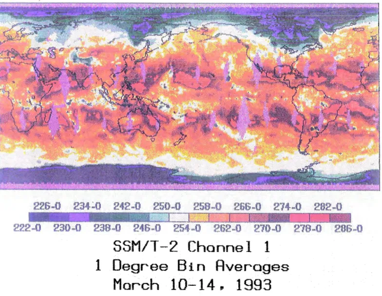
Data were binned into 1 degree latitude X longitude bins and then averaged. Since resolution at nadir is about 50 km, bins twice the size of nadir resolution should be representative for the data.
2.3.1 Channell Brightness Temperature Maps
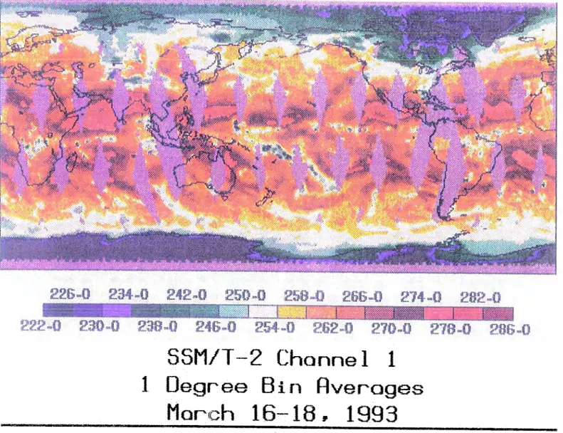
Charmel1, at 183.31 ± 3 GHz, is used for the determination of mid-upper tropospheric water vapor and relative humidity information. As shown below (in Figures 4.1-4.3), the peak of the weighting function for this charmel lies between 3-6 km for the three McClatchey atmospheres. Figures 2.2 and 2.3 are the Channell brightness temperatures for the periods 10-14 March and 16-18 March 1993, respectively.
The areas in red which are located both north and south of the equator (e.g. roughly 20-25° from the equator) delineate the location of subsidence associated with the sub-tropical highs. This prominent feature is also prevalent in the distributions for other frequencies. The subtropical high in the North Atlantic extends from western Africa westward all the way to the Caribbean Sea.
Figure 2.3 suggests a more coherent and stronger ITCZ in the Pacific Ocean (the white and green color shading with several purple pixels). The South Pacific Convergence Zone (SPCZ) (from the central South Pacific extending northwest to east of New Guinea) is also more distinct in this figure. Both features appear cold (and thus moist) in contrast to the the warm (and thus dry) subsiding air poleward of these features.
18
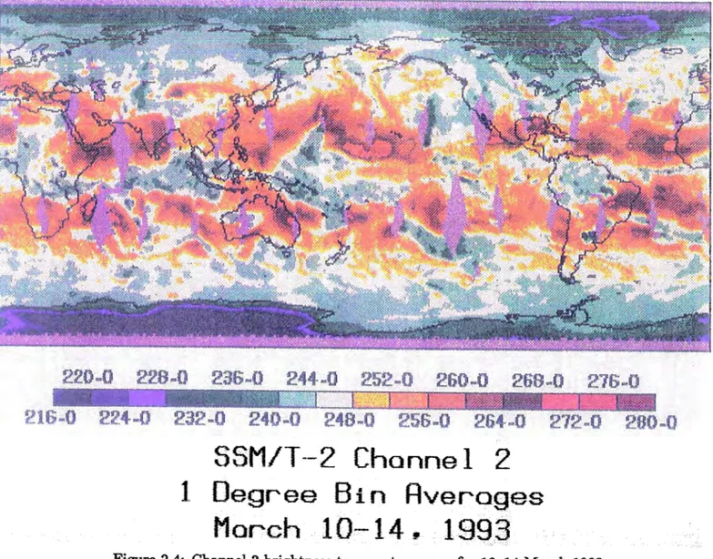
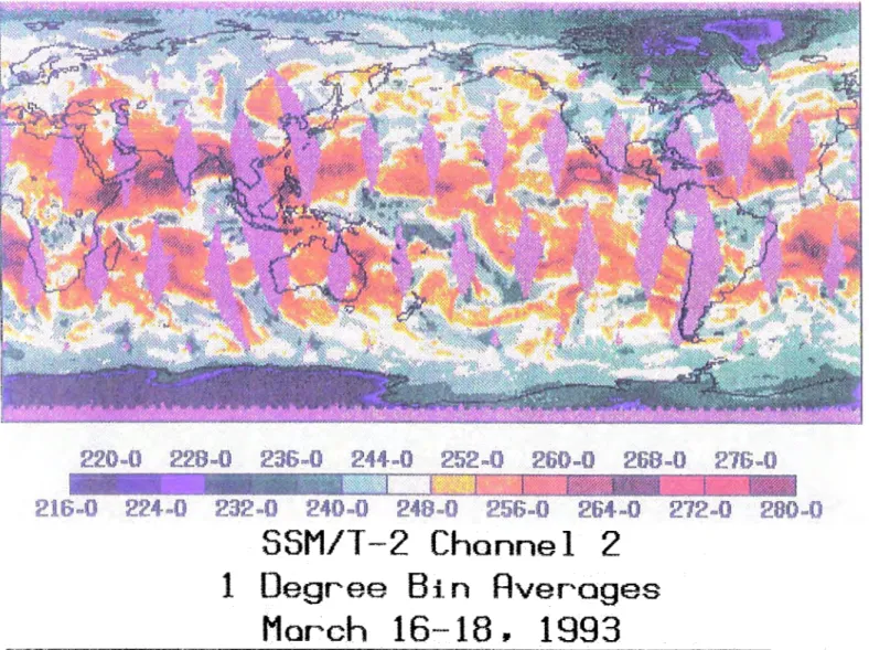
2.3.2 Channel 2 Brightness Temperature Maps
The weighting functions of Channel 2 peak highest in the atmosphere (Figures 4.1-4.3 with peaks between 5-8
km)
and measurements provided by Channel 2 thus applies to upper tropospheric moisture. Figure 2.4 and 2.5 are the Channel 2 brightness temperature maps for the two time periods described above. Maps for this channel have less spread of brightness temperatures than for Channel 1. Channel 2 shows several areas with bigh brightness temperatures over the oceans and these are: (1) in the central North Pacific near 10-15° latitude and near the date line, (2) in the eastern North Pacific south of Baja, California, (3) in the eastern North Atlantic off the west coast of Africa, (4) in the South Atlantic off the coast of Brazil and (5) near Madagascar in the Indian Ocean. These brightness temperatures indicate that the atmosphere is very dry in the upper levels and these regions are also over the subsidence regions indicated in Figures 2.2 and 2.3. The coldest brightness temperatures over the tropical oceans occur near Fiji in the western Pacific and in the central Indian Ocean. The cold brightness temperatures indicate deep convection in these areas and elevated amounts of upper tropospheric moisture.2.3.3 Channel 3 Brightness Temperature Maps
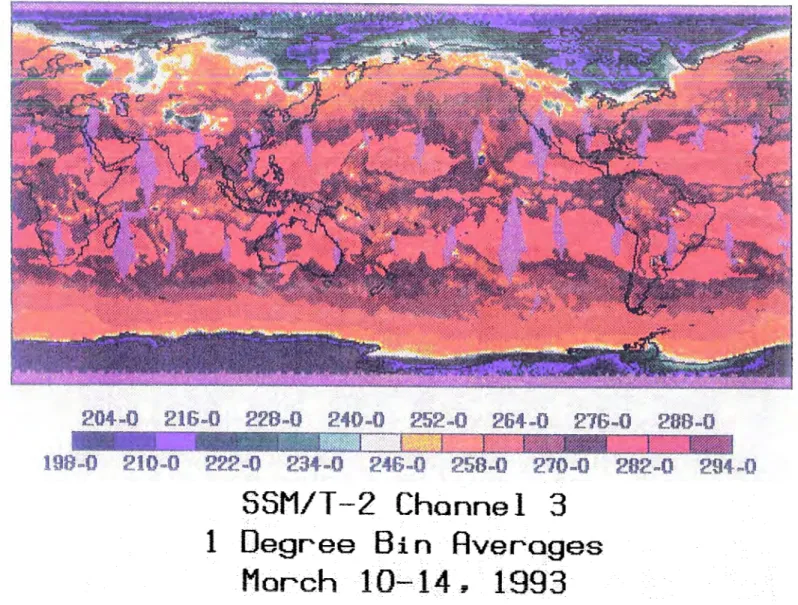
Channel 3, located at 183.31 ± 7 GHz, senses levels of water vapor that occur deeper into the atmosphere according to the location of the weighting function maxima for this channel that are depicted in Chapter 4. Figure 2.6 and 2.7 are the brightness temperature maps for 10-14 March and 16-18 March, respectively. Once again, there exists coherence in the subsidence regions such that the broad areas of red color are the regions of subtropical high pressures underlying those dry regions noted in reference to the maps of Channels 1 and 2 brightness temperature. Similarly, the moist tropical regions where the deepest convection occurs appear relatively cold (indicated by white-green colors).
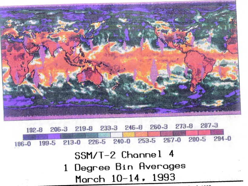
2.3.4 Channel 4 Brightness Temperature Maps
Channel 4, the window channel at 91.655 GHz, primarily senses the surface of the earth. Figures 2.8 and 2.9 are show the brightness temperatures from Channel 4 for the time periods described above. The red color across the land masses (especially Australia)
19
in the southern hemisphere point to clear skies (at least predominantly), a warm surface and a high emissivity for these land masses. This is not surprising when considering that the land has had the entire summer to become warm and dry. The lower emissivity of the adjacent ocean surfaces results in much lower brightness temperatures and it is easy to differentiate between land masses and ocean surfaces.
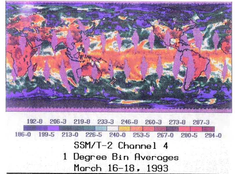
East of Japan there are four curved features with brightness temperatures warmer than the surrounding region. Daily maps of brightness temperatures (not shown) indicate this feature is a mesoscale storm system which has been viewed by the T-2 on successive satellite passes (over several days). The cloud features associated with this low-pressure system show up as warm brightness temperatures over the cold ocean background, resem-bling a comma cloud.
Regions of the tropical oceans show little structure. The yellow and brown colors extend farther south in the Southern Hemisphere as compared to the northern extent in the Northern Hemisphere due to warmer sea surface temperatures and low level moisture over these oceans, since the weighting functions corresponding to this channel peak at /near the surface. Since SSTs typically lag by about two months, SSTs in the southern oceans should be just beginning their fall from the yearly temperature maximum.
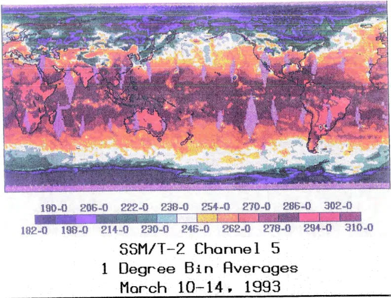
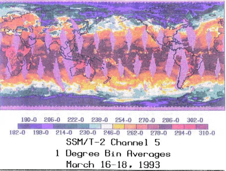
2.3.5 Channel 5 Brightness Temperature Maps
Channel 5, at 150 GHz, is located on the line wing of the absorption line at 183.31 GHz. As shown in Chapter 4, the weighting function for this channel peaks in the lower troposphere or at the earth's surface (depending on the moisture profile of the atmosphere). Figures 2.10 and 2.11 are the brightness temperature maps for the periods 10-14 and 16-18 March 1993. The maps hint at the ITCZ and associated convection (with the light yellow and white pixels) in the tropical oceans. Otherwise, there is not a great deal of structure to the temperature differences that hasn't already been said in the previous subsections.
Figure 2.11 does indicate a stronger SPCZ than does Figure 2.10. Australia has high .brightness temperatures over the entire country likely indicating a high emissivity for the land and a dry atmosphere above it. Again, the land surfaces are easily found in the
20
The brightness temperature maps in Figure 2.2-2.11 provide an opportunity to ex-amine some of the general circulation features of the atmosphere and to see the surface characteristics of ocean and land masses at the frequencies of the SSM/T-2.
2.4 CHANNEL COHERENCE
A helpful way of analyzing and understanding the properties of the T -2 channel bright-ness temperatures is to consider the relationships between channels. Here we consider two regions which are characterized by distinctly different large scale circulation features and thus different temperature and moisture properties.
The two areas selected are located over the Pacific Ocean. The first area corresponds approximately to the TOGA COARE (Coupled Ocean-Atmosphere Response Experiment) domain and is defined as the area 160-170° East longitude and 0-10° South latitude. This area is largely under the control of deep convection and ascent as part of the Hadley and Walker circulations and represents a region of relatively high moisture content at all levels. The brightness temperatures from this area are compared and contrasted with an area in the Eastern Pacific defined by the coordinates 110-120° West longitude and 10-20° North latitude. This East Pacific area is located in a region dominated by a subtropical high with its (assumed) associated strong subsidence and lower column water vapor. Time constraints did not permit a detailed analysis of the cloudiness over these regions during this study.
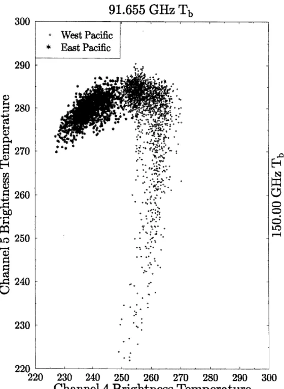
The brightness temperatures for these regions and for the 5 channels are plotted against each other in the form of scatter diagrams. Figure 2.12 shows Channel 5 versus Channel 4 for the two Pacific regions. The East Pacific (EP) region shows a very small scatter for the brightness temperature data. The Channel 4 temperatures are relatively low (as compared to the Channel 5) since this channel is designed to see the sur£~e. As discussed in Chapter 4, the emissivity of the ocean surface is relatively low (,..., 0.7) and it provides a cold background. Channel 5, on the line wing, provides both surface effects and the effects of low level water vapor. The brightness temperature indicates an emission temperature near 280 K. The West Pacific (WP) area shows a window brightness
226-0
234~0242-0 250-0
258 .. 0
266 .. 0
214 .. 0
282-0
-
~_~R"""''''''''--''''' ~ ~!:~~1~r~k~ :.,.,:~-:,~:,
222-0 230;.0
238 .. 0
246-0 254=-0
262 .. 0
210-0 218-0 -286 .. 0
SSM/T-2 Channel 1
1 Degree Bin Averages
March
10-14~
1993
Figure 2.2: Channell brightness temperature ma.p for 10-14 March 1993.
~
226-0
234 ...
Q
242-0
250 .. 0
258-0 266-0
214-0
282-0
. _ ~ _ _
~~t':':c,;-:~--_o_-222 .. 0
230-0
238-0 246-0
254-0 262-0 270 .. 0
278-0
286-0
SSM/T-2 Channel 1
1 Oegree Bin
Averages
Morch 16-18. 1993
Figure 2.3: Channell brightness temperature map for 16-18 March 1993.
M N
~
_ _
f;!~:~~!r:7:,220-0
228-0
236-0
244-0
252 ..
0
260 .. 0
26B~O·.276-0216 .. 0
224 ..
0
232.0 240·0 248;..0
256 .. 0
264;..02"12 ..
0
SSM/T-2 Channel 2
1 Degree Bin Averages
March
10~14.
1993
Figure 2.4: Channel 2 brightness temperature map for 10-14 March 1993.
~ ~
220-0 228-0 236 ... 0
244-0 252.0 260-0 268-0 216-0
I
~--~~'~~;'"
~ ·~k.';:fM!_"'~(l ' , " , "{-/216.0 224.0 232.0 240.0 248-0 256-0 264-0 212-0 280·0
SSM/T-2 Channel 2
1 Degree Bin
Averages
March
16-18.
1993
Figure 2.5: Channel 2 brightness temperature map for 16-18 March 1993.
204~() 216~O
228 .. 0
240-0 252-0264-0 216 .. 0288-0
-
~_~,. :;;'~··i .. ~ ~'''''''''''.'''''f
198..;0210~0
222-0 234-0 246-0 258 .. 0270 .. 0 ·282-0 294 .. 0
SSM/T-2 Channel 3
1 Degree Bin Averages
March
10-14~
1993
Figure 2.6: Channel 3 brightness temperature map for 10-14 March 1993.
~
204 ..
.0
216",.0
228-0 240-0
252-0
264-0 216-0
288 .. 0
. :,;~ ... ~ :':$:~-''''\.~~/ n • • <//. .. ~-. . ~<" ... . ~, .. / "198-0 210 ..
0
222 .. 0
234-.. 0
246-0
258~0210 ..
0
282,.;0
294- .. 0
SSM/T-2
Channel
3
1 Degree Bin
Averages
March
16-18* 1993
Figure 2,7: Cha.n~el 3 brightness temperature map for 16-18 March 1993.
~ m
192-8 206-B
21JJ-B
239-3 246 .. 8
260 .. 3
213 .. 8.
287~a.
-~
_ _
g¥~*\1L',.'::
186;;.0
199-5 213.0
226-5
240-0
253-5
267.0 280 ..
5
294·0
SSM/T-2 Channel 4
1 Degree Bin
Averages
March
10-14, 1993
Figure 2.8: Channel 4 brightness tempera.ture map for 10-14 March 1993.
~
-
t9.2~a..<2Q.f.)-a<·~1{J;.tl~~a-3246
...
82fi() ...
3~73-a
..287 .. fl
186~()
··199-5
213~226-5240-025a~5-267
-0 280 ... 5
294-0
SSM/T-2 Channel 4
1 Degree
Bin Averages
March 16-18, 1993
Figure 2,9: Channel 4 brightness temperature map for 16-18 March 1993.
t-.)
•
186~()
199-5
213~O
226-5
240.()
253-5
267 ..
0280..5 294 .. 0
SSM/T-2 Channel 4
1 Degree Bin
Av~roges
March 16-18. 1993
Figure 2.9: Channel 4 brightness tempera.ture map for 16-18 March 1993.
t-:I 00
190-0 ... 206-0 222-0 238 .. 0
254 ... 0
210-0286-0 302 .. 0
•
~_!Il!IIIIlII\III~hl~: ~ ~r.:t::o\ .. ~~.,182 .. 0
198 .. 0
214 .. 0
230 .. 0
246 ..
0
262~O218-0
294-0
310-0
SSM/T-2 Channel 5
1 Degree Bin Averages
March
10~14,
1993
Figure 2.10: Channel 5 brightness temperatw-e map for 10-14 March 1993.
t-..:)
190 .. 0
206 ..
0
222-0
238 ..
0
254-0 210-0 286-0
302 ..
0
~--- - - 7 -_ _ ~f~~~:g1~;;~ ~. -I182 .. 0
190 .. 0
214 .. 0
230-0
246-0
262-0 278 ... 0
294 ... 0
310-0
SSM/T-2 ChannelS
1 Degree Bin Averages
Morch
16-18~
1993
Figure 2.11: Channel 5 brightness temperature map for 16-18 March 1993.
(..I) <::)
31
temperature of 10-15 degrees higher than the East Pacific area. This likely occurs due to more emission by the water vapor (near the surface, emitting at a high temperature) in the wetter atmosphere in the West Pacific. The scatter of data from the West Pacific indicates that the area contains many inhomogeneities. Possible reasons for this scatter will be discussed later.
Figure 2.13 depicts the brightness temperatures of the 150 GHz channel and the 183
±
7 GHz channel. Since these two channels are adjacent to each other, it is expected that the two channels would be well correlated. For the East Pacific area, the Channel 3 and 5 temperatures are nearly equal, with most of the Channel 3 temperatures within 100 of280 K. For the WP region, Channel 3 becomes opaque more quickly and therefore, most of the temperatures are below 275 K. The vertical correlation of brightness temperature (and therefore water) shows up very well for the WP region. An almost linear relationship between these two channels is inferred by the data.
Figure 2.14 is the scatter plot of the brightness temperatures of Channels 1 and 5. The EP area again exhibits higher brightness temperatures for channels which peak above the surface, implying a dry upper atmosphere. Additionally, there is not much scatter of the data for this region, implying a profile which is nearly invariant. Channel 1 brightness temperatures for the WP region are about 200 colder than the EP region. This indicates
that this channel is sensing water vapor at a colder temperature which means a higher altitude.
Perhaps the best depiction of the differences in the two areas is shown in Figure 2.15. This figure plots the window channel (Channel 4) against the channel closest to the absorption line (Channel 2). Figure 2.15 shows that the EP area has a high Channel 2 brightness temperature, implying the channel peaks well down in the atmosphere. The
WP area has noticeably lower brightness temperatures for Channel 2, indicating a peak of the channel higher in the vertical (and consequently, at a lower thermometric temperature than for the EP). Channe14 brightness temperatures are governed by the low emissivity of the cold ocean surface in the EP and the higher thermal temperature of the surface and lower atmosphere combined for the WP region.
290
230
3291.655 GHz
Tb
() West Pacific
*
East Pacific
. .
.
: 00 0 . _..
.
~. o. o·. .
..
220
~~~~~~~~~--~~~~~~~~220
230
240
250
260
270
280
290
300
Channel 4 Brightness Temperature
33
183.31 ±7
GHz
Tb
<>West Pacific
*
East Pacific
300
1-....
"220
, "200
~~--~~--~--~~--~--~~--~~200
220
240
260
280
300
Channel 3 Brightness Temperature
290
...
~
~ 34183.31 ±:3 GHz
Tb
oWest Pacific
*
East Pacific
~
240
o
'.
..
.
.
230
..
220
~~~~~~~~--~~~~~~~~~220
230
240
250
~!60270
280
290
300
Channell Brightness Temperature
35
183.,31 ±1 GHz
Tb
280
~---~-~~--~~--~~--~-,2"10
Cl) ~ ~~
~~2(>O
S
~
iI.l iI.l Q)E
250
...c:
bO • ..-4 f-4CO
~]
240
~~
0
230
¢West Pacific
*
East Pacific
.'..
.
.
.
..
• o • •"
..."
•
.
"
••
•
... J" ...
•
"
.
..
......
.
...
:.
:..'" • * .. : •"
...
-
.
...
:.
**
...•
220
~~--~~~--~~~~~~~~~~~220
230
240
250
260
270
280
Channel 2 Brightness Temperature
36
Figure 2.16 also shows a distinct difference in the brightness temperatures for the two Pacific areas. This figure depicts the brightness temperatures for Channel 4 versus Channel 1. The explanation of these features is basically the same as the previous paragraph as the Channel 1, mid-upper tropospheric peak for the weighting function, brightness temperature is high for the region with subsidence and is low for the region with an abundance of water vapor. Conversely, the Channel 4 brightness temperatures are high for the TN}l and and relatively low for the EP. SST differences certainly playa part in
these brightness temperature differences, with higher SSTs (which means higher brightness temperatures) for the WP. Additionally, water vapor neat" the surface and cloud effects also contribute to the higher brightness temperatures in the WP region.
The effect of ice and mixed phase and partial cloud cover clouds cannot be quanti-tatively nor qualiquanti-tatively examined from these figures or from the brightness temperature maps. This is an area where future research is needed.
In this section it has been shown that:
1. Areas with distinctly different moisture profiles (such as regions oflarge scale subsi-dence versus moist ascent) can be uniquely identified through the use of brightness temperature plots.
Chapter 3
MICROWAVE RADIATIVE TRANSFER AND WEIGHTING FUNCTIONS
Emission from the atmosphere and the Earth's surface provide the source of radia-tion received at satellite altitude by microwave instruments. Radiaradia-tion detected by these instruments is changed by the processes of absorption, emission and scattering within the atmosphere. These processes depend on the properties of the Earth's surface, atmo-spheric constituents especially water vapor and the concentration of hydrometeors and information about these properties can be retrieved from measurements of this radiation (Stephens, 1993). As stated, detection of atmospheric water vapor, and specifically its vertical profile is the objective of the SSM/T-2 Millimeter Wave Moisture Sounder.
For the frequencies of interest, clear sky absorption arises primarily from water vapor and to a lesser extent oxygen absorption (Waters, 1976.) Ozone also absorbs in this region, but to a much lesser extent than water vapor and oxygen, and ozone absorption has a negligible effect on brightness temperatures. Cloud droplets also absorb in the microwave/millimeter wave region.
Figure 3.1 provides a physical perspective on microwave emission and shows some of the effects of water vapor, surface reflectance, and cloud liquid water on this emission. Case (2) shows the emission spectra found over a cold surface (e.g. ocean) versus case (4) which presents the spectra found over a warm surface (e.g. land). The difference in spectra between case 1 and case 2 shows how water vapor changes the brightness temperatures. These effects lead to temperature decreases over land (warm background land increases over ocean (cold background). Similarly, the change in spectra between cases 2 and 3 show the effects of cloud droplet (Rayleigh) absorption. Finally, the spectra change from cas
39
2 to case 4 is an example of how surface characteristics may change intensities measured by a satellite radiometer.
3.1 TH:E~ RADIATTVE TRANSFER EQUATION FOR MICROWAVE RE-MO'rE SENSING
The radiative transfer equation describes how, in a mathematical sense, radiation is transfen'ed from one layer to another. The generalized fonn of this equation which includes the effects of both absorption and emission of energy is written as:
dI = -k,.,[I - B]ds,
(3.1)
where I is the intensity, kv is the volume absorption coefficient, and B is the emission
represented by Planck's function. Equation
(3.1)
neglects scattering, which is common for many problems in microwave radiative transfer and it also assumes the condition of local thennodynamic equilibrium. The principles of emission-based sensing are used for many atmospheric applications including the remote sensing of sea surface temperature (SST), column water vapor, cloud liquid water content, precipitation rate, temperature profiles, and clouds.3.1.1 Brightness Temperatures
At the wavelength of microwave/millimeter wave radiometers, the Rayleigh-Jeans distribution applies - that is, radiant energy and temperature are synonymous. This temperature is referred to as the brightness temperature, and, for satellite radiometers is a meas1lll'e of the upwelling thenna1 microwave radiation from the medium (in this case the atmosphere) below. Using the Rayleigh-Jeans approximation, assuming specular reflection and for a nadir viewing radiometer, this brightness temperature,
Tb(V),
can be expressed as:Tb(V)
=faoo
exp(-r(h,oo))-y(v,h)T(h)dh+exp(-r(O,oo))
X[(1 _.
R)T6fc
+
R
1
00
I I
300
v
40 DMSP INSTRUMENTS I 2 2 222Nadir Angle
Tsfc=300K
_ - - - -... ~, "r.//-/
, . '\\
..1/
, • /., \ 'f , ' / , 1. '/
\ I
,,"-\' 'I \ / \' 'I \ 1 ",'" \. 1 \I
'" ,. 1 / 11 I 1//
',1
\
I
~ I 1\ /'" I, II I, \, '-,
'". I,
,.I ,;.... \I
: : I f 'I : : \ Vd
,
'
Case
1
Case
2
Case 3
Case
4
180
~~~~~~~~~~~~~~~--,---~o
20
40
60
80 100 120 140 160 180 200
FREQUENCY (GHz)
Figure 3.1: Brightness temperature spectra from 1-200 GHz for cases (1) tropical atmo-sphere with no water vapor and reflectivity (R)
=
0.3; (2) tropical atmosphere (CWV =41.2g/m2) and R
=
0.3; (3) tropical atmosphere with a cloud (LWC=
0.5g/m2) from 1-2Ian and R = 0.3 and case (4) same as case (2) except R = 0.0. The locations of the SSM/I and SSM/T-2 channels are indicated by "r' and "2", respectively.