MODELLING AND FORECASTING INFLATION RATES IN GHANA: AN APPLICATION OF SARIMA MODELS

HÖGSKOLAN DALARNA

SCHOOL OF TECHNOLOGY AND BUSINESS STUDIES

MODELLING AND FORECASTING INFLATION RATES IN GHANA: AN APPLICATION OF SARIMA MODELS

Author:

AIDOO, ERIC

Supervisor

DAO LI

i

HÖGSKOLAN DALARNA

SCHOOL OF TECHNOLOGY AND BUSINESS STUDIES

MODELLING AND FORECASTING INFLATION RATES IN GHANA: AN APPLICATION OF SARIMA MODELS

Author

AIDOO, ERIC

Supervisor

Dao Li

(Master‟s Thesis)

A dissertation submitted to the School of Technology and Business Studies,

Hogskolan Dalarna in partial fulfillment of the requirement for the award of

Master of Science Degree in Applied Statistics.

APRIL, 2010

ii

ACKNOWLEDGEMENT

(Showing gratitude paves way for future assistance)

The completion of this research has been possible through the help of many individuals who supported me in the different stages of this study. I would like to express my deepest appreciation to my supervisor Dao Li. Who despite her heavy schedule has rendered me immeasurable supports by reviewed the manuscript. Her comments and suggestions immensely enriched the content of this work.

I am also grateful to all the lecturers and entire staffs of Dalarna University especially Professor Kenneth Carling, Professor Changli He, Associate Professor Lars Rönnegard, Moudud Alam, Richard Stridbeck and Mikael Moller.

I have also benefited from the help of the many other individuals during my studies at Dalarna University, especially Collins Armah, Amarfio Susana, Fransisca Mensah, Seth Opoku and Emmanuel Atta Boadi.

I extend my sincere gratitude to officials of Ghana Statistical Service Department for their assistance in providing data for this exercise.

Finally, I want to give thanks to the 2010 year group of Masters in Applied Statistics, Hogskolan Dalarna.

iii

DEDICATION

iv

ABSTRACT

Ghana faces a macroeconomic problem of inflation for a long period of time. The problem in somehow slows the economic growth in this country. As we all know, inflation is one of the major economic challenges facing most countries in the world especially those in African including Ghana. Therefore, forecasting inflation rates in Ghana becomes very important for its government to design economic strategies or effective monetary policies to combat any unexpected high inflation in this country. This paper studies seasonal autoregressive integrated moving average model to forecast inflation rates in Ghana. Using monthly inflation data from July 1991 to December 2009, we find that ARIMA (1,1,1)(0,0,1)12 can represent the data behavior of inflation rate in Ghana well. Based on

the selected model, we forecast seven (7) months inflation rates of Ghana outside the sample period (i.e. from January 2010 to July 2010). The observed inflation rate from January to April which was published by Ghana Statistical Service Department fall within the 95% confidence interval obtained from the designed model. The forecasted results show a decreasing pattern and a turning point of Ghana inflation in the month of July.

KEY WORDS: Ghana Inflation, Forecasting, Box-Jenkins Approach, SARIMA model,

v

TABLE OF CONTENTS

LIST OF FIGURES ... vii

1 INTRODUCTION ... 1

2 DATA ... 4

3 METHODOLOGY ... 6

4 MODELLING ... 13

4.1 Model Identification ... 13

4.2 Estimation and Evaluation ... 15

4.3 Forecasting ... 18

5 CONCLUSIONS ... 20

vi

LIST OF TABLES

Table 3.1: Behaviour of ACF and PACF for Non-seasonal ARIMA(p,q) ... 9

Table 3.2: Behaviour of ACF and PACF for Pure Seasonal ARIMA(P,Q)s ... 9

Table 4.1: HEGY Test for Seasonal Unit Root ... 13

Table 4.2: Canova-Hansen Test for Seasonal Unit Root ... 14

Table 4.3: Unit Root Test for Inflation Series in its level form ... 14

Table 4.4: Unit Root Test for First Differenced Inflation Series ... 14

Table 4.5: AIC and BIC for the Suggested SARIMA Models ... 16

Table 4.6: Estimation of Parameters for ARIMA(1,1,1)(0,0,1)12 ... 17

Table 4.7: Estimation of Parameters for ARIMA(1,1,2)(0,0,1)12 ... 17

Table 4.8: ARCH-LM Test for Homoscedasticity ... 17

Table 4.9: Forecast Accuracy Test on Suggested SARIMA Models ... 18

vii

LIST OF FIGURES

Figure 2.1: Monthly Inflation Rates of Ghana (1991:7 - 2009:12) ... 4

Figure 2.2: ACF and PACF of Inflation Rates (1991:7 - 2009:12)... 4

Figure 4.1: ACF and PACF of First Order Differenced Series ... 16

Figure 4.2: Diagnostics Plot of the Residuals of ARIMA(1,1,1)(0,0,1)12 Model ... 17

1

1 INTRODUCTION

NFLATION as we all know is one of the major economic challenges facing most countries in

the world especially African countries with Ghana not being exception. Inflation is a major focus of economic policy worldwide as described by David, F.H. (2001). Inflation causes global concerns because it can distort economic patterns and can result in the redistribution of wealth when not anticipated. Inflation as defined by Webster‟s (2000) is the persistent increase in the level of consumer prices or a persistent decline in the purchasing power of money. Inflation can also be express as a situation where the demand for goods and services exceeds their supply in the economy (Hall, 1982). In real terms, inflation means your money can not buy as much as what it could have bought yesterday. The most common measure of inflation is the consumer price index (CPI) over months, quarterly or yearly. The CPI measures changes in the average price of consumer goods and services. Once the CPI is known, the rate of inflation is the rate of change in the CPI over a period (e.g. month-on-month inflation rate) and usually its units is in percentages. Inflation can be caused by either too few goods offered for sale, or too much money in circulation in the country.

The effect of inflation is highly considered as a crucial issue for a country to face inflation problems. The inflation problems make a lot of people‟s living in a country much harder. People who are living on fixed income suffer most as when prices of commodities rises, these people can not buy as much as they could previously. This situation discourages savings due to the fact that the money is worth more presently than in the future. The exception reduces economic growth because the economy needs a certain level of savings to finance investments which boosts economic growth. Inflation can also discourage investors within and outside the country by reducing their confidence in investments. This is because investors need to be able to expect high possibility of returns in order for them to make financial decisions. Inflation makes it difficult for businesses to plan their operating future. This is due to the fact that it is very difficult to decide how much to produce, because businesses cannot predict the demand for a product in the increasing absolute price. Since people have to charge in order to cover their living costs. Inflation causes uncertainty about the future price, interest rate, and exchange rate, which in turn increases the risks among potential trade partners and discourages the trade between partners.

2 Ghana was the first Sub-Sahara African country to gain political independence from their European colonial rulers –Britain. Ghana has worked hard to deliver on the promise of happiness for its people. Ghana‟s motto, “Freedom and Justice,” demonstrates its many peoples‟ courage and perseverance for freedom, education and socio-political triumph; the results of which can be seen all over the world. All the past governments in Ghana did their best to make a success nation. The economy of Ghana is now considered as one of successful developing countries in Africa and the world as a whole. When discussing the issues of inflation forecasts in Ghana, we found that there has been little research on this study. To develop an effective monetary policy, central banks should possess the information on the economic situation of the country. Such information would enable central banks to predict future macroeconomic developments, see Asel Isakova (2007).

In this study, our main objective is to model and forecast seven (7) months inflation rate of Ghana outside the sample period. The post-sample forecasting is very important for economic policy makers to foresee ahead of time the possible future requirements to design economic strategies and effective monetary policies to combat any expected high inflation rates in the country of Ghana. Forecasts will also play a crucial role in business, industry, government, and institutional planning because many important decisions depend on the anticipated future values of inflation rate. We also believed that this research will serve as a literature for other researchers who wish to embark studies on inflation situation in Ghana.

In order to model the inflation rate, the study starts by analyzing the long behavior of monthly inflation rates of Ghana from July, 1991 to December, 2009 for comprehensive understanding. Following the Box-Jenkins approach, we apply SARIMA models to our time series data in other to model and forecast future monthly inflation rates of Ghana. When it comes to forecasting, there are extensive number of methods and approaches available and their relative success or failure to outperform each other is in general conditional to the problem at hand. The motive for choosing this type of model is based on the behaviour of our time series data. Also in the history of inflation forecasting, this model has proved to perform better as compared to other models.

Box and Jenkins (1976) propose an entire family of models, called AutoRegressive Integrated Moving Average (ARIMA) models. It seems applicable to a wide variety of situations. They have also developed a practical procedure for choosing an appropriate ARIMA model out

3 of this family of ARIMA models. However, selecting an appropriate ARIMA model may not be easy. Many literatures suggest that building a proper ARIMA model is an art that requires good judgment and a lot of experience. ARIMA models are especially suited for short term forecasting. This is because the model places more emphasis on the recent past rather than distant past. This emphasis on the recent past means that long-term forecasts from ARIMA models are less reliable than short-term forecasts, see Pankratz (1983). Seasonal AutoRegressive Integrated Moving Average (SARIMA) model is an extension of the ordinary ARIMA model to analyze time series data which contain seasonal and non-seasonal behaviors. SARIMA model accounts for the seasonal property in the time series. It has been found to be widely applicable in modeling seasonal time series as well as forecasting future values. SARIMA model has also been applied to forecast inflation extensively. The forecasting advantage of SARIMA model compared to other time series models have been investigated by many studies. For example, Aidan et al (1998) used SARIMA model to forecast Irish Inflation, Junttila (2001) applied SARIMA model approach in other to forecast finish inflation, and Pufnik and Kunovac (2006) applied SARIMA model to forecast short term inflation in Croatia. In most of those researches, SARIMA model tends to perform better in terms of forecasting compared to other competent time series models. Schulze and Prinz (2009) applied SARIMA model and Holt-Winters exponential smoothing approach to forecast container transshipment in Germany, according to their results, SARIMA approach yields slightly better values of modeling the container throughput than the exponential smoothing approach.

The structure of the remaining paper is as follows: Section 2 describes the Inflation rate data and macroeconomic background in Ghana. Section 3 introduces the studied SARIMA model in this research. Section 4 analyzes our inflation data and illustrates how the theoretical methodology can be applied for modeling and forecasting. Section 5 presents the concluding remarks which include findings, comments and recommendations.

4

2 DATA

Inflation has been one of the macroeconomic problems bothering Ghana for a long period of time. It has been one of the contributing factors to slow the economic growth in the country.

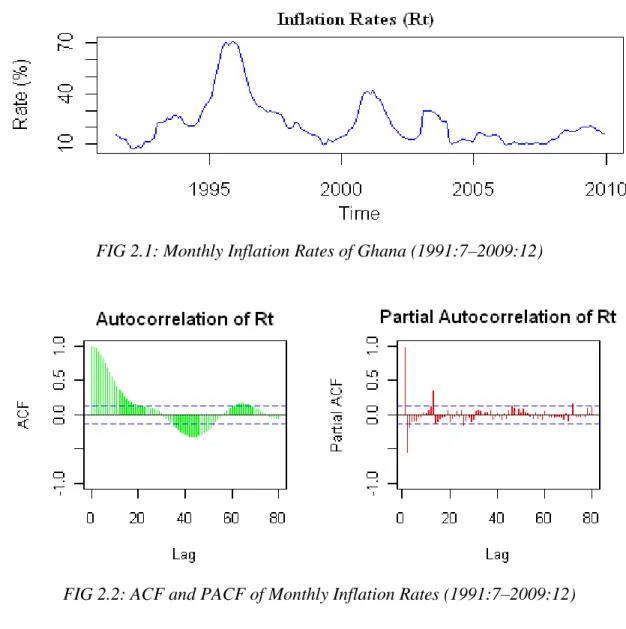
FIG 2.1: Monthly Inflation Rates of Ghana (1991:7–2009:12)

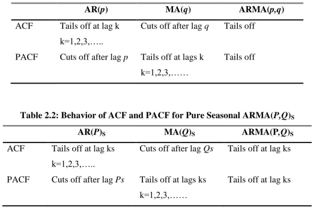
FIG 2.2: ACF and PACF of Monthly Inflation Rates (1991:7–2009:12)

In this research we analyze Two hundred and Twenty Two (222) monthly observations of inflation rate of Ghana from July 1991 to December 2009. The data was obtained from Statistical Service Department of Ghana. The Figure 2.1 and 2.2 above describes the features of the data. The original inflation rate is denoted by Rt.

From Figure 2.1, it can be confirmed that the inflation exhibit volatility starting from somewhere around 1993. The volatility in Ghana inflation series can be attributed to several

5 economic factors. Some of those factors are partly transmitted internationally. Some of those factors that cause inflation in Ghana include increases in monetary aggregates (money supply), exchange rate depreciation, petroleum price increases, and poor agricultural production. For instance, inflation rate increased from 13.30% in December 1992 to 21.50% in January 1993. The rate fluctuated between 21.50% and 26.20% throughout the whole of the year 1993. This increase can be attributed to an increase in petroleum prices. Between the year 1994 and 1995, there was a sharp increase in inflation rate from 22.80% in January 1994 to 70.80% in December 1995. This sharp increase can be attributed to several effects such an increase in petroleum prices in 1993, 1994 and 1995, also the depreciation of the Ghanaian Cedi (¢) at the exchange rate level relative to the same years, a poor performance of agriculture in 1995, and the introduction of a new tax system called VAT1. When the agricultural productivity started improving, between January 1996 and May 1999, inflation rate dropped from 69.20% to 9.40%. From June 1999 to March 2001, the rate of inflation rose again from 10.30% to 41.90%. This sudden rise of inflation could be attributed to an increase world oil prices and a decrease in world market cocoa prices as well as reduction in agricultural performance in the year 2000. From the year 2002 to 2009, the inflation rate fluctuated between 9.50% and 30.0%. Most of these fluctuations were cause by increase in petroleum prices.

In the year 2007, Ghana adopted a monetary police called Inflation Targeting (see Ocran, 2007). Inflation targeting is a money policy in which the central bank target inflation rate and then attempt to direct actual inflation rate towards the target through the use of other monetary policies. There have been a lot of countries in the world who are practicing this policy and this policy has helped others to improve their economy. The target set by the central bank is to bring inflation rate below 10%. Inflation rate was 11% when Ghana adopted this policy. Bringing down inflation represents another challenge. Ghana experienced the rate below 11% through subsequent months until November where it rose to 11.04%. But then as a result of the global food and fuel price increases, it rose and bounded below 21% through the year 2008 and in 2009. From the year 1992 up till now, successive governments have been trying to stabilize inflation within single digit but they have not been successful. Ocran (2007) describe inflation in Ghana as monetary phenomena.

1 _{Value Added Tax: This was a tax which was introduced in 1995 to replace the then sales. But because the value}

6

3

SARIMA - Seasonal AutoRegressive Integrated Moving Average model is an extension of AutoRegressive Integrated Moving Average (ARIMA) model. The ARIMA model is a combination of two univariate time series model which are Autoregressive (AR) model and Moving Average (MA) model. These models are to utilize past information of a time series to forecast future values for the series. The ARIMA model is applied in the case where the series is non-stationary and an initial differencing step (corresponding to the "integrated" part of the model) can make ARMA model applicable to a integrated stationary process. The ARIMA model with its order is presented as ARIMA (p,d,q) model where p, d, and q are integers greater than or equal to zero and refer to the order of the autoregressive, integrated, and moving average parts of the model respectively. The first parameter p refers to the number of autoregressive lags (not counting the unit roots), the second parameter d refers to the order of integration that makes the data stationary, and the third parameter q gives the number of moving average lags. (see Hurvich and Tsai, 1989; Kirchgässner and Wolters, 2007; Kleiber and Zeileis, 2008; Pankratz, 1983; Pfaff, 2008)

A process, {yt} is said to be ARIMA (p,d,q) if t d t d y L y (1 )  is ARMA(p,q). In

general, we will write the model as

(L)(1 L) yt (L)t; {t}~WN(0,2)

d 

 (1)

where t follows a white noise (WN). Here, we define the Lag operator by t t k k

y y

L   and the

autoregressive operator and moving average operator are defined as follows:  L   L L pLp 2 2 1 1 ) ( (2) q qL L L L        2  2 1 1 ) ( (3) 0 ) (L 

 for  1, the process {yt} is stationary if and only if d=0, in which case

it reduces to an ARMA(p,q) process.

The extension of ARIMA model to the SARIMA model comes in when the series contains both seasonal and non-seasonal behavior. This behavior of the series makes the ARIMA model inefficient to be applied to the series. This is because it may not be able to capture the behavior along the seasonal part of the series and therefore mislead to a wrong order selection for

7 non-seasonal component. The SARIMA model is sometimes called the multiplicative seasonal autoregressive integrated moving average denoted by ARIMA(p,d,q)x(P,D,Q)S. This can be

written in is lag form as (Halim & Bisono, 2008): t S t D S d S B B y B B B B   ( )( )(1 ) (1 )  ( )( ) (4) P PB B B B        2  2 1 1 ) ( (5) PS P S S S B B B B       2  2 1 1 ) ( (6) q qB B B B        2  2 1 1 ) ( (7) qS q S S S B B B B       2  2 1 1 ) ( (8) where,

p, d and q are the order of non-seasonal AR, differencing and MA respectively. P, D and Q is the order of seasonal AR, differencing and MA respectively.

yt represent time series data at period t.

_t represent white noise error (random shock) at period t. B represent backward shift operator (Bky_t  y_tk)

S represent seasonal order (s4 for quarterly data and s12 for monthly data).

In the identification stage of model building, we determine the possible models based on the data pattern. But before we can begin to search for the best model for the data, the first condition is to check whether the series is stationary or not. The ARIMA model is appropriate for stationary time series data (i.e. the mean, variance, and autocorrelation are constant through time). If a time series is stationary then the mean of any major subset of the series does not differ significantly from the mean of any other major subset of the series. Also if a data series is stationary then the variance of any major subset of the series will differ from the variance of any other major subset only by chance (see Pankratz, 1983). The stationarity condition ensures that the autoregressive parameters in the estimated model are stable within a certain range as well as the moving average parameters in the model are invertible. If this condition is assured then, the estimated model can be forecasted (see Hamilton, 1994). To check for stationarity, we usually test for the existence or nonexistence of what we called unit root. Unit root test is performed to determine whether a stochastic or a deterministic trend is present in the series. If the roots of the characteristic equation (such as equation 2) lie outside the unit circle, then the series is considered

8 stationary. This is equivalent to say that the coefficients of the estimated model are in absolute value is less than 1 (i.e. i 1 fori 1,,p). There are several statistical tests in testing for

presence of unit root in a series. For series with seasonal and non-seasonal behaviour, the test must be conducted under the seasonal part as well as the non-seasonal part. Some example of the unit root test for the non-seasonal time series are the Fuller and the Augmented Dickey-Fuller (DF, ADF) test, Kwiatkowski-Phillips-Schmidt-Shin (KPSS) test and Zivot-Andrews (ZA) test (see Dickey & Fuller, 1979; Kwiatkowski et al, 1992; Zivot & Andrews, 1992). Also some examples of the unit root test for seasonal time series are Hylleberg-Engle-Granger-Yoo (HEGY)1 test, Canova-Hansen (CH) test etc (see Canova & Hansen,1995; Hylleberg et al,1990; Beaulieu &Miron,1993).

When the series is stationary, the order of the model which is the AR, MA, SAR and SMA terms can be determine. Where AR=p and MA=q represent the non-seasonal autoregressive and moving average parts respectively and SAR=P and SMA=Q represent the seasonal autoregressive and moving average parts respectively as described earlier. To determine these orders, we use the sample autocorrelation function (ACF)2 and partial autocorrelation function (PACF) of the stationary series. The ACF and PACF give more information about the behavior of the time series. The ACF gives information about the internal correlation between observations in a time series at different distances apart, usually expressed as a function of the time lag between observations. These two plots suggest the model we should build. Checking the ACF and PACF plots, we should both look at the seasonal and non-seasonal lags. Usually the ACF and the PACF has spikes at lag k and cuts off after lag k at the non-seasonal level. Also the ACF and the PACF has spikes at lag ks and cuts off after lag ks at the seasonal level. The number of significant spikes suggests the order of the model. The Table 3.1 and 3.2 below describes the behaviour of the ACF and PACF for both seasonal and the non-seasonal series (see Shumway and Stoffer, 2006)

1 _{The HEGY test was first applied by the authors to test for seasonal unit root in quarterly data. The test was later}

extended by some to authors such as Beaulieu & Miron, to test for seasonal unit root in monthly data. The CH test also use similar procedure but in different format.

2

The ACF and PACF are plot that display the estimated autocorrelation and partial autocorrelation coefficients after fitting autoregressive models of successively higher orders to the time series.

9

Table 3.1: Behavior of ACF and PACF for Non-seasonal ARMA(p,q)

AR(p) MA(q) ARMA(p,q)

ACF Tails off at lag k k=1,2,3,…..

Cuts off after lag q Tails off

PACF Cuts off after lag p Tails off at lags k k=1,2,3,……

Tails off

Table 2.2: Behavior of ACF and PACF for Pure Seasonal ARMA(P,Q)S

AR(P)S MA(Q)S ARMA(P,Q)S

ACF Tails off at lag ks k=1,2,3,…..

Cuts off after lag Qs Tails off at lag ks

PACF Cuts off after lag Ps Tails off at lags ks k=1,2,3,……

Tails off at lag ks

Though the ACF and PACF assist in determine the order of the model but this is just a suggestion on where the model can be build from. It becomes necessary to build the model around the suggested order. In this case several models with different order can be considered. The final model can be selected using a penalty function statistics such as Akaike Information

Criterion (AIC or AICc) or Bayesian Information Criterion (BIC). See Sakamoto et. al. (1986);

Akaike (1974) and Schwarz (1978). The AIC, AICc and BIC are a measure of the goodness of fit of an estimated statistical model. Given a data set, several competing models may be ranked according to their AIC, AICc or BIC with the one having the lowest information criterion value being the best. These information criterion judges a model by how close its fitted values tend to be to the true values, in terms of a certain expected value. The criterion value assigned to a model is only meant to rank competing models1 and tell you which the best among the given alternatives is. The criterion attempts to find the model that best explains the data with a

1 _{If two or more different models have the same or similar AIC or BIC values then the principles of parsimony can}

also be applied in order to select a good model. This principle states that a model with fewer parameters is usually better as compared to a complex model. Also some forecast accuracy test between the competing models can also help in making a decision on which model is the best.

10 minimum of free parameters but also includes a penalty that is an increasing function of the number of estimated parameters.

This penalty discourages over fitting. In the general case, the AIC, AICc and BIC take the form as shown below:          n RSS n k or L k

AIC 2 2log( ) 2 log (9)

1 ) 1 ( 2      k n k k AIC AICc (10) ) log( ) log( ) log( ) log( 2 2 n n k or n k L BIC   _e  (11) where

k: is the number of parameters in the statistical model, (p+q+P+Q+1)

L: is the maximized value of the likelihood function for the estimated model.

RSS: is the residual sum of squares of the estimated model.

n : is the number of observation, or equivalently, the sample size

2 e

 : is the error variance

The AICc is a modification of the AIC by Hurvich and Tsai (1989) and it is AIC with a second order correction for small sample sizes. Burnham & Anderson (1998) insist that since AICc converges to AIC as n gets large, AICc should be employed regardless of the sample size.

The next step in ARIMA model building after the Identification of the model is to estimate the parameters of the chosen model. The method of maximum likelihood estimation (MLE) and other methods can be used in this section. At this stage we get precise estimates of the coefficients of the model chosen at the identification stage. That is we fit the chosen model to our time series data to get estimates of the coefficients. This stage provides some warning signals about the adequacy of our model. In particular, if the estimated coefficients do not satisfy certain mathematical inequality conditions1, that model is rejected. Example it is believed that for a chosen model to satisfy ARIMA conditions, the absolute value of the estimated parameters must be always less than unity.

1 _{After the estimation of the parameters of the model, usually the assumptions based on the residuals of the fitted}

model are critically checked. The residuals are the difference between the observed value or the original observation and the estimate produced by the model. For the case of ARIMA model the assumption or the condition is that the residuals must follow a white noise process. If this assumption is not met, then necessary action must be taking.

11 After estimating the parameters of ARIMA model, the next step in the Box-Jenkins approach is to check the adequacy of that model which is usually called model diagnostics. Ideally, a model should extract all systematic information from the data. The part of the data unexplained by the model (i.e., the residuals) should be small. The diagnostic check is used to determine the adequacy of the chosen model. These checks are usually based on the residuals of the model. One assumption of the ARIMA model is that, the residuals of the model should be white noise. A series {_t} is said to be white noise if {_t}is a sequence of independent and identically distributed random variable with finite mean and variance. In addition if {t}is

normally distributed with mean zero and variance2, then the series is called Gaussian White Noise. For a white noise series the, all the ACF are zero. In practice if the residuals of the model is white noise, then the ACF of the residuals are approximately zero. If the assumption of are not fulfilled then different model for the series must be search for. A statistical tool such as Ljung-Box Q statistic can be used to determine whether the series is independent or not. Statistical tool such as ARCH–LM test and Shapiro normality test can also be used to check for homoscedasticity and normality among the residuals respectively.

The last step in Box-Jenkins model building approach is Forecasting1. After a model has passed the entire diagnostic test, it becomes adequate for forecasting. Forecasting is the process of making statements about events whose actual outcomes have not yet been observed. It is an important application of time series. If a suitable model for the data generation process (DGP) of a given time series has been found, it can be used for forecasting the future development of the variable under consideration. In ARIMA models as described by several researchers have proved to perform well in terms of forecasting as compare to other complex models. Using

For example given ARIMA (0,1,1)(1,0,1)12 we can forecast the next step which is given by (see

Cryer & Kung-Sik, 2008)

13 12 1 13 12 1 (   )             t t t t t t t t y y y y      (12) 13 12 1 13 12 1               t t t t t t t t y y y y      (13)

1 _{Forecasting results from ARIMA models in general are better as compare to other linear time series models. But the}

problem with the ARIMA models in terms of forecasting is that, since the model lack long memory properties it cannot be used to forecast for long period.

12 The one step ahead forecast from the origin t is given by

12 11 12 11 1       t  t  t  t  t   t t y y y y      (14)

The next step is

11 10 11 10 1 2        t  t  t  t   t t y y y y      (15)

and so forth. The noise terms 13,12,11,10,,1(as residuals) will enter into the forecasts for lead times l 1,2,3,,13but for l13 the autoregressive part of the model takes over and we have 13 13 12 1    _{  }  y y y forl yt l t l t l t l   (16)

To choose a final model for forecasting the accuracy of the model must be higher than that of all the competing models. The accuracy for each model can be checked to determine how the model performed in terms of in-sample forecast. Usually in time series forecasting, some of the observations are left out during model building in other to access models in terms of out of sample forecasting also. The accuracy of the models can be compared using some statistic such as mean error (ME), root mean square error. (RMSE), mean absolute error (MAE), mean percentage error (MPE), mean absolute percentage error (MAPE) etc. A model with a minimum of these statistics is considered to be the best for forecasting.

13

4 MODELLING

4.1 Model Identification

Looking at the sample ACF and PACF plot of the series in Figure 2.2, there is non-seasonal and seasonal pattern in the series. To confirm the proper order of differencing filter, we can perform both seasonal and non-seasonal unit root test. Using CH and HEGY test, we can test seasonal unit root in the series. Seasonal frequencies in monthly data are

6 6 5 , 3 , 3 2 , 2 ,    

 and . These are

equivalent to 6, 3, 4, 2, 5 and 1 cycles per year respectively (Hylleberg et. al,1990; Canova and Hansen, 1995). The null hypothesis to be tested in HEGY test is, „there exist seasonal unit root‟. Also the null hypothesis to be tested in CH test is „there exist stationarity at all seasonal cycles‟. Table 4.1 and 4.2 present the results on our data from the HEGY and CH test respectively. From the HEGY test results, we reject the null hypothesis of unit root at the seasonal frequency and fail to reject the presence of unit root at the non-seasonal frequency at 5% level. Also from the CH test results, we fail to reject the null hypothesis of stationarity at all seasonal cycles at 5% level. This means that the seasonal cycles at all the frequencies are deterministic or that the contribution from these frequency components is small. Thus, at seasonal level, we do not need to make differences for data.

Table 4.1: HEGY Test for Seasonal Unit Root

Note: * seasonal unit root null hypothesis is rejected at 5% significant

Auxiliary Regression Seasonal Frequency Constant Constant +Trend

0 : 1  test  t 0 -2.123 -3.164 0 : ₂  test  t  -6.667* -6.655* 0 : 3  4  test   F  2 47.072* 47.016* 0 : 5  6  test   F 2 3 42.240* 42.453* 0 : 7  8  test   F  3 46.989* 47.093* 0 : 9  10  test   F 5 6 38.322* 37.677* 0 : ₁₁  ₁₂  test   F  6 36.753* 36.122*

14

Table 4.2: Canova -Hansen Test for Seasonal Unit Root

Frequency L -statistic Critical value

6 6 5 , 3 , 3 2 , 2 ,      and _{0.615* 2.75}

Note: * fail to reject null hypothesis of stationary at 5% significant

Also using KPSS test, we test the null hypothesis that the original series is stationary at the non-seasonal level. From the test results as shown in Table 4.3, since the calculated value is inside the critical region at 5% level, we reject the null hypothesis that the series is stationary. Both ADF and ZA test also confirms the existence of unit root under the situation where either a constant or constant with linear trend were included in the tests. Since the series is stationary at the non-seasonal level, it makes it necessary for first non-non-seasonal differencing of the series to render it stationary. Considering the first non-seasonal differenced series, we use KPSS test the null hypothesis that the first non-seasonal differenced series is stationary. From the test results as shown in Table 4.4; since the calculated value is outside the critical region at 5% level of significance, we fail to reject the null hypothesis that the first differenced series is stationary. Also both ADF and ZA test also confirms the non-existence of unit root under the situation where either a constant or both constant and linear trend were included in the test. Therefore, the difference order should be at least one at non-seasonal level.

Table 4.3: Unit Root Test for Inflation Series in its level form

Test type

Constant Constant + Trend

Critical Value Test statistic Critical Value Test statistic

ADF -2.88 -2.303 -3.43 -2.633

KPSS 0.463 0.897 0.146 0.223

ZA -4.80 -2.213 -5.08 -4.5456

Table 4.4: Unit Root Test for First Differenced Inflation series

Test type

Constant Constant + Trend

Critical Value Test statistic Critical Value Test statistic

ADF -2.88 -5.875 -3.43 -5.882

KPSS 0.463 0.079 0.146 0.060

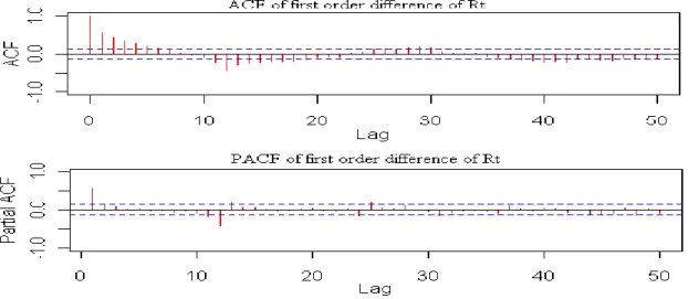
15 The next step in the model building procedure is to determine the order of the AR and MA for both seasonal and non-seasonal components. This can be suggested by the sample ACF and PACF plots based on the Box-Jenkins approach. From Figure 4.1, ACF tails of at lag 2 and the PACF spike at lag 1, suggesting that q2 and p1 would be need to describe these data as coming from a non-seasonal moving average and autoregressive process respectively. Also looking at the seasonal lags, both ACF and PACF spikes at seasonal lag 12 and drop to zero for other seasonal lags suggesting that Q1 and P1 would be need to describe these data as coming from a seasonal moving average and autoregressive process. Hence ARIMA (1,1,2)(1,0,1)12 could be a possible model for the series.

FIGURE 4.1: ACF/PACF of First Order Difference Series

4.2 Model Estimation and Evaluation

After the model has been identified, we use conditional-sum-of-squares to find starting values of parameters, then do the maximum likelihood estimate for the proposed models. The procedure for choosing these models relies on choosing the model with the minimum AIC, AICc and BIC. The models are presented in Table 4.5 below with their corresponding values of AIC, AICc and BIC. Among those possible models, comparing their AIC, AICc and BIC as shown in Table 4.5, ARIMA (1,1,1)(0,0,1)12 and ARIMA (1,1,2)(0,0,1)12 were chosen as the appropriate model that

16

Table 4.5: AIC and BIC for the Suggested SARIMA Models

Model AIC AICc BIC

ARIMA(1,1,1)(0,0,1)12 816.27 816.46 829.87

ARIMA(1,1,2)(0,0,1) 12 816.35 816.63 833.34

ARIMA(1,1,1)(1,0,1) 12 817.20 817.48 834.19

ARIMA(1,1,2)(1,0,1) 12 817.55 817.95 837.94

ARIMA(1,1,0)(0,0,1) 12 823.65 823.76 833.85

From our derived models, using the method maximum likelihood the estimated parameters of the models with their corresponding standard error is shown in the Table 4.6 and 4.7 below. Based on 95% confidence level we conclude that all the coefficients of the ARIMA(1,1,1)(0,0,1)12 model are significantly different from zero and the estimated values

satisfy the stability condition. On the other hand based on the 95% confidence level it can be seen that the MA(2) parameter for ARIMA(1,1,2)(0,0,1)12 model is not significant. Hence after

removing the MA(2) term from the model, it then reduce to ARIMA(1,1,1)(0,0,1)12 model.

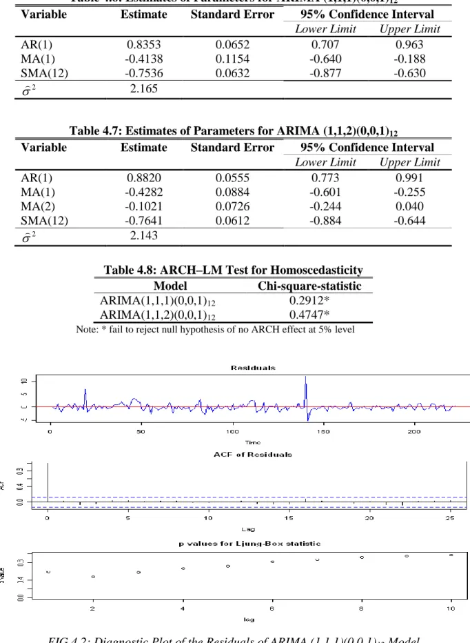
In time series modeling, the selection of a best model fit to the data is directly related to whether residual analysis is performed well. One of the assumptions of ARIMA model is that, for a good model, the residuals must follow a white noise process. That is, the residuals have zero mean, constant variance and also uncorrelated. From Figure 4.3 below, the standardized residual reveals that the residuals of the model have zero mean and constant variance. Also the ACF of the residuals depicts that the autocorrelation of the residuals are all zero, that is to say they are uncorrelated. Finally, the p-values for the Ljung-Box statistic in the third panel all clearly exceed 5% for all lag orders, indicating that there is no significant departure from white noise for the residuals. To support the information displayed by Figure 4.3, we use the ARCH–LM and t test to test for constant variance and zero mean assumption respectively. From the ARCH–LM test results as shown in Table 4.8, we fail to reject the null hypothesis of no ARCH effect (homoscedasticity) in the residuals of the selected model. Also from t test results, since the p-value of 0.871 is greater than 5% alpha level, we fail to reject the null hypothesis that, the mean of the residuals is approximately equal to zero. Hence, we conclude that there is a constant variance among residuals of the selected model and the true mean of the residuals is approximately equal to zero. Thus, the selected model satisfies all the model assumptions. Since our model ARIMA (1,1,1)(0,0,1)12 satisfies all the necessary assumptions, now we can say that

17

Table 4.6: Estimates of Parameters for ARIMA (1,1,1)(0,0,1)12

Variable Estimate Standard Error 95% Confidence Interval

Lower Limit Upper Limit

AR(1) 0.8353 0.0652 0.707 0.963

MA(1) -0.4138 0.1154 -0.640 -0.188

SMA(12) -0.7536 0.0632 -0.877 -0.630

2

 2.165

Table 4.7: Estimates of Parameters for ARIMA (1,1,2)(0,0,1)12

Variable Estimate Standard Error 95% Confidence Interval

Lower Limit Upper Limit

AR(1) 0.8820 0.0555 0.773 0.991 MA(1) -0.4282 0.0884 -0.601 -0.255 MA(2) -0.1021 0.0726 -0.244 0.040 SMA(12) -0.7641 0.0612 -0.884 -0.644 2  2.143

Table 4.8: ARCH–LM Test for Homoscedasticity Model Chi-square-statistic

ARIMA(1,1,1)(0,0,1)12 0.2912*

ARIMA(1,1,2)(0,0,1)12 0.4747*

Note: * fail to reject null hypothesis of no ARCH effect at 5% level

18

4.3 Forecasting

Forecasting plays an important role in decision making process. It is a planning tool which helps decision makers to foresee the future uncertainty based on the behavior of past and current observations. Forecasting as describe by Box and Jenkins (1976), provide basis for economic and business planning, inventory and production control and control and optimization of industrial processes. Forecasting is the process of predicting some unknown quantities. From previous studies, most research work has found that the selected model is not necessary the model that provides best forecasting. In this sense further forecasting accuracy test such as ME, RMSE, MAE etc. must be performed on the two obtained. Table 4.9 present the accuracy test for both models. From the results, it can be seen that, most of the accuracy test favor ARIMA (1,1,2)(0,0,1)12 model which has higher information criterion. But comparing the results

critically, the figures for both model seems almost the same. Using Diebold-Mariano test, we can test, we can compare the predictive accuracy from both model. From the results, since the p-value of 0.5648 is greater than alpha value of 0.05, we fail to reject the null hypothesis that two model have the same accuracy forecast. Hence we use the model for which we have estimated its parameters.

Once our model has been found and its parameters have been estimated, we then use it to make our prediction. The Table 4.10 below summarizes the forecasting results of the inflation rates over the period January 2010 to July 2010 with 95% confidence interval.

Comparing the predicted rate for January with the observed rate, we can see that the predicted value is close to the true value which were observed and published by the Ghana Statistical Service Department. Also, all of the observed values fall inside the confidence interval. Hence, we can say that, ARIMA (1,1,1)(0,0,1)12 model is adequate to be used to forecast monthly

inflation rate in Ghana.

Table 4.9: Forecast Accuracy Test on the Suggested SARIMA Models

Model ME RMSE MAE MPE MAPE MASE

ARIMA(1,1,1)(0,0,1)12 -0.008 1.468 0.941 -0.278 4.628 0.679

19

Table 4.10: ARIMA(1,1,1)(0,0,1)12 Forecasting Results for Monthly Inflation Rates

Month Forecast (%) Observe Value (%) Lower Bound Upper Bound

January 14.57 14.78 11.68 17.45 February 14.63 14.23 9.62 19.64 March 14.32 13.32 7.16 21.48 April 13.46 11.66 4.14 22.78 May 12.58 1.12 24.04 June 11.30 -2.26 24.87 July 11.68 -3.95 27.31

The Figure 4.4 below display the original inflation and the fitted values produced by the obtained ARIMA(1,1,1)(0,0,1)12 model. It can be confirm that the model somehow fit the data

better. The figure also displays how the forecasted values behave.

From the forecasting results, because the process is non-stationary, the confidence interval becomes wider as the number of forecast increase. Thus, the large forecast interval suggests a very high stochasticity in the data.

20

5 CONCLUSION

Following the Box-Jenkins approach, Seasonal Autoregressive Integrated Moving Average (SARIMA) was employed to analyse monthly inflation rate of Ghana from July 1991 to December 2009. The study mainly intended to forecast the monthly inflation rate for the coming period of January, 2010 to July 2010.

Based on minimum AIC, AICc and BIC value, the best-fitted SARIMA models tends to be ARIMA(1,1,1)(0,0,1)12 and ARIMA(1,1,2)(0,0,1)12 model. After the estimation of the

parameters of selected model, a series of diagnostic and forecast accuracy test were performed. Having satisfied all the model assumptions, ARIMA(1,1,1)(0,0,1)12 model was judge to be the

best model for forecasting.

The forecasting results in general revealed a decreasing pattern of inflation rate over the forecasted period and turning point at the month of July. In light of the forecasted results, policy makers should gain insight into more appropriate economic and monetary policy in other to combat such increase in inflation rate which is yet to occur at the month of July.

The accuracy of forecasted future values is the core point for every forecaster. This is because the forecasted values will affect the quality of the policies implemented based on this forecast. With this motive, it is therefore recommend that future research on this topic is of great concerned and it will be helpful to access the performance of the model used in this research in terms of forecast precision as compare to other time series models. The precision of forecast does not based on complexity or simplicity of the model used.

From the description of the Ghana inflation rates behavior, it was found that, an increase in world oil prices always leads to increase in Ghana inflation rate. In the next few years Ghana will be an oil producer and it is believe that if the county managed the newly found natural resources (oil) well, then increase in world market oil price will not affect inflation in the country so much. This will also pave way for policy makers to study inflation situation in Ghana in other to determine other factors that contribute to high inflation rates in the country.

21

REFERNCES

[1] Adam, C., Ndulu, B. and Sowa, N.K (1996). Liberalization and Seigniorage Revenue in Kenya, Ghana and Tanzania. The Journal of Development Studies, 32(4, April), 531–53. [2] Aidan, M., Geoff, K. and Terry, Q. (1998). Forecasting Irish Inflation Using ARIMA

Models. CBI Technical Papers 3/RT/98:1-48, Central Bank and Financial Services Authority of Ireland.

[3] Akaike, H.(1974). A New Look at the Statistical Model Identification. IEEE Transactions

on Automatic Controll 19 (6): 716–723.

[4] Amediku, S. (2006). Stress Test of the Ghanaian Banking Sector: A VAR Approach. BOG

Working Papers 2006/02, Bank of Ghana.

[5] Asel, I. (2007). Modeling and Forecasting Inflation in Developing Countries: The Case of Economies in Central Asia. CERGE-EI Discussion Papers 2007-174, Center for Economic Research and Graduate Education, Academy of Science of the Czech Republic Economic Institute.

[6] Beaulieu, J. & Miron, J. (1993), Seasonal unit roots in aggregate U.S. data. Journal of

Econometrics, 54: 305-328.

[7] Box, G.E.P. & Jenkins, G.M. (1976) Time Series Analysis: Forecasting and Control. Holden-Day, San Francisco.

[8] Brockwell, P. J. & Davis, R. A. (1996) Introduction to Time Series and Forecasting. Springer, New York.

[9] Burnham, K.P., & Anderson, D.R. (1998). Model Selection and Inference. Springer-Verlag, New York.

[10] Buss, G. (2009). Comparing forecasts of Latvia's GDP using Simple Seasonal ARIMA models and Direct versus Indirect. MPRA Paper No. 16825, Munich Personal RePec Archive.

[11] Canova, F & Hansen, B.E (1995), Are Seasonal Patterns Constant Over Time? A Test for Seasonal Stability. Journal of Business and Economic Statistics, 13, 237-252.

[12] Chan, N.H (2002) Time Series Application To Finance. John Wiley & Sons, Inc., USA. [13] Cowpertwait, P.S.P & Metcalfe, A.V. (2009) Introductory Time Series with R. Springer

22 [14] Cromwell, J.B., LABYS, W.C., & Terraza M. (1994) Univariate Tests for Time Series Models. Sage University Paper series on Quantitative Applications in the Social Sciences, 07-099. Thousand Oaks, CA: Sage.

[15] Cryer J.D & Kung-Sik C. (2008) Time Series Analysis with Applications in R. 2Ed. Springer Science +Business Media, LLC, NY, USA.

[16] David, F.H. (2001) Modelling UK Inflation, 1875-1991. Journal of Applied Econometrics, 16(3): 255-275.

[17] De Brouwer, G. & Neil, R.E. (1998). Modelling Inflation in Australia. Journal of Business

& Economic Statistics, American Statistical Association, 16(4): 433-49.

[18] Dickey, D.A. & Fuller, W.A. (1979). Distribution of the Estimators for Autoregressive Time Series with Unit Root. Journal of the American Statistical Association, 74: 427-431.

[19] Dickey, D.A. & Fuller, W.A. (1981). Likelihood Ratio Statistics for Autoregressive Time Series with a Unit Root. Econometrica, 49(4), 1057-1072.

[20] Diebold, F.X. and Mariano, R.S. (1995) Comparing Predictive Accuracy. Journal of

Business and Economic Statistics, 13, 253-263.

[21] Engle, R.F (2001). GARCH 101: The Use of ARCH/GARCH Models in Applied Econometrics", Journal of Economic Perspectives, 15(4): 157-168

[22] Fedderke, J.W. & Schaling, E. (2005). Modelling Inflation in South Africa: A Multivariate Cointegration Analysis. South African Journal of Economics, 73(1): 79-92.

[23] Franses, P.H. (1990), Testing for Seasonal Unit Roots in Monthly Data, Technical Report 9032, Econometric Institute.

[24] Halim, S. & Bisono, I.N. (2008). Automatic Seasonal Autoregressive Moving Average Models and Unit Root Test Detection. International Journal of Management Science and

Engineering Management, 3(4): 266-274

[25] Hall, R. (1982). Inflation, Causes and Effects. University of Chicago Press, Chicago.

[26] Hamilton, J. D. (1994). Time Series Analysis. Princeton Univ. Press, Princeton New Jersey. [27] Hellerstein, R. (1997). “The Impact of Inflation” Regional Review, Winter 1997, 7(1). [28] Hurvich, C.M., & Tsai, C.L (1989). Regression and Time Series Model Selection in Small

Sample. Biometrika, 76: 297-307.

[29] Hylleberg, S., Engle, R., Granger, C. & Yoo, B. (1990), Seasonal Integration and Cointegration. Journal of Econometrics, 44: 215-238.

23 [30] Kenji, M. & Abdul N. (2009). Forecasting Inflation in Sudan. IMF Working Papers 09/132,

International Monetary Fund.

[31] Kihoro, J.M., Otieno, R.O., & Wafula, C. (2004). Seasonal Time Series Forecasting: A Comparactive Study of ARIMA and ANN Models. African Journal of Science and

Technology, 5(2): 41-49

[32] Kirchgässner, G &Wolters, J. (2007) Introduction To Modern Time Series Analysis. Springer-Verlag Berlin Heidelberg

[33] Kivilcim, M. (1998). The Relationship between Inflation and the Budget Deficit in Turkey.

Journal of Business and Economic Statistics, 16(4): 412-422.

[34] Kleiber, C. & Zeileis, A. (2008) Applied Econometrics with R. Springer Science +Business Media, LLC, NY, USA.

[35] Kwiatkowski, D., Phillips, P. C. B., Schmidt, P. & Shin, Y. (1992): Testing the Null Hypothesis of Stationarity against the Alternative of a Unit Root. Journal of Econometrics 54, 159–178.

[36] Junttila, J. (2001). Structural breaks, ARIMA Model and Finnish Inflation Forecasts

International Journal of Forecasting, 17: 203–230

[37] Mame, A.D. (2007). Modeling Inflation for Mali. IMF Working Papers 07/295, International Monetary Fund.

[38] Ocran, M.K. (2007). A Modelling of Ghana's Inflation Experience: 1960–2003. African

Economic Research Consortium, RP_169.

[39] Michael, H.C. (1981).U.S. inflation and the import demand of Ghana and Nigeria, 1967– 1976. Journal of The Review of Black Political Economy, 11(2), 217-228.

[40] Pankratz, A. (1983) Forecasting with Univariate Box-Jenkins Models: Concepts and Cases. John Wily & Sons. Inc. USA

[41] Pfaff, B. (2008) Analysis of Integrated and Cointegrated Time Series with R. 2Ed, Springer Science +Business Media, LLC, NY, USA.

[42] Phillips, P.C.B. and Perron, P. (1988), Testing for a unit root in time series regression, Biometrika, 75(2), 335–346.

[43] Pufnik, A. and Kunovac, D. (2006). Short-Term Forecasting of Inflation in Croatia with Seasonal ARIMA Processes. Working Paper, W-16, Croatia National Bank.

24 [44] R Development Core Team (2009). R: A Language and Environment for Statistical Computing. R Foundation for Statistical Computing, Vienna, Austria. ISBN 3-900051-07-0, URL http://www.R-project.org.

[45] Sakamoto, Y., Ishiguro, M., and Kitagawa G. (1986). Akaike Information Criterion Statistics. D. Reidel Publishing Company.

[46] Schulz, P.M. and Prinz, A. (2009). Forecasting Container Transshipment in Germany. Applied Economics, 41(22): 2809-2815

[47] Schwarz, G. E. (1978). Estimating the Dimension of a Model. Annals of Statistics 6 (2): 461–464.

[48] Shumway, R.H. and Stoffer, D.S. (2006)Time Series Analysis and Its Applications With R Examples 2Ed, Springer Science +Business Media, LLC, NY, USA.

[49] Sowa, N.K. (1996). Policy Consistency and Inflation in Ghana. African Economic Research

Consortium, RP_43.

[50] Sowa, N.K. and Kwakye, J. (1991). Inflationary Trends and Control in Ghana. African

Economic Research Consortium, RP_22.

[51] Tim, C. and Dongkoo, C. (1999). Modelling and Forecasting Inflation in India. IMF Working Papers 99/119, International Monetary Fund

[52] Tsay, R.S. (2002) Analysis of Financial Time Series. John Wiley & Sons, Inc. USA

[53] Webster, D. (2000). Webster's New Universal Unabridged Dictionary. Barnes & Noble Books, New York

[54] Zivot, E. and Andrews, D. W.K. (1992), Further Evidence on the Great Crash, the Oil-Price Shock, and the Unit-Root Hypothesis, Journal of Business & Economic Statistics, 10(3), 251–270.