Fertility and Earnings in Sweden

(1)

Fertility and Earnings in Sweden

A study of first births and couples’ earnings in Sweden

MASTER THESIS WITHIN: Economics NUMBER OF CREDITS: 30 ECTS PROGRAMME OF STUDY: Civilekonom AUTHOR: Wilma Bolkéus

(2)

Acknowledgements

I would like to thank my supervisor Paul Nystedt for his valuable advice and guidance during the thesis-writing process. I would also like to thank my seminar group members, family, friends, and fiancé who supported me and offered their advice and comments on my work when possible.

(3)

Master Thesis in Economics

Title: Fertility and Earnings in Sweden

Author: W.Y. Bolkeus Tutor: Paul Nystedt Date: 2021-05-24

Key terms: fertility rate, fertility delay, motherhood wage penalty, intra-couple incomes, fatherhood wage premium

Abstract

Fertility rates have been dropping over the last hundred years all over Europe. This study was based on Becker’s utility model of fertility and Chiappori’s bargaining model of fertility, which both place male and female incomes as central in determining fertility, and in extension fertility timing. Considering this, the study investigated the relationship between couples’ incomes and fertility delay in Sweden. Fertility researchers often suggest that to increase fertility, the cost on women in terms of career must be lessened, which can be achieved through increasing male participation in childcare or through market childcare alternatives. Thus, whether children burden the careers of men as well as women in the short run was also investigated. Data from the Swedish and German Generations and Gender Surveys were analyzed using several binomial and multinomial logistic regressions. The findings showed that female and male incomes were positively related to fertility in Sweden, implying that children behave as normal goods. Findings also showed that both Swedish partners were more likely to see an income decrease when having a first child, although more often so for women. German women saw a similar pattern to Swedish women and men, while the same was not true for German men. The findings thus aligned with the notion of Sweden as egalitarian and Germany as a male-breadwinner culture.

(4)

1. INTRODUCTION

Fertility rates have been declining in most developed countries. In many European countries it remains lower than the replacement-level fertility rate meaning the total fertility rate necessary to sustain the current population level. The United Nations state that the replacement-level fertility rate is 2.1 children per woman (United Nations, Department of Economic and Social Affairs, Population Division 2017), although this number is likely higher in some less developed countries with higher mortality rates (Espenshade et al., 2003). The average fertility rate in the 27 countries of the European Union in 2019 was 1.54. In Spain and Italy, the fertility rates were as low as 1.23 and 1.27 in 2019 while the same rates in 1980 were 1.99 and 2.22 respectively (Eurostat 2021). In addition to decreasing population levels, low birthrates create other demographic issues, such as “ageing populations”, where the elderly become significantly large share of the population compared to the younger generations. This can lead to issues in public finances where many people require pension payments while the number of working-age people is shrinking.

Women’s entry into the workforce has been one central factor to the decrease in childbirth as an estimated 6-13 percent of the increase in married women’s labor supply between 1970 and 1980 was explained by decline in fertility (Jacobsen et al., 1999). Women are simultaneously opting to delay entry into motherhood, a phenomenon called fertility delay. This shift in fertility timing is, similarly to the decrease in fertility rates, connected to new contraceptive technologies, increasing female education levels and labor force participation, and norm shifts. Postponement of entering stable partnerships is another factor connected to postponement of fertility (Mills et al., 2011). The motherhood wage penalty is also arguably one of the reasons why women delay childbirth. Women face a wage penalty, a loss of income, from having children, which is well established in the research (see Waldfogel 1997; Budig & England 2001; Miller 2011, among others). Studies have found that this penalty can be mitigated through delaying childbirth (see Doren 2019; Blackburn et al 1993; Hofferth 1984 among others).

Fertility delay is an important topic of study as it has a strong connection to fertility rates. Women’s fecundity decreases with age, which means that as fertility delay increases, issues with trying to become pregnant become more common. Women’s ability to have additional children diminishes when she delays fertility (Mills et al 2011). Additionally, having to seek medical advice or assistance in conceiving is taxing not only financially but is also likely to affect these women’s well-being negatively. In a country where there is a collective healthcare system, such as Sweden, this also burdens the healthcare institutions. Thus, issues of fertility are important for policymakers, researchers, and people concerned about the impacts that changes in fertility have on society.

(6)

2

1.1 Purpose and Research Questions

The purpose of this study was to investigate the relationship between couples’ pre-childbirth incomes and fertility delay, as well as the relationship between pre-childbirth incomes and income decreases post-childbirth, and differences between Sweden and Germany. Although much has been said about fertility and incomes in previous empirical studies on the topic, there is a research gap in that most studies look at the incomes of males and females separately. This study also does this, but additionally looks at the relative incomes of the partners and different income-constellations which couples can fall into which provides new angles of analysis. The paper is also unique in that it studies Sweden specifically, using data from 2012 to 2016.

Since fertility and fertility timing are highly correlated in the sense that the later in life a woman has her first child, the fewer children she can have in total, and since we assume that women consider this when they plan their family life, the concepts fertility and fertility timing will be used synonymously. Consequently, fertility delay and low fertility will also be used as synonymous. Similarly, we assume that wages and earnings are highly correlated as well, and thus we can draw conclusions about phenomena such as the motherhood wage penalty and fatherhood wage premium although the data used refers to earnings and not wage.

In this study three main topics are investigated: (1) the relationship between Swedish couples’ incomes and fertility delay, (2) whether the career burden of children on the partners is related to their pre-childbirth incomes in Sweden, and (3) whether the career burden of children differs for couples in Sweden and Germany.

Research Questions:

How are couples’ incomes related to fertility in Sweden?

How are couples’ pre-childbirth incomes related to their income changes post-childbirth in Sweden? Does the career burden of children on men and women differ between Sweden and Germany?

(7)

3

2. BACKGROUND

The background section has been divided into two parts. The first describes two theoretical models of fertility and the second describes the previous empirical research that has been conducted on fertility delay, the motherhood wage penalty, and more.

2.1 Theoretical frameworks

2.1.1 Becker’s Neoclassical Utility Model of Fertility

Gary S. Becker developed a model of fertility based on the Malthusian theory of fertility, which was one of the first economic theories on fertility (Malthus 1798). Becker points out that age of marriage, income, and frequency of sexual intercourse, which Malthus’ model is restricted to, are not enough to explain modern fertility behavior. Marriage is no longer a requirement for childbearing, contraceptives and fertility planning are widely accepted and used, as they were already in Malthus’ own time, as Becker points out. Furthermore, Malthus’ theory cannot explain the decrease in number of children per woman observed in the West during the past hundred years (Becker 1981). Becker’s (1981) model builds on Malthus’ theory and considers children as a consumption product with an associated cost and utility. A child increases the utility of their parents by simply existing, but also though working and providing safety for the parents as they grow old and can thus be seen as an investment as well. Children providing utility to their parents by existing is widely accepted. However, with the provision of social security systems of elderly care and pensions, the importance of children as an investment for the parents diminishes, although not fully disappearing.

Becker’s model is a common preference utility model in which utility maximization subject to a budget constraint is the foundation. Although each parent is assumed to have their own utility function, they would either agree to maximize their combined social utility function or one of the partners would altruistically behave in the best interest of all members of the family, in effect maximizing the family’s social utility function (Becker 1974). The social utility function is a function of “regular” consumer goods, and children, while the budget constraint says that total income must be equal to the amount spent on regular goods and children. Demand for children in this model is dependent on income, the opportunity cost of children, prices of goods, and preferences which are somewhat shaped by societal values. Demand for children is defined here as the desired number of children given that there are no obstacles to producing or preventing children such as infertility, unplanned pregnancies and so on. Traditionally women and men have specialized in housework and market-work, respectively. Since having children costs time and effort mostly for the mother, the higher the value of the woman’s time,

(8)

4

which is determined by her market work opportunities, the higher the opportunity cost of having children. Thus, an increase in the value of a woman’s time will lead to a shift in consumption, away from children towards regular goods. In line with this, the income elasticity of demand for children has been found to differ between men and women in empirical research. A US study found income elasticities of demand around +1.308 for males and between -1.59 and -1.846 for females (Butz & Ward 1979). A European study found similar numbers from applying a “modern model” with higher female labor participation, lower marriage rates and lower initial fertility rates. Income elasticity of demand for children for males in this study was +1.26, and -1.34 for females (Winegarden 1984). This difference in income elasticities for men and women means that increases in the man’s wage should lead to a couple having more children, while increases in the woman’s wage does the opposite due to the substitution effect. This can explain phenomenon such as the “baby boom” and the “baby bust” in the United States, as being caused by a rise in men’s wages and a rise in female wages respectively (Butz & Ward 1979). Both the man and the woman’s income are of vital importance when it comes to demand for children and decisions about fertility timing. Considering this, one would expect couples where the man has a high wage and the woman less, to have many children, while couples where the woman earns a high wage, and the man earns less to have fewer children. However, with Becker’s development of the concept of “quality of children”, he argues that the relationship between income and fertility is not as straight forward as that. He did not believe that the rising opportunity cost of children due to higher earnings opportunities for women was the sole reason for the decreased fertility observed in many countries (Becker 1981). While Malthus only allowed for changes to take place in the quantity of children, Becker developed the idea of the “quality” of a child. Early on, the concept of child quality was understood as something which was gained by the child when the parents spent time with them. Nowadays, it instead understood as “the utility gained by the parents from the quality of life of their child”. Parents invest in their child’s human capital or education, or by simply transferring money to them to increase their quality of life. Adding this dimension to the model, increases in income may be directed not only to the quantity of regular goods and children, but also to the quality of children. The budget constraint is thus expanded to incorporate quality of children, assuming equal amount of quality investment into each child. Quality of children can help explain some of the decrease in number of children per woman. Becker argued that increases in income would increase both quantity and quality of children, but since quantity income elasticity is usually small compared to quality income elasticity (a patterns observed for other durable consumer goods such as houses and cars), parents would be more likely to increase child quality rather than quantity when seeing an income increase (Becker 1960). Docquier (2004) argues that since investments in child quality often are not divisible, this hinders smooth tradeoffs between quality and quantity of children. For instance, investing in university education for a child comes as a package-deal, and thus increases in income may not always lead to increases in quality, as Becker suggests.

(9)

5

2.1.2 Chiappori’s Game Theoretic Bargaining Model of Fertility

Another section of theoretical models which provide alternative ways to determine fertility are bargaining models, stemming from game theory. Bargaining models do not consider decisions as taken by an altruistic representative for the whole family. Rather, they view the members of the family as individual agents with sometimes conflicting desires and preferences. Examples of non-cooperative bargaining models are the Nash bargaining model (Nash 1950), or more recently, the collective model by Chiappori (1988). The collective model does not view the family as a unit which maximizes welfare but rather, they maximize a weighted household welfare function in which individual family members’ wages are used as weights. Fertility outcomes of this model thus reflect the bargaining power of individuals within the family. Hener (2015) uses a collective model with bargaining power elements in an empirical study, and the results suggest that female wage increasing has both a negative relative cost effect (increased opportunity cost of children), as well as an ambiguous bargaining power effect on births. The bargaining power effect depends on if the spouses’ preferences differ, and their relative strength of preferences for children. If their preferences regarding fertility align, there is no bargaining power effect from increasing the female’s wage. If her preferences for children are stronger than his, the bargaining effect on births is positive, otherwise it is negative. Iyigun and Walsh (2007) propose that threat-points, what an individual is guaranteed to receive if they choose to not participate in the bargain, is determined by the pre-marriage investment in education rather than wage (although they are correlated), and their findings suggest that as female bargaining power increases, there is a decrease in fertility rate. Accordingly, other studies show that husbands want more children than their wives on average (Rasul 2008; Doepke & Kindermann 2019). Others such as Komura (2013) tries to incorporate social pressure and gender roles in bargaining power, resulting in different outcomes depending on if the woman lives in a society where females are empowered or not.

2.2 Previous Empirical Research

As the theoretical models suggest, males and females differ in many ways when it comes to the economics of having children. As females have traditionally been the primary caregivers in most societies, but as they gradually have entered the workforce, their trade-off between work and family is has been investigated extensively by researchers. Studies have found a positive causal relationship between male income and fertility, through observing decreases in fertility caused by a husband’s job displacement (Lindo 2010). Women’s wages on the other hand have been found to decrease total number of children and to delay the timing of births (Heckman & Walker 1990; Caucutt et al., 2002).

(10)

6

Having a child is not only influenced by female and male wages, but also in turn affects those wages. The effect that the birth of a child has on wages has been studied extensively and concepts such as “motherhood wage penalty” and “fatherhood wage premium” give us a preliminary view of how those dynamics look. Changes in wage post-childbirth is something potential parents also must consider. The following sections will describe the main findings of previous research on the topic of fertility and income.

2.2.1 Motherhood wage penalty

The trade-off between children and career for women has much to do with the motherhood wage penalty. The motherhood wage penalty, meaning that women’s wages are negatively affected by having children, is well documented and established in the literature (Waldfogel 1997; Budig & England 2001; Aisenbrey et al., 2009; Lundborg et al., 2017; Miller 2011; Joshi et al 1999; Glauber 2007). Women’s income is negatively affected by motherhood, even after controlling for part-time employment (Waldfogel 1997), and experience (Budig & England 2001). The wage penalty per child differs between studies. One study found a wage penalty of 7 percent per child, and of 5 percent per child after controlling for lost experience (Budig & England 2001), while another found 4 percent for the first child and a 15 percent penalty for having more than one child for college-graduated white women (Anderson et al., 2002). Another study finds no motherhood wage penalty, but rather a wage-boost for college-educated women when having children (Amuedo-Dorantes & Kimmel 2005).

The motherhood wage penalty consists of two types of income loss. The first and most intuitive part, is the direct income loss which arises due to the time off from work which is associated with having a child. Women interrupt their paid work for varied periods of time, to heal from the conception and take care of the child, some also work part-time in the early stages of the child’s development all contributing to the motherhood penalty (Dankmeyer 1996; Waldfogel 1997). The second, more elusive, and perhaps more interesting part for researchers, is the long-term loss of income which arises from the depressed wage trajectories of women who have children. This depression of wage development is caused by indirect factors difficult to define. Researchers have different theories to the sources of such a depression of career. Human capital losses and depreciation of human capital during the absence are some common explanations (Gupta & Smith 2002; Albrecht et al., 1999; Adda et al., 2017; Dankmeyer 1996). Other explanations are motherhood having a negative effect on productivity (Budig & England 2001), discrimination against mothers and women in general by employers (Budig & England 2001; Albrecht et al., 1999), or mothers themselves opting for work with less opportunities for human capital growth or promotion (Albrecht et al., 1999). Signaling effects has also been suggested, where mothers signal that they value their careers highly by concentrating their maternity leave, and the opposite if they do not, which applies mostly to high-wage earners (Albrecht et al., 1999; Albrecht et al., 2015). Another

(11)

7

explanation is job mobility and return to job mobility. One article found that young mothers relative to childless women make fewer wage-enhancing, voluntary job separations and that they also receive lower returns whenever they do (Looze 2014). It could also be a case of unobserved heterogeneity, where women who plan to have children someday, choose educations and occupations which are aligned with this goal, and which unintentionally carry less opportunity for advances. Adda et al. (2017) for instance, proposes that career costs over the life cycle associated with children are not just a loss of earnings and skills, but also the selection of career.

Motherhood penalty does not only apply to first births, but each additional child has a negative impact on women’s wages and careers (Avellar & Smock 2003; McIntosh et al. 2012). Small family size has been found to be associated with the highest living standards for women past 60 (Hofferth 1984). Among women with college degrees there are increasing career penalties of family size, while for men family size does not seem to affect labor market outcomes (Cools et al. 2017). Doren (2019) also found second and third births to be associated with wage penalties, just like first births.

2.2.2 Fertility delay

Many studies have examined the relationship between delaying fertility and career/wage outcomes. The timing of entering motherhood has been found to impact women’s incomes. Those who delay motherhood earn higher wages on average (Blackburn et al 1993). Hofferth (1984) found that in general, women who became mothers in their thirties were better off after age 60 than women who had children in their twenties, but also compared to childless women which is counterintuitive given what we know about the motherhood wage penalty. This may be explained by childlessness being involuntary for women in this cohort, and that women who planned to have children may have chosen occupations friendlier to mothers and to women in general, which may make career progression faster for those women. No difference in wellbeing was found between having no children and having them before 30. Delaying childbirth has also been found to decrease motherhood wage penalty (Doren 2019). Motherhood penalty over the life cycle has been found to vary, and specifically be higher early in the career, and then decrease at older ages (Kahn et al. 2014; Taniguchi 1999). Women’s wage profiles are steeper in the beginning and gradually become flatter as career progresses. Thus, it is generally beneficial for women to delay childbirth to later when their careers are well established, and wage trajectories have flattened. Some research results oppose this view, for instance finding that loss of skills from absence from work is the highest around mid-career (Adda et al. 2017). Dumauli (2019) furthermore finds no benefit from fertility delay regarding the motherhood wage penalty in Japan. Chandler et al. (1994) also finds that the benefits in terms of wages from delaying childbirth erode over time.

(12)

8

Herr (2016) gives a key contribution to the literature on fertility delay and income by dividing the population of mothers into those who have a child before entry into the labor force and those who have a child after. Instead of looking at age of first birth, the article looks at time since entry into labor market and finds an initial negative return to fertility delay suggesting that it can be better to have children before labor market entry. After labor market entry, the return to fertility delay if positive, at least for white cohorts.

2.2.3 Education and income level

Level of education, type of occupation, and wage-level are all significant when considering fertility timing and the motherhood wage penalty. Education is associated with later timing of births on average (James & Vujic 2019; Martin 2000), and thus also higher wages (Blackburn et al 1993). Women who delay childbirth are more likely to invest in their human capital, while women who have children early risk becoming low-wage earners after re-entering the workforce. But the causality of this is hard to establish, and the most likely scenario is that both are affected by something else such as individual ability, preferences, social norms, etc.

Studies have presented findings indicating that considering both direct and indirect motherhood penalties, low-education and lower-income women have higher motherhood penalties. Glauber (2018) found that the motherhood wage penalty has decreased over the period 1980 to 2014, but more so for high wage-earners. By 2010 the motherhood penalty for high-earning women was completely gone, but it was not for low-earning women. Budig and Hodges (2010), argue that much of the motherhood penalty put on low-wage women has been neglected. Although high-wage women pay the penalty in terms of lost human capital, low-wage women pay it in terms of family resources and work effort. They thus conclude that low-wage women pay a higher motherhood penalty than high-wage women. One study finds that education reduces the magnitude of the wage penalty (Taniguchi 1999). Amuedo-Dorantes and Kimmel’s (2005) findings even suggest that having children results in a wage boost for college-educated women rather than a penalty, and that this boost is larger when fertility is delayed. Dankmeyer (1996) similarly, suggests that the average opportunity cost of children of lower educated mothers is sometimes higher than those of higher educated mothers. This since, lower educated mothers often leave their full-time work for a period, or even stop working completely and never return, while educated mothers often can afford to pay for childcare. The article finds that the long run opportunity cost of having a child for women with a university degree in the Netherlands is about 13 percent of potential lifetime earnings, while for women with only compulsory education it is about 90 percent of potential lifetime earnings, since they often become housewives. Doepke and Kindermann (2019) agree with Dankmeyer in that at low wage levels, an increase in the woman’s wage will increase the opportunity cost of children since the whole burden of childcare often falls on her. But in higher wage levels for

(13)

9

women, the childcare can be employed transforming the time cost into a monetary cost which is shared by both partners.

When looking at benefits reaped from fertility delay, it seems that high-wage women gain more from delaying fertility. Articles have found that college-educated women and women in high-earning occupations reap higher benefits from delaying childbirth (Miller 2011), and some find that they are the only type of women who benefit at all (Doren 2019; Landivar 2020). Women in lower-wage occupations are not likely to have steep wage profiles at any time in their careers, thus the indirect part of the wage penalty will not affect them as much, and they have less reason to delay childbirth.

2.2.4 Fatherhood wage premium

Males have been found to benefit from becoming parents in terms of labor market outcomes, a phenomenon called the fatherhood wage premium. The literature on fertility, suggest that male wages are positively affected both by marriage (Magnusson & Nermo 2017) and by childbirth (Chandler et al. 1994). Controlling for age, education, occupation and other potentially work-related variables, fathers were found to be employed more often and work more hours than non-fathers (Kaufman & Uhlenberg 2000). The fatherhood wage premium has increased from 5 percent to 10 percent between 1980 and 2014, and more so for high wage-earners. By 2010 high-earning men received 10 percent wage premiums while other men received 5-6 percent (Glauber 2018). Another study finds the first child and second child to be associated with a 4 percent and 7 percent increase in men’s hourly wages respectively (Lundberg & Rose 2000). Glauber (2008) found that the fatherhood premium is tied to marriage, which could be explained by different factors. For instance, the breadwinner responsibility increasing when living with a child as opposed to only paying child support, or through the wife taking care of most of the housework. It could also be due to preferential treatment from employers who may have a favorable view of fathers compared to non-fathers.

Some studies disagree with the view that men always reap a premium from having children. Magnusson and Nermo (2017) find that only men in high-prestige jobs have a fatherhood wage premium, and Mari (2019) found no fatherhood wage premium except modest ones among older cohorts of men. The relationship between having a child and a premium in wages also does not necessarily need to be causal in nature but could instead be caused by unobserved heterogeneity. It could be the case that males who earn a higher wage or have the potential to do so, are more likely to become fathers (Mari 2019). Especially in countries with strong male-breadwinner legacies this is likely to be the case, since men with low earnings potential have low chances of becoming fathers.

(14)

10

2.2.5 Re-allocation of time post-childbirth

The fatherhood wage premium could be tied to reallocation of time within the household after the birth of a child. Couples often reshape their routines after childbirth, where usually the woman works less, and takes care of household chores and childcare, which allows for/requires the man to do more labor market work. We see a significant drop in working hours of women after the birth of the first child (Angelov et al. 2016), while we see increased hours in paid labor after having children for men (Sanchez & Thomson 1997; Knoester & Eggebeen 2006). Specifically, Lundberg and Rose (2000) found that after the birth of a first and a second child, men in the United States worked 82 and 26 hours more respectively per year.

This type of division of tasks between spouses, where the woman specializes in housework while the man specializes in market work is often rational in economic terms. Angelov et al. (2016) demonstrate this when they point out that comparative advantages within the household determine the outcome of the time allocation changes. The spouse with better market work opportunities has a comparative advantage in market work, while the spouse with less market work opportunities has a comparative advantage in housework and childcare. Historically women’s labor market opportunities were small which resulted in a natural division of tasks. Today, women’s opportunities are arguably on par with men’s, however fathers are on average older than their female partners, which means that they should generally have a comparative advantage in labor market work, all else equal. Men also still generally earn higher wages than women. Lundberg and Rose (2000) find that reallocation of time was the cause of the negative effect on female wage post-childbirth, but only in families where the wife was not a continuous labor force participant pre-childbirth. In families where the wife was a continuous labor force participant, the negative relationship was due to heterogeneity, and there was no effect on the mother’s wage from motherhood. Fathers in these families worked fewer hours but earned more per hour after the birth of a child. Casper and O'Connell (1998) also find that the more resources a husband has relative to his wife, the less likely he is to be a care provider, in times of recession. Outside of recessions, the absolute income of the family was more important where low levels of income were associated with more father childcare and high income was associated more with market childcare solutions.

Much of the literature on fertility suggest that to combat the decline in fertility, policy should try to lessen the burden on women in terms of childcare duties. Fathers being involved in childcare has been suggested as one solution. When fathers take parental leave (Duvander & Andersson 2006) or help with childcare tasks (Doepke & Kindermann 2019), women have been found to tend to want to have more subsequent children. Another option is market childcare (Mills et al 2011), which allows women to return to work faster which affects career trajectories through signaling and reducing loss of experience (Happel et al. 1984). Hwang et al., (2018) suggest that the increase in market childcare can explain why women’s wages and fertility have gone from having a negative relationship to a positive one.

(15)

11

2.2.6 Cultural differences

A complete division of tasks between spouses is becoming less common in many developed societies. This can be ascribed to changing gender roles, the “present father” norm somewhat substituting the traditional “male-breadwinner” norm, and women’s earnings opportunities increasing as their education levels rise. This is especially the case in “egalitarian societies” such as Sweden, in which norms and governmental policies encourage and favor equal division of work and home responsibilities between men and women.

Research on the difference between different types of societies find that fatherhood is only associated with increased working hours for those with traditional gender beliefs. For those who have egalitarian gender beliefs, there is a decrease in working hours associated with fatherhood instead. Among men with traditional beliefs, fatherhood is associated with an increase of nearly 11 hours per week on labor work. Among those with an egalitarian perspective, fatherhood decreased weekly working hours by 9 (Kaufman & Uhlenberg 2000). Duvander and Andersson (2006) look specifically at Swedish couples’ propensity to continue childbearing and whether that is related to the amount of parental leave taken by the father. As parents have the right to more than one year of paid parental leave, which they can share between them almost however they wish, most fathers took some leave (85 percent). Couples where the father took some leave were more likely to have a second or third child compared to couples where the father took no leave. However, this pattern did not hold for fathers taking extensive parental leaves. These cultural differences are also reflected in the speeds and rates at which women in different countries return to work after the birth of a first child. The speed of return is vital, as staying away from the labor market for longer risks destabilizing the woman’s career. Even in Sweden, which has generous parental leave policies allowing women to leave work for a year but keep their ties to the labor market, the faster the woman returns, the better in terms of career prospects (Aisenbrey et al., 2009). Aisenbrey et al. (2009) compared women from the US, Sweden, and Germany and found that women in the US were the fastest to return to the labor market while German women were the slowest.

“In the United States - where a universal-breadwinner strategy is promoted - 75 percent of all women are back at work only six months after the birth of a first child. In Sweden - the country with an earner-carer strategy - 75 percent are back after five years and in Germany - with its caregiver-parity strategy - less than 75 percent are back even after eight years.” Aisenbrey et al. (2009).

(16)

12

3. METHODOLOGY

The methodology section describes the data and method utilized in the paper as well as the limitations of the study.

3.1 Data and Variables

The paper utilized data from the Generations and Gender Survey (GGS) provided by the Generations and Gender Programme Data Archive (United Nations Economic Commission for Europe 2005). The Survey is a series of panel surveys on several European countries as well as Japan and Australia. The survey targets adults of all ages, in order to better understand issues of gender, fertility, partnerships and partnership behavior, values, decision processes, etc. over the life-course. The GGS survey is collected in “waves” with an interval of about 3-5 years depending on the country. The first “wave” is collected through interviews which go into depth about the respondent, while the second wave is a follow-up on the same individuals.

This paper mainly focuses on the data from the Swedish GGS, since it was the country of interest but also due to data restrictions of the other countries. The Swedish GGS Wave 1 (W1) was done in 2012 on 9688 respondents, of which about 52 percent were female. The response rate was 58.8 percent (United Nations Economic Commission for Europe 2005). The second wave of the Swedish GGS is unique in that it was not conducted through surveying the individuals from wave 1 a second time, but instead data on these individuals were collected from population registers, from 2012 through 2016. This made the attrition rate 0 percent, which meant much more analysis could be done on this sample compared to other countries’ where the second wave was only available for a fraction of the wave 1 respondents. The loss of observations in the other countries’ second waves causes the reliability of findings from that data to decrease.

Variables used in the analysis were selected based on previous research and theory and were constrained by the availability and structure of the data (see Appendix B for more extensive variable definitions). Firstly, some information about the restrictions and definitions used in the data analysis. Children were only considered a couple’s first if they were the first biological child of both partners, thus adopted children and stepchildren were not considered. Only respondents who were part of a heterosexual relationship were included in the analysis since both male and female incomes were of interest. Thus, homosexual couples and those women and men who did not have a partner in wave 1 were not considered in the analysis. This decreases the strength of the findings since some respondents could

(17)

13

have gotten a partner since wave 1 and then had a first child with that partner, and since a fraction of nuclear families are being replaced by new kinds of family-constellations.

Doing this also made it so that length of relationship could not be used as a control variable since some of the couples who had a child directly after becoming a couple would not be included. It would have been optimal to control for length of relationship however, since we know that the increase in fertility delay is highly correlated to the delay of entering stable partnerships (Mills et al., 2011). Also, since births tend to occur early in the marriage, marriage timing and fertility timing correlate (Cigno & Ermisch 1989), which should hold for relationships in general as well. We do include couples who split up between the waves, but no distinction is made between them and the couples who stay together. The information of most interest was about if respondents had a first child between waves, as well as incomes of respondents and their partners in different years, in particular right before and after the birth of their first child. The available income data from the Swedish GGS went back further in time for respondents due to the use of population register data. However, this paper does not utilize more than the income data from the year of W1 until the year of W2 since both the respondent and their partner’s income-data was available for those years in the Swedish sample.

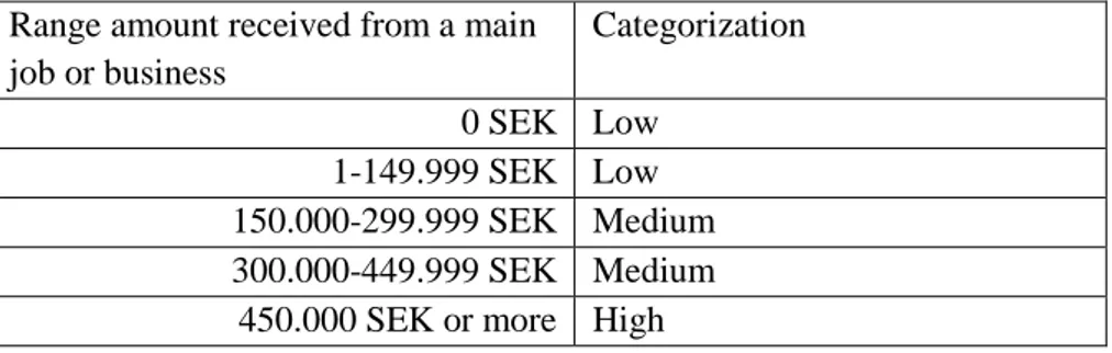
Different aspects of incomes are studied. First, income levels of the female and the male in the couple pre-childbirth, second, the relative income levels within the couple, meaning whether one of the partners has a higher income than the other, and third, the different possible “income constellations” that a couple can fall into. Income levels before and after childbirth were categorized as “high”, “medium”, or “low”, resulting in 9 possible combinations of couples’ incomes. The high, medium, and low categorizations were only used when dealing with income-constellations, otherwise the five raw-data-categories were used.

For the first analysis of income changes, the incomes in W1 and W2 are used instead of incomes the year before and after childbirth since both those with children and those without were compares. This lowers the accuracy of the analysis since it is not an accurate proxy for parental leave or short-term (direct) career penalty. Incomes 2-3 years after childbirth differs from the incomes of the first year the child is alive. It could for instance be the case that some individuals who went on to have a child sometime in between the waves did not have a job in 2012 but that they then gained one before having a child. However, since both those who conceived a first child and those who did not had to be included, using incomes in W1 and W2 was found to be the best alternative.

Some control variables were used such as the age of the female in the relationship, and as for the education variable, a dummy was used signifying having a tertiary education or not. Other circumstances were not controlled for but mentioned as descriptive statistics. Size of the place of birth had to act as a proxy for size of place of growing up or place of residence, in lack of data. We know that where you live/grow up has an impact on timing of births, where women in rural areas tend to have children earlier

(18)

14

than women in urban areas (which is also connected to education levels, income levels), although this effect has been diminishing in recent decades (Jones & Tertilt 2007).

3.2 Method

First, how incomes relate to fertility delay was studied through looking at the fertility behavior of couples that did not have any children in wave 1. Binomial logistic regressions were run on the likelihood of having a child between the waves based on pre-childbirth incomes of the couple, subsequently controlling for female age as well as female education. The dependent variable was a binary variable, taking on the value of 0 if the couple remained without a child between waves, and 1 if the couple had a first child between the waves. This approach assumed that (most of) the couples who do not have a child before wave 1 nor in between waves are delaying childbirth to later in life. Only couples where the woman was between the ages of 18 and 40 in wave 1 were included, since women are naturally restricted in their fertility timing. It is less common for women to have children past the age of 40, and women post-40 who choose not to have children are likely not delaying childbirth to later in life. Rather, it is likely that they do not plan on ever having children, thus this age-restriction was made.

The findings were checked for robustness through controlling for age and education of the female in the couple, as well as checking for multicollinearity between variables using variance inflation factors (see Appendix C: Table 13). Since no VIFs exceeded 1.3, no issue of multicollinearity between the independent variables could be found.

Second, changes in income of couples who conceive a first child between the waves were investigated. In the analysis of relative incomes and for the cross-country comparison multinomial logistic models were used, which are a simple extension of binary logistic regressions. Multinomial models allow for the dependent variable to include more than two categories. In these specific regressions, the dependent variable had three possible outcomes for incomes post-childbirth; 1 signifying an income increase, 2 signifying an income decrease, and 3 signifying that income stayed the same. Category 2, income decrease, was used as the reference category. This means that both categories 1 and 3 were evaluated in relation to category 2.

For the analysis of income constellations, a multinomial regression would have been difficult to interpret, which is why in this case a binomial regression was used, where the dependent variable could take on the values of 1 signifying an income decrease, or 0 signifying that the income stays the same or increases.

(19)

15

Wald Tests were also conducted for both parts of the study when there was doubt as to the significance of the joint significance of several dummy variables.

3.3 Limitations

The conclusions we can draw from the findings of this study are limited. There could be unobserved heterogeneity where for instance, women who wish to have children early, also choose educations and occupations which are in line with this preference. We cannot conclude any causal relationships using the findings from this study since a more complex model would have to be used. Also, the findings are limited in time to the period between W1 and W2. We would have to assume that there are no differences between cohorts having children in this period and other cohorts. Macroeconomic fluctuations affecting unemployment and incomes for instance are not controlled for or considered in this study.

The assumption that fertility and fertility timing can be used as synonymous is useful but another assumption which must be made makes the analysis a bit less accurate. Although fertility historically has been tied to fertility timing, it does not mean the two concepts are inherently linked to each other. Perhaps a delay of first child is will not lead to fewer children overall. It is possible to imagine that those who wish to have children will have a first child whatever time they prefer and that subsequent children then are a question of opportunity cost. After the first child, the marginal utility decreases and they may increase quality of children instead of having more. Thus, focusing on timing of fertility means we must stretch to draw conclusions about fertility.

The fact that the raw income data was categorized instead of providing the specific earnings figures was a limitation. This meant that observing movements in income became more difficult since some individuals are close to the bounds of the categories while others are not. Also, it is arguably easier for people who earned 0 SEK in wave 1 to increase in income level (earn more than 0 SEK) than it is for those in higher income categories to move to another. Categorizing these incomes further into three levels (high, medium, low) decreased accuracy further. The analysis is also made less accurate through excluding certain couples from the analysis. The study does not consider adopted children although it could be said that they in most ways are like biological children in their implications for couples (parental leave, costs, entry into parenthood etc.). Homosexual couples and those without a partner were also not included. This could be bad in terms of accuracy since we do not include the people who get a partner after wave 1 and then proceed to have a child with them before wave 2.

Another limitation is the limitations connected to the response rate (58.8 percent for the Swedish GGS), or rather the non-response rate, which could lead to sampling bias. If the people opting to not answer the survey are disproportionally a certain type of people, the sample is not reflective of the population.

(20)

16

The German data had many limitations, and thus interesting cross-country comparisons could not be conducted, such as studying fertility delay. The analysis could not be done as comprehensively as for the Swedish data due to the structure and availability of data; we only observe income levels at the time of the two waves and not every year in between as in the Swedish data. Thus, income from waves 1 and 2 had to be used as proxies for incomes the year before and after childbirth, which lowers the accuracy of the analysis. Incomes 2-3 years after childbirth differs from the incomes of the first year the child is alive. This applies also to the parts of the Swedish findings which use incomes from W1 and W2. Thus, those findings should be analyzed as semi-long term for some of the couples and short-term for others, but no distinction can be made. The German GGS data also has the issues of non-response as already mentioned, but also issues of attrition rate between the two waves (68 percent), which is not the case for in the Swedish sample.

The results on income changes implicitly assumes that everyone who did not have a child will have the same or increased incomes in wave 2 compared to wave 1, but this is likely not the case due to different factors, the most important being unemployment. Hence, this assumption makes the results especially vulnerable to temporary macroeconomic fluctuations. It would thus have been preferable to either use couples who did not have a child between waves as a control group to make the results more robust, or to increase the time scope of the study to account for fluctuations over time.

(21)

17

4. EMPIRICAL FINDINGS

The empirical findings of the study are presented in this section. The findings are divided into three main sections. The first presents the findings about the couple’s incomes and their likelihood to delay fertility. The second is about how the income levels change for the couple post-childbirth and how that is related to their pre-childbirth income levels. The third is a cross-country comparison of Swedish and German income changes pre- and post-childbirth. Each section includes both descriptive statistics and regression results.

4.1 Fertility delay and incomes

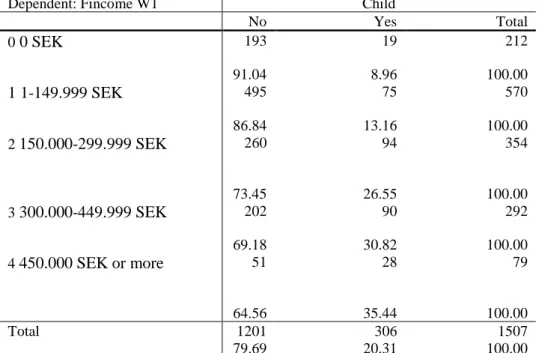
In the section checking for fertility delay, the dependent variable was a dummy with two possible outcomes having a child (1) or not having a child (0) in between the waves. Doing a simple tabulation of the incomes in wave 1 and having a child or not in between the waves, we can see that the higher the female income was in wave 1, the more likely she is to have a first child between the waves. 35.44 percent for those in the highest income category went on to have a child, compared to 8.96 percent for those in the lowest category (See Appendix C: Table 1). The same pattern can be seen among the males. 34.87 percent for the highest income group went on to have a child, compared to 3.55 percent for the lowest income group (See Appendix C: Table 2). Naturally, this is just an overview and does not consider differences in age, education, place of birth, nor partners’ incomes.

Women with a tertiary education in the data had a median age at first birth of 30 compared to 27 for women without a tertiary education. If the male has a tertiary education, his female partner’s median age at first birth is 30, and 28 if he has no tertiary education (See Appendix C: Table 3 and 4).

Both women born in cities and more sparsely populated areas of Sweden had a median age at first birth of 29 (See Appendix C: Table 5). But being born in a city was associated with about 10 and a half months (0.87 year) later age at first childbirth (See Appendix C: Table 6).

We will control for female education and female age when running our main regressions, but not for being born in a city since this was not found to be significant in any of the regressions and since its impact has been found to be diminishing in recent decades (Jones & Tertilt 2007).

4.1.1 Female and male incomes

To check for multicollinearity, variance inflation factors (VIF) were computed on combinations of the independent variables. Since none of the variables in any of the regressions on fertility delay and income

(22)

18

resulted in VIFs above 1.3, there was no issue of multicollinearity between independent variables (see Appendix C: Table 13).

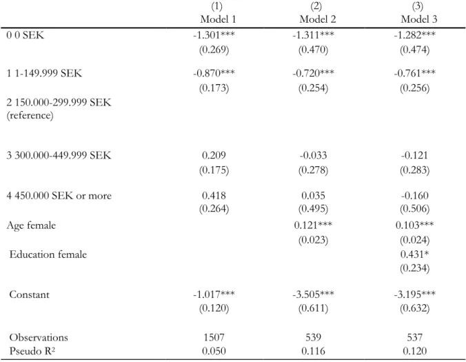
We check the likelihood of having a child in the period between the two waves and its relationship to the pre-childbirth incomes of the couple. Using a binomial logistic regression with female age, female education, and incomes in W1 as dependent variables we find that male income is associated positively to likelihood of having a child, as well as the female having a tertiary education. Female income in W1 and female age are not found to be significant (see Appendix C: Table 7). Delving deeper into the male and female incomes as explanatory variables for fertility delay, a number of logistic regressions on the likelihood of having a first child were run. In the first regression, the independent variables of most interest were the female income in wave 1 with income category 2 (middle one) as the reference category, controlling for age and education (see Table 1 – Model 3). Doing this we can observe a relationship between female income and fertility delay in which couples are more likely to delay childbirth when the womans income is in the two lowest income categories. The coefficient for female age is slightly positive, indicating that as women get older they are less likely to delay childbirth. The education coefficient similarly is positive, indicating that having tertiary educaton also decreases likelihood of fertility delay although it is only significant for a confidence level of 90 percent. Since the higher income categories are not significant, we can only conclude that lower female incomes (category 0 and 1) increase the likelihood to delay childbirth compared to category 2. The results do not differ substantially when controling or not controling for age and educaiton (comparing model 1, 2, and 3) (see Table 1 – Model 1-3).

(23)

19

Table 1. Logistic regressions on likelihood of becoming a parent based on female income the year of W1

(1) (2) (3)

Model 1 Model 2 Model 3

0 0 SEK -1.301*** -1.311*** -1.282*** (0.269) (0.470) (0.474) 1 1-149.999 SEK -0.870*** -0.720*** -0.761*** (0.173) (0.254) (0.256) 2 150.000-299.999 SEK (reference) 3 300.000-449.999 SEK 0.209 -0.033 -0.121 (0.175) (0.278) (0.283) 4 450.000 SEK or more 0.418 0.035 -0.160 (0.264) (0.495) (0.506) Age female 0.121*** 0.103*** (0.023) (0.024) Education female 0.431* (0.234) Constant -1.017*** -3.505*** -3.195*** (0.120) (0.611) (0.632) Observations 1507 539 537 Pseudo R2 _0.050 _0.116 _0.120

The dependent variable is a binary variable which can take the values 1 and 0, 1 means having a first child in between waves, and 0 means not having a first child between the waves.

Standard errors are in parentheses *** p<.01, ** p<.05, * p<.1

Source: Adapted from United Nations Economic Commission for Europe (2005)

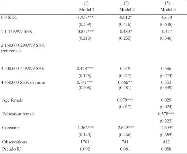
Running the same regression on male income in wave 1, keeping income category 2 as the reference category and still controlling for age and education, we observe no significant difference in likelihood to have a child based on male incomes in W1 (see Table 2 – Model 3). Not controlling for female education we can see a higher likelihood to have a child when belonging to the highest income category, and when not controlling for neither female age nor education, all income levels of the male are significant, showing that the higher the income a man has, the more likely he is to have a child. This can be explained by the fact that income increases with age, this means that men who earn more are often older and subsequently, so are their female partners. The effect of this is removed after controlling for female age, thus we cannot say that male income is significantly affecting likelihood to have a child. We run a Wald Test checking for joint significance of the dummy categories, and find that male income in w1 overall is significant to the model (p-value 0.0186, see Table 3). Since the coefficients of the male income-categories in the logistic regression follow distinct pattern of negative for lower income (than

(24)

20

category 2) and positive for higher income (see Table 2 – Model 3). Thus, we find evidence that male income is significantly positively related to having a child.

Table 2. Logistic regressions on likelihood of becoming a parent based on male income the year of W1

(1) (2) (3)

Model 1 Model 2 Model 3

0 0 SEK -1.937*** -0.812* -0.670 (0.339) (0.416) (0.648) 1 1-149.999 SEK -0.877*** -0.480* -0.477 (0.213) (0.255) (0.346) 2 150.000-299.999 SEK (reference) 3 300.000-449.999 SEK 0.478*** 0.319 0.386 (0.175) (0.217) (0.274) 4 450.000 SEK or more 0.741*** 0.666** 0.553 (0.208) (0.281) (0.349) Age female 0.079*** 0.029 (0.017) (0.024) Education female 0.578*** (0.223) Constant -1.366*** -2.629*** -1.209* (0.143) (0.466) (0.655) Observations 1761 741 412 Pseudo R2 _0.092 _0.081 _0.058

Table 3. Wald Tests of Male and Female Income in the year of W1 (Wald Tests on Model 3 in Table 1

and Model 3 in Table 2)

Male Income W1 Female Income W1

Chi2(4) 11.84 25.86

(25)

21

4.1.2 Relative income and income constellations

Next, the relative income within a couples was used as the main independent variable. Males are on average older than their female partners, and these age differences may also impact the relative incomes within a couple. Surprisingly the largest age gap between the partners is found to be when the woman earns more, the man is on average 4 years older than the woman, while the smallest gap in age, 2 years, is observed for couples where the man earns more (see Appendix C: Table 8). Thus, there is no reason to believe that relative incomes in a couples stems from their age differences.

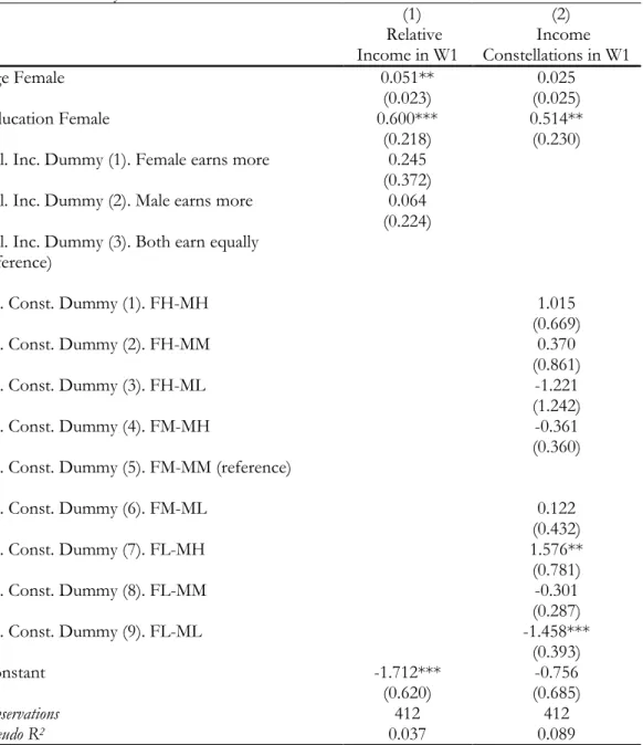
Tabulating relative incomes and the dependent variable, we can see that in this cohort, couples where the male earns more than the woman are the most likely to have a child (40.5 percent), followed by equal incomes (33.5 percent), and the woman having a higher income (29.7 percent) (see Appendix C: Table 9). Running a logistic regression on the likelihood to have a child between waves with relative incomes as the main independent variable. The variable had three possible outcomes: female earns more, male earns more, and partners earn equally (reference category). Doing this, no significant differences in likelihood to give birth for different relative incomes between partners were found (see Table 5 – Model 1). This continues to be the case even when not controling for age and education. The variable relative income as a whole is also not found to be of significance for the model when running a Wald Test (p-value 0.7955, see Table 6).

Table 4. Income Constellations information

Nr. Constellation Name Female income level Male income level

1 FH-MH High High

2 FH-MM High Medium

3 FH-ML High Low

4 FM-MH Medium High

5 FM-MM (reference) Medium Medium

6 FM-ML Medium Low

7 FL-MH Low High

8 FL-MM Low Medium

9 FL-ML Low Low

After categorizing incomes into three levels: high, medium, and low, these subsequently lead to 9 different income categories of income constellations which couples without children in W1 can fall into (see Table 4 above). When tabulating the constellations, couples in FL-MH (7) and FH-MH (1) saw the largest share of couples who went on to have a child, 59.1 and 51.9 percent respectively. The smallest share going on to have a child were in FH-ML (3) and FL-ML (9), 11.1 and 11.6 percent respectively

(26)

22

(see Appendix C: Table 10). We can begin to see a pattern of male income being significant, since male income is high in both constellations which saw the highest level of childbirth (FL-MH and FH-MH), while as the same time being low in both constellations with the lowest levels of childbirth (FH-ML and FL-ML).

When running the logistic regression on income constellations, using FM-MM (5) as the reference group, constellations FL-MH (7) and FL-ML (9) were the only significant ones (see Table 5 – Model 2). When the woman’s income is low and the man’s is high, they are more likely to have a child rather than delay childbirth, compared to when they both have a medium income. When both are low income they are much less likely to have a child compared to when both are medium income. Since constellations FL-MH and FL-ML go in opposite directions and the only difference is that the male income is high in one and low in the other, we can conclude that if the female income is low, the couple is more likely to have a child if the male income is high rather than low.

The Wald test showed that the income constellations are significant to fertility (p-value 0.0019, see Table 6). Looking at the coefficients for each constellation, some patterns seem to emerge. Firstly, considering male incomes, they seem to be positively realted to childbirth when the womans income is low, and less so when it is high (coefficients rising with male income). When the woman’s income is medium however, the relationship seeems to go in the opposite direction (coefficient shrinking with male income, see Table 5 – Model 2). Considering women’s incomes, it is more difficult to make out any noticeable patterns. It seems like when the man earns a high income, low-high-medium seems to be the order of female income which has the most likelihood to least likelihood of childbirth. When the man earns a low income, medium-high-low seems to be the pattern. And with a medium-earning man, fertility is more likely for high earning and less likely for low earning women (see Table 5 – Model 2). From this, we cannot conclude anything about female incomes.

(27)

23

Table 5. Logistic regressions on likelihood of becoming a parent based on relative income and income

constellations in the year of W1

(1) (2)

Relative

Income in W1 Constellations in W1 Income

Age Female 0.051** 0.025

(0.023) (0.025)

Education Female 0.600*** 0.514**

(0.218) (0.230)

Rel. Inc. Dummy (1). Female earns more 0.245

(0.372)

Rel. Inc. Dummy (2). Male earns more 0.064

(0.224)

Rel. Inc. Dummy (3). Both earn equally (reference)

Inc. Const. Dummy (1). FH-MH 1.015

(0.669)

Inc. Const. Dummy (2). FH-MM 0.370

(0.861)

Inc. Const. Dummy (3). FH-ML -1.221

(1.242)

Inc. Const. Dummy (4). FM-MH -0.361

(0.360)

Inc. Const. Dummy (5). FM-MM (reference)

Inc. Const. Dummy (6). FM-ML 0.122

(0.432)

Inc. Const. Dummy (7). FL-MH 1.576**

(0.781)

Inc. Const. Dummy (8). FL-MM -0.301

(0.287)

Inc. Const. Dummy (9). FL-ML -1.458***

(0.393)

Constant -1.712*** -0.756

(0.620) (0.685)

Observations 412 412

Pseudo R2 _0.037 _0.089

Table 6. Wald Tests on Relative Income and Income Constellations (Wald Tests on Model 1 and Model 2

in Table 5)

Relative income Income constellations

Chi2(2) 0.46

Chi2(8) 24.47

(28)

24

4.2 Change in income after having a first child

When looking at a tabulation of income levels pre and post the birth of a first child it is obvious that there is a difference between men and women (see Appendix C: Table 11 and 12). The percentage of women who start off in the highest-income category and who stay there is 4 percent compared to almost 78 percent of the respective men. Correspondingly, out of the females who start off in the lowest income category 85 percent stay low-income post-childbirth while only 36 percent of the males do the same, the rest increase in income. We can see that in couples which have a first child between the waves, female income decreases more often than male income.

4.2.1 Relative incomes

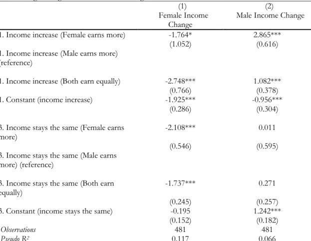
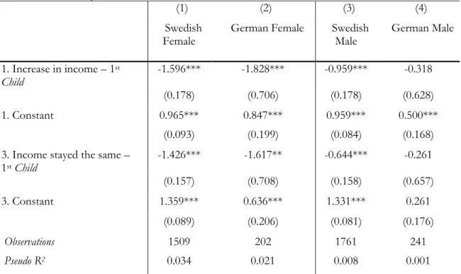
Table 7 describes multinomial logistic regressions on income change where the dependent variable can take on three values; 1 signifying income increase, 2 signifying income decrease, and 3 signifying staying at the same income level. Since category 2, income decrease, was used as the reference category, which is why only categories 1 and 3 are included in the table. Each of these can be seen as a binary logistic regression result in relation to the reference category. Thus, in the case of female income change (Table 7 – Model 1), since the coefficients are significant and negative, this means that the female income is less likely to increase or stay the same (category 1 and 3) than decrease (category 2), given that the woman earns more or equally to her male partner. If she earns less than her partner, she is thus more likely to increase in income than otherwise. For male incomes, a similar relationship is found, although it is weaker (Table 7 – Model 2). Since the coefficients for income increase (category 1) are significantly positive, this means that male income is more likely to increase as opposed to decrease when he earns less or equally to his female partner. Consequently, male income is more likely to decrease rather than increase when he earns more than the woman. We do not get significant results for income staying the same (category 3).

(29)

25

Table 7. Logistic regressions on income change based on relative incomes in W1

(1) (2)

Female Income

Change Male Income Change 1. Income increase (Female earns more) -1.764* 2.865***

(1.052) (0.616)

1. Income increase (Male earns more) (reference)

1. Income increase (Both earn equally) -2.748*** 1.082***

(0.766) (0.378)

1. Constant (income increase) -1.925*** -0.956***

(0.286) (0.304)

3. Income stays the same (Female earns

more) -2.108*** 0.011

(0.546) (0.595)

3. Income stays the same (Male earns more) (reference)

3. Income stays the same (Both earn

equally) -1.737*** 0.271

(0.245) (0.257)

3. Constant (income stays the same) -0.195 1.242***

(0.152) (0.182)

Observations 481 481

Pseudo R2 _0.117 _0.066

The dependent variable is a categorical variable which can take the values 1, 2, and 3. 1 means income increase, 2 means income decrease, and 3 means income staying the same pre- and post-childbirth. Category 2, income decrease is used as reference category for the dependent variable. Standard errors are in parentheses

*** p<.01, ** p<.05, * p<.1

4.2.2 Income categories

Table 8 describes the results of running a binary logistic regression on income change post-childbirth, where the dependent variable was 1 if income decreased, and 0 if income increased or stayed the same. This time using the 9 income constellations as independent variables, immediately before childbirth instead of in W1, and using constellation FM-MM (5) as the reference category. The results show that FH-MH (1), FH-MM (2), and FH-ML (3) predict female income decrease perfectly, indicated by a 1 (Table 8 – Model 1). All women who had a “high” income before childbirth ended up decreasing in income post-childbirth. For clarification, they could not increase in income since they were already in the highest group, but it was possible for them to remain at a high level. The groups which were found to be significantly different from FM-MM were FL-MH (7), FL-MM (8), and FL-ML (9). Women in these groups all earned a low income and were less likely to see an income decrease compared to when both partners earned a medium income. For clarification, it was possible for women in low-income

(30)

26

groups to decrease in income, but they would have to earn 0 SEK for a whole year from main job or business which is unlikely, thus we should perhaps disregard this finding. The findings showed that women in high income segments were very likely to decrease in income, which is as expected.

Running the same regression on male income decrease, the findings indicate that male income decrease is not significant for any income category. However, all men in FH-MH (1), FM-MH (4), and FL-MH (7) saw an income decrease, indicated by a 1. In all these groups the male income is high, thus male income is very likely to decrease when it starts out high, same as for women. Additionally, all men in FH-ML (3) and FL-ML (9) saw no decrease in income, indicated by a 0. The findings indicate that if a man is already low income, he is unlikely to decrease in income post-childbirth, which is also the same result as for the women. The same reservations as for the female income decrease should be had when considering the male income decrease for those starting off in a low-income segment.

Table 8. Logistic regressions on income decrease based on income constellations in W1

(1) (2)

Female income

decrease Male Income decrease

1. FH-MH 1 1 2. FH-MM 1 0.442 (0.686) 3. FH-ML 1 0 4. FM-MH -0.165 1 (0.482) 5. FM-MM (reference) 6. FM-ML -0.927* -1.244 (0.562) (1.045) 7. FL-MH -4.023*** 1 (0.621) 8. FL-MM -3.808*** 0.180 (0.411) (0.345) 9. FL-ML -2.981*** 0 (0.703) Constant 2.576*** -1.646*** (0.277) (0.193) Observations 407 310 Pseudo R2 _0.380 _0.011

The dependent variable is a binary variable which can take the values 1 and 0, 1 means income decreased post-childbirth and 2 means income stayed the same or increased post-childbirth. Standard errors are in parentheses

*** p<.01, ** p<.05, * p<.1