Wind Turbine Production losses in Cold Climate : case study of ten wind farms in Sweden

(1)

1

Wind Turbine Production losses in

Cold Climate

Case study of ten wind farms in Sweden

Author: Jon Kasper Malmsten

Supervisor: Bahri Uzunoglu Examiner: Jens Nørkær Sørensen Program: Wind Power Project Management Department: Wind Energy, Gotland University

(2)

1

Abstract

As wind power expands rapidly worldwide, it is becoming more common to build wind farms in alpine locations where the wind resources often are good and conflicting interests are few. This is evident in Sweden where a substantial portion of the large wind parks planned are to be built in cold climate locations. The fact that icing of turbine blades and sensors can severely impact the production raises the question how large the losses are. In this thesis 10 wind parks comprising 45 turbines, well dispersed throughout Sweden are investigated. Daily production figures are compared to wind data from the MERRA reanalysis data-set in order to see if it is possible to determine the level of losses during the winter period caused by cold climate.

A method is suggested where a relationship between daily production and daily average wind speed is established using representative summer days. This relationship is then used to calculate an expected production for the winter period. Losses are concluded as the difference between expected and actual production.

The method did not produce a consistent and reliable result for the sites investigated. However, the method captures the overall trend with higher losses in the north of Sweden compared to the sites in the south where little or no icing is likely. At the sites where icing is expected, losses in the range of 10 to 20% of the annual production were calculated.

(3)

2

Acknowledgement

I would like to thank my supervisor at Gotland University, Bahri Uzunoglu for appreciated support and reviewing of my work. I would also like to thank Sónia Liléo at O2 for critical reviewing of the method proposed and discussion of possible sources of errors. Also a special thanks to Jonathan Hjorth at Vindstrategi for valuable discussions and ideas.

I am also grateful to the companies and organizations that have provided data for the work. I would like to acknowledge the Global Modeling and Assimilation Office (GMAO) and the GES DISC (Goddard Earth Sciences Data and Information Services Center) for the dissemination of MERRA. The NCEP/NCAR reanalysis data used in this investigation was provided by the NOAA/OAR/ESRL PSD, Boulder, Colorado, USA.

(4)

3

1 Introduction

1.1 Preface

This Master's thesis was completed in partial fulfillment of the Master of Science degree in Wind Power Project Management at Gotland University. The extent of the report is 15 ECTS-credits which is comparable to approximately 10 weeks of full time studies.

1.2 Background

As wind power expands rapidly worldwide, it is becoming more common to build wind farms in alpine locations where the wind resources often are good and conflicting interests are few. The low temperature and the harsh climate in these locations pose new challenges for the wind industry as icing of the turbine blades and sensors could increase the structural loads and reduce production and hence the economical profitability of the investment.

Nowadays it is well known that there may be production losses due to icing in cold climate conditions. In an effort to overcome this, there are a few so-called de-icing systems on the market that uses different methods to heat the blades in order to remove ice that has formed. Anti-icing systems that use hydrophobic coating to prevent ice to accrete on to the blades are also under development.

Some wind assessment companies have, and are developing models that can predict the severity of icing at a selected site. But until now the most common method is to study how the anemometers on the met mast at the sites are affected by icing, which however seems to underestimate the problem (Liléo, O2 2011).

Another challenge is to interpret the icing situation at a specific site into an expected loss in production. No well-defined method or industry standard exists to estimate the losses. Some companies have thoroughly investigated and may have a reasonable estimate of the losses on their farms, but this is generally considered as confidential information and the figures are not shared publicly.

1.3 Problem statement

Speaking to one of the owner of wind farms located in the northern part of Sweden confirms the complexity of the problem: “Production losses are considerable in our northerly located wind farms but we have not calculated how large they are. To calculate the losses is complicated and different types of turbines seem to be differently affected. Some years the losses are small until a single event occurs that shuts down the turbines and induces considerable losses” (Anonymous, 2011).

There are many problems to solve before it is possible to accurately estimate expected losses in production due to icing. The severity and type of ice must be correctly modeled and the effect the ice has on a specific turbine must also be known. It is also complicated to calculate the losses at existing wind farms. However, if this can be done for a wide range of farms it may be possible to establish a relationship between the losses and the level of icing predicted by the icing maps.

(7)

6

1.4 Objectives

The objective of this report is to develop a method to estimate production losses due to cold climate. The method suggested is based on daily production figures from the Swedish national Vindstat database in combination with wind and temperature data from publicly available reanalysis data-sets.

The aim is to implement this method on ten different wind farms dispersed throughout Sweden and investigate if it is possible to conclude the size of the losses.

1.5 Delimitations

This report focuses on the production losses that wind turbines may experience in cold climate. The theory of how and when ice is accreted and the factors influencing the icing are not covered in detail in this report. Neither are the technical solutions for mitigating the icing problem. A short summary of both technical mitigation systems and types of ice is, however, presented in chapter 2.

1.6 Targeted audience

In order to fully understand the content of this report the reader is advised to have some knowledge of the principles behind wind turbines and wind farms. Also some basic knowledge of meteorology is advised.

1.7 Previous work

There are several reports analyzing different aspects of wind turbine applications in cold climates. Many of them focus on how and why ice accretes on the blades (Carlsson 2009), as well as different types of ices and how ice can be modeled (Rindeskär 2010) (T. Laakso 2003). In this chapter, reports focusing on power and production losses are briefly discussed.

In an early work, the effects of rime ice on a 450-kW turbine, operated both under stall-regulated and variable speed mode, where calculated. A computational model was used to predict the effects and losses, which were in the order of 20% for the variable speed rotor (William J. Jasinski 1997). This is however a momentary value that does not predict the total annual loss. In a later work, momentary losses were modeled using a CFD Base solver for a NREL 5MW reference turbine. An icing event was simulated which resulted in power losses of about 27% for wind speeds in the range of 7 to 11 m/s) (Matthew C. Homola 2011).

In an investigation from 1998 annual losses were estimated by analyzing two years of 10-minute turbine data for a test site located at a mountain ridge in the Apennines in Italy (G. Botta 1998). Standard turbines were used which at that time implied that the anemometers on the turbines were unheated. An annual loss was estimated by calculating the expected production during icing events and comparing it with actual production. The calculation was performed using wind data from heated anemometers along with power curves measured during normal conditions. Annual losses in the order of 10 to 20% were found.

(8)

7

In a report from Elforsk in 2009, production losses for a wind park in the far north of Sweden were studied. A power curve for the summer months was concluded by plotting the production in relation to the wind speed using 10-minute turbine data. A ratio between actual and expected power, according to the concluded power curve, was calculated per 10-minute interval for the studied period. Intervals with a ratio below 85% were accounted for as losses. The losses found during the winter period (air temperature below +2 °C degrees) were significantly higher than for the summer; for the period from October year 2005 to March year 2009, the losses were found to be 6.6% during the summer and 27% during the winter (Ronsten 2009).

As part of a national program in Sweden, incidents and operational statistics have been collected and compiled into a national database called Vindstat. During the time in which investment subsidies were given to wind power establishments, production reporting was mandatory. When the electricity certificate system was introduced, the subsidies were removed and also the obligation to report to Vindstat. Many turbine owners are however reporting statistics voluntarily and by end of year 2010 the database comprised approximately 1050 turbines (Nils-Eric Carlstedt 2011). Of all incidents reported in between January 31st 1998 to December 31st 2002, 92 incidents (7%) were related to cold climate, resulting in a 5% loss in production hours (T. Laakso 2003). The number of unrecorded cold climate related incidents can safely be assumed to be significant as the reporting was manual in combination with the lack of technology and methods to detect icing. What is interesting to observe is that 92% of the reported cold climate related incidents were due to icing which emphasizes that the ice, not the temperature, is the main problem.

2 Theoretical framework

2.1 Ice accretion and types of ice

ISO has defined four different ice types resulting mainly from either precipitation or in-cloud icing (Rindeskär 2010):

• Glaze

• Rime (hard/soft) • Wet snow • Hoar frost

Precipitation icing is formed when rain or snow freezes upon contact with a surface while in-cloud icing refers to the deposition of cloud droplets and water vapor on to a surface. In-cloud icing is formed when the elevation of the site is in reach of the cloud base. Hoar frost is formed when water vapor in the air transmutes into ice. In Sweden, atmospheric icing is dominated by in-cloud icing which implies that the elevation of the site is of importance for the ice situation (Carlsson 2009)

Several factors impact the amount and type of ice that will accrete onto a structure, but the most important ones are the air temperature, liquid water content (LWC) of the

(9)

8

clouds and wind speed (higher speed results in a higher ice deposition). The size and shape of the structure is also of importance (Rindeskär 2010).

2.2 Icing in Sweden

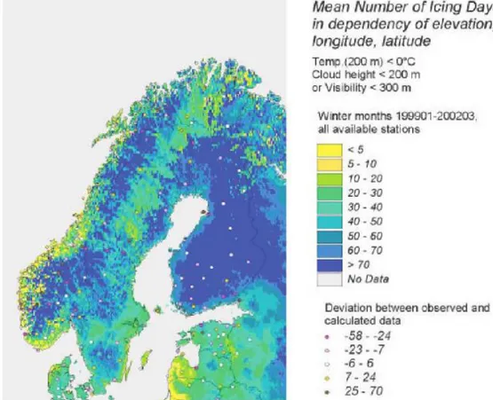
As the prevailing wind direction in Sweden is from southwest, the Norwegian mountains shelter the northern parts of Sweden from most of the moist air coming from the Atlantic Ocean. The mountains, however, provide less protection further south in the county of Jämtland, and occasionally when cold easterly winds flow from the unfrozen Baltic sea, severe icing could affect large areas. The low temperature and solar insolation in northern Sweden during the winter can prevent iced up structures to deice naturally, hence iced up structures can stay iced for very long time (T. Laakso 2003). No recent icing map is currently available for Sweden. The map presented below is from 2003 but it is based on simple criteria and a relative short time period and it is basically unverified. But it gives a general idea of where icing is likely to occur, see Figure 1 below.

Figure 1: Icing map of Scandinavia with estimated number of icing days (Ronsten 2008)

2.3 Icing mitigation systems for wind turbine applications

Most turbine manufacturers provide a cold climate package which, among other things, generally includes heated wind sensors. Systems for blade heating are also being developed and there are a few commercially available options. Enercon uses a system which circulates hot air inside the blades; WinWind uses a system in which carbon fiber elements, mounted near the surface of the blades, are electrically heated. Current

(10)

9

practices indicate that only systems which heat the surfaces of the blades are effective in heavy icing conditions (T. Laakso 2003).

2.4 Wind data

Wind data from the newly compiled MERRA reanalysis data-set was used. MERRA (Modern Era Retrospective-analysis for Research and Applications) is produced by the NASA Global Model and Assimilation Office (GMAO) and covers the satellite era of remotely sensed data from 1979 through present (Lucchesi 2008). Version 5 of the Goddard Earth Observing System Data Assimilation System (GEOS-5) is used. The spatial resolution is 1/2 degree Latitude x 2/3 degree Longitude (56x74 km) and the temporal resolution is one hour.

From the MERRA data-set the 50 meter single-level data product were used and no correction was made to adjust the wind speed to actual hub height at the sites. But when assuming an air stability that does not vary over time the height of the hub can be neglected as the production will be correlated to the wind speed at 50 meter instead of the wind speed at hub height.

For two of the wind farms investigated 10-minute wind speed data from the turbines were available and used as a reference when evaluating the results.

For the MERRA wind data, a daily average wind speed was calculated as the sum of the observed wind speeds during each day divided by the number of observations. 10-minute turbine data was converted into a daily average wind speed by first calculating an average wind speed within the farm for each 10-minute time slot during the day. The average wind speeds for all time slots were then summarized and divided by the number of observations.

2.4.1 Wind direction

Calculating the average wind direction is not a straightforward process. If for example the wind blows half the time from the south and half the time from the north there is no obvious average found; the average could be either east or west. When calculating a daily average direction this is normally not a problem as the wind tends to gradually shift direction, which however assumes a reasonably high sampling rate in order to record the different directions. The fact that the wind direction is measured in a non-continues scale where 0 and 360 degrees refers to the same direction, also complicates the calculation.

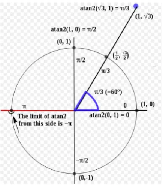
The approach applied in this study was to use the Arctan2 function using the sum of all sampled wind directions’ sine and cosine values as argument according to Equation 1 below. In case the function returns a negative value, the figure 360 is added to the result to conclude a positive degree, see Figure 2 below.

(∑ ( ) ∑ ( )) Equation 1: The average wind direction Dav is calculated using the Atan2 function.

(11)

10

Figure 2: Different values returned by the Atan2 function depending on the angle.

2.5 Air temperature data

Temperature from NCEP/NCAR was used since the MERRA data made available for this project did not include air temperature and it was considered too time consuming to download and decode the MERRA temperature data series. The NCEP/NCAR data-set is a joint production of the National Center for Environmental Prediction (NCEP) and the National Center for Atmospheric Research (NCAR). The data-set is a global analysis covering the period 1948 to present with a horizontal resolution of 2.5 x 2.5 degrees latitude/longitude (275x275 km) (Climate prediction center u.d.). Temperature from the two meter level was used.

The reason why wind data from MERRA was used instead of data from NCEP/NCAR was because of the much higher spatial resolution that likely provides a better representation of the local wind climate. In a recent investigation where wind data from three different reanalysis data-sets were compared to local measurements within Sweden, the MERRA data showed an improvement in correlation of 16% compared to NCEP/NCAR (improvement of the R-value) (Liléo and Petrik 2011).

2.6 Air density

The energy in the wind has a linear relationship to the density of the air; hence the production of a wind turbine is dependent on the air density. This can be concluded by looking at the general equation for power output from a wind turbine, see Equation 2 below (Tony Burton 2008).

(12)

11

Equation 2: Where P is the power of the turbine, is the power coefficient, A is the swept area, U is the wind

speed and is the air density. The density varies with the temperature and the humidity of the air; cool dry air is heavier than warm humid air.

Air density is dependent on relative humidity, temperature and altitude. As the altitude is constant for a wind turbine it can be neglected in this case, see reasoning in section 2.6.1 below. The difference in density between dry and humid air is relative low; for air with a temperature of +20 °C the difference between dry air and air with 100 % relative humidity is approximately 0,9% (at -20 °C the figure is 0,04%). Temperature itself has a larger impact; dry air at -20 °C is approximately 14% heavier than dry air at 20 °C. To simplify the regression analysis all production figures from the turbines were adjusted to a corresponding production at 0 °C. The relative humidity was assumed to be 90% during the winter period and 70% in the summer. Assuming a constant humidity for the different seasons is reasonable, considering the low impact the humidity has on the air density. Using Equation 2 above a linear relationship between the production at 0 °C and the production at a given temperature was derived as:

Equation 3: Where Prod0 is the production at 0 °C, ρ0 is the density of air at 0 °C, ρt is the density of air at

temperature t and Prodt is the production at temperature t.

The Universal Gas Law (Equation 4) is used to calculate the density of an ideal gas. The characteristics of dry air are close enough to those of an ideal gas, therefore the function is applicable for air (Ingvar Ekroth 2006):

Equation 4: The universal gas law. P is pressure (Pa), R the universal gas constant (J/(mol*K)) and T the temperature (Kelvin).

Air density is calculated as the density of dry air plus the density of water vapor at a given temperature and pressure. The universal gas law is used to calculate the

contributions from the air and water vapor:

Equation 5: Where Pd is the pressure of dry air (Pa), Pv the pressure of water vapor (Pa), Rd = gas constant for dry

air (287.05 J/(mol*K)), Rv = gas constant for water vapor (461.495 J/(mol*K)) and Tt is the temperature in Kelvin.

To calculate the pressure of water vapor (Pv) the saturation water pressure must first be determined. There are several algorithms for calculating the saturation water pressure. The following formula offers satisfying accuracy (Ingvar Ekroth 2006):

(

)

Equation 6: Where ES is the saturation pressure of water vapor (bar), Tc the temperature (°C) and e the base of

(13)

12

The pressure of water vapor is calculated as (Ingvar Ekroth 2006):

Equation 7: Where RH is the relative humidity (expressed as a decimal value).

By using the relationship between the total air pressure P, the water vapor pressure Pv and the pressure of dry air Pd and assuming the total pressure P = 101325 (Pa) (standard air pressure at sea level), the pressure of dry air can be calculated using the following relationship:

Equation 8: Relationship between the total pressure P, pressure for dry air Pd and water vapor pressure Pv..

Combining all formulas gives the following relationship between air density and temperature: ( ) ( )

Equation 9: Function for calculating the air density at a given temperature. RH is the relative humidity, Tc the

temperature (°C), Rd the gas constant for dry air (287.05 J/(mol*K)), Rv the gas constant for water vapor (461.495

J/(mol*K)), Tt the temperature in Kelvin and e is the base of the natural logarithm.

2.6.1 Air density and altitude

As the altitudes of the turbines are constant the altitude can be neglected when calculating the production losses. If the Universal Gas Law (Equation 4) is combined with Equation 3 the following relationship can be concluded:

( ) ()

Equation 10: Deriving that the pressure at a specific altitude does not impact the relationship between the productions at two different temperatures. This however implies that the pressure on the specific altitude is constant.

When assuming dry air the pressure at the specific altitude of the turbines can be neglected as depicted in Equation 10 above. However, when the relative humidity is included in the equation, the pressure cannot that easily be removed. So to fully investigate in the impact, the difference in density ratio of air at 0 °C and 20 °C between sea level and the altitude at 500 meter using a relative humidity of 90% has been calculated. The difference in ratio was less than 0.04% which is negligible in this case.

2.7 Polynomial regression fit

A polynomial regression is a non-linear regression where the relationship between a dependent variable y and the independent variable x is modeled as an nth order polynomial (Ejlertsson 1992). In this work a polynomial of second order is chosen as it is believed to adequately represent the exponential behavior of the relationship between

(14)

13

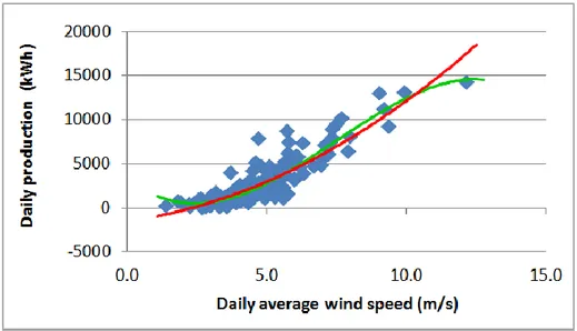
average wind speed and production. An alternative option would be to use a polynomial of third order to better capture the behavior of the production leveling out for higher wind speeds as a result of the turbine reaching its rated power. But in some cases a polynomial of third order has resulted in an unrealistic trend line where the production is abnormally decreasing for high wind speed and increasing for low winds, see Figure 3 below. This is not a problem as long as the studied wind speeds are within the plotted range, but if the relationship is applied to higher wind speeds, a production level that is too low may be concluded. This is further discussed in section 3.4.4 below.

Figure 3: A second (red, bow shaped) and third (green, s-shaped) order polynomial trend line is fitted in a plot of daily production vs. daily average wind speed. Source: by author

3 Method

Daily production data for ten wind farms located in different areas of Sweden were compared to daily wind reanalysis data from the MERRA data-set. Using figures from May to September, a relationship between the average daily wind speed and the daily production was established for the different wind farms. Using this relationship, the expected production for the rest of the year was calculated and compared to the actual production. The difference between calculated and actual production was analyzed in an effort to conclude production losses during the winter.

The reference summer period from May to September was selected because the average minimum 24 hour temperature for this period is above zero degrees for all the areas where the studied wind farms are located (SMHI n.d.).

3.1 Production data

Production figures from the national database Vindstat were used, which represents production figures from the majority of Swedish wind turbines. Since 2002 the reporting has been automated which has increased the quality of the data. In addition to production figures, the database also contains general information about the turbines such as location, rated power, manufacturer etc.

(15)

14

Days where no communication was recorded between the turbines and the database were filtered out when establishing a correlation between production and wind speed, see Table 1 below. For two wind farms, ten minutes data from turbines were used instead of data from Vindstat to calculate the daily energy production.

Table 1: Screenshot of the database where three days are marked with “Beräknat = 1” indicating that no connection could be established between the database and the server for those days. When a connection is established again, the production is distributed evenly over the days where no connection was established.

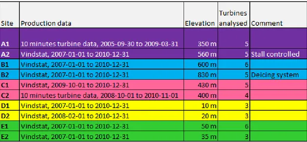
3.2 Studied wind farms

Currently the Vindstat database contains more than one thousand turbines, which was beyond the scope of this report. The method employed in this study was to find newer pitch regulated turbines, well distributed throughout Sweden, with available production figures from year 2007 and onwards. Only wind farms with at least three turbines of the same size and model have been studied as it is much easier to filter out days where a turbine is fully operational if reference turbines are closely located.

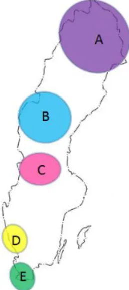
In practice, however, it was difficult to find turbines that fulfilled all of the criteria. One wind farm with stall regulated turbines is therefore included and for three farms production data for the whole period was not available. Altogether ten wind farms were studied comprising forty-five turbines located in five areas well distributed throughout Sweden, see Figure 4 below.

(16)

15

The wind farms in the far south (area D and E) are not believed to have too much of production losses due to icing as the climate is fairly mild, but for the areas A, B and C production losses are likely.

Table 2: Summary of the wind farms studied. The letter defines in which area the turbine is located (wind farm A1 and A2 are located in the area A marked in Figure 4). Source: by author

At site A1 two turbines were excluded from the investigation as they lacked data for a substantial portion of the period studied. An alternative would have been to just exclude the days with missing data. At site B1 one turbine was excluded from the study as it had some long periods (over a month), both during the summer and the winter where no production data was reported.

3.3 Correlation

To analyze general trends, the correlation between production and wind speed during thesummer month was compared to the correlation during the winter. Actual production figures were recalculated to a corresponding production at 0 °C and plotted for the winter and the summer months respectively. By fitting a second order polynomial regression line to the plot, the R-squared value for the fit was concluded. Days when no connection was established between Vindstat and the turbines were discarded. The R-squared value is a number from 0 to 1 that tells how closely the trend line corresponds to the actual data. A trend line is most reliable when its R-squared value is at or near 1.

3.4 Production losses

To investigate the possibility to determine production losses for the winter period an expected production was calculated for the winter and compared to the actual production retrieved from the Vindstat database. For each wind farm, daily production figures from Vindstat and daily wind speed figures from the closest MERRA data point were plotted for representative summer days (see section 3.4.1 about how the representative summer days were selected). A second order polynomial trend line was fitted to the plot and the production as a function of wind speed was established. Using the function defined for the representative summer days, the expected production for the

(17)

16

remaining days could be calculated. An overview of the procedure is presented in Figure 5 below.

Figure 5: A schematic overview of the steps taken to calculate the expected production. Source: by author. 3.4.1 Representative summer days

Representative summer days were found by first studying the different turbines’ contribution to the total production of a wind farm. For every day the turbine with the highest production was found and used as a reference to calculate the share of each turbine’s production. Only days where the production from at least one other turbine was within 70% of the highest producing turbine were included. Days where no such turbine was found were discarded as it is probable that the other turbines have not been fully operational and it is then impossible to judge if the highest producing turbine also might have been partly shut down during the day. 70% is chosen as it is fair to believe that the two turbines within a wind farm that has the highest daily production produce within 70% of each other, if fully operational.

For all summer days that qualify, the production of each turbine is calculated as a fraction of the highest producing turbine (a number from 0 to 100%). For every turbine, an average and a standard deviation of the calculated fraction is concluded. In Table 3 below an example is presented where turbine T1 for day 2007-05-01 produces 97% of the highest producing turbine. On average turbine T1 produces 93% of the daily maximum and the standard deviation is 11%. Day 2007-05-03 not maximum is calculated as there is no production that is within 70% of the highest producing turbine (T1). Days where a turbine is shut down or no maximum production is found were excluded from the average and standard deviation calculation.

Convert the production for the representative days to a reference density (at temperature 0 °C)

Find representative summer days

Plot and conclude a relationship between daily production and daily average wind speed

Apply the relationship on the winter period to calculate the expected production

Convert the expected production using the actual temperature of each day

(18)

17

SD: 11% 4% 8% 8%

Turbines Average: 93% 92% 92% 94%

date ws temp T1 T2 T3 T4 Max S1 S2 S3 S4

2007-05-01 6,4 0,2 2939 2683 2858 3032 3032 97% 88% 94% 100%

2007-05-02 6,1 -2,8 5117 4872 5436 4300 5436 94% 90% 100% 79%

2007-05-03 5,1 -1,7 1344 500 500 500 FALSE FALSE FALSE FALSE FALSE

2007-05-04 5,5 -2,4 2939 3400 2858 3032 3400 86% 100% 84% 89%

2007-05-05 5,1 -1,7 2434 2605 2910 2935 2935 83% 89% 99% 100%

2007-05-06 5,5 -2,4 719 995 892 1092 1092 66% 91% 82% 100%

Table 3: Production figures for four turbines (T1-T4) during six days are presented together with calculated average production and standard deviation. Note that this is just an example where six days are presented; when including more days the standard deviation is in general higher. Source: by author

The average and the standard deviation were used to determine whether the production of a certain turbine during a specific day shall be included when plotting the relationship between production and wind speed. In order for a turbine to be included during a specific day, the production shall be higher or equal to the calculated average share minus 1.5 times the standard deviation. The threshold value of the average minus 1.5 standard deviations is chosen as that will include about 93% percentages of all samples (assuming a normally distributed data-set). This seems to be a reasonable value as the variation is found to be fairly normally distributed and as it is slightly below the expected availability of a wind turbine (approximately 95% or higher).

For turbine T1 in Table 3 above, only days where the production is higher or equal to 76% (93%- 1.5 x 11%) are included, hence day 2007-05-06 is excluded.

Days where no connection could be established between Vindstat and the turbines were also excluded.

3.4.2 Air density

The production of a wind turbine is dependent on the density of air which in turn depends on the relative humidity, temperature and the altitude. To simplify the regression analysis all production figures from the turbines were adjusted to a corresponding production at 0 °C using a relative humidity of 90% for the winter and 70% for the summer period. The elevation of the turbines can be neglected as it is constant over time. See section 2.6 for further details regarding the air density calculations.

3.4.3 Wind direction

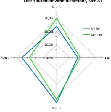
The wind directions were divided into sectors and an individual plot between production and wind speed was done for each sector. This is of importance as the production of the turbines depends on the wind direction, which is mainly due to terrain effects and the influence of the wakes created by the neighboring turbines. As the distribution of the wind directions varies over the year, not taking this into consideration might pose a possible error in the calculations. In Figure 6 below the distribution of wind direction at site A1 is depicted for the summer and the winter period respectively.

(19)

18

Figure 6: The distribution of wind directions for site A1. Summertime, roughly 30% of the days the wind blows from sector North. During the winter, westerly winds are more pronounced. Source: by author

In the figure below, daily production figures for site C1 are plotted for the sectors South and West. At a wind speed of 6 m/s the plot for sector West shows a considerably higher production (approximately 40 000 kWh) compared to sector South (approximately 33 000 kWh)

Figure 7: Plot of daily production as a function of average daily wind speed for two wind sectors at site C1. Source: by author

Following four sectors were defined:

 North: 315 degrees <= Wind direction < 45 degrees

 East: 45 degrees <= Wind direction < 135 degrees

 South: 135 degrees <= Wind direction < 225 degrees

 West: 225 degrees <= Wind direction < 315 degrees

3.4.4 Implication of higher wind speed during the winter compared to the summer As the average wind speed in Sweden is higher during the winter than in the summer, the relationship between wind speed and production concluded for the summer is on

(20)

19

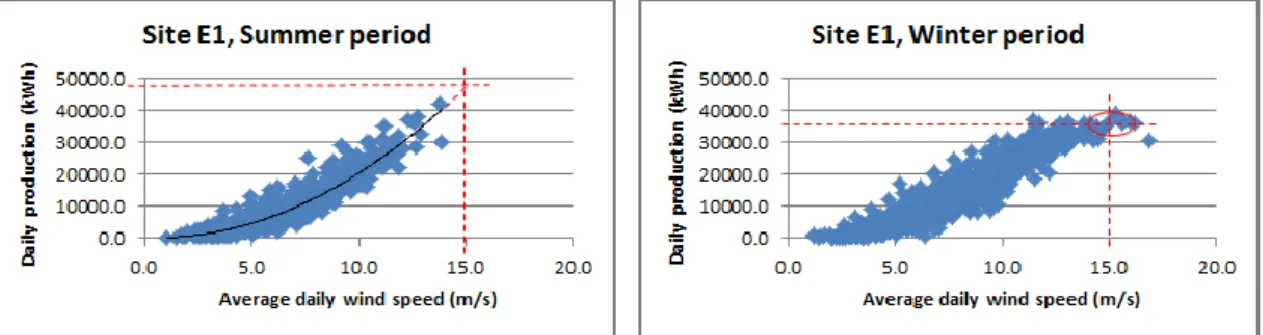
average determined for lower wind speeds than the winter offer. During the winter, the turbines will more often reach their rated power and thus the production curve will flatten out. As a result, using the summer fit for higher wind speeds might lead to an overestimation of the expected production and hence overestimate the losses. In Figure 8 below summer and winter production is plotted for wind farm E1 in the south of Sweden. Studying the trend line for the summer diagram, the production at a wind speed of 15 m/s is estimated at close to 50,000 kWh/day. But when looking at the diagram for the winter plot, the estimated production is somewhere between 30,000 and 40,000 kWh/day for the same wind speed.

Figure 8: Plot of daily production vs. average daily wind speed for the summer and the winter period respectively. The plot is for wind farm E1. Source: by author

To mitigate the impact of this problem, the losses were calculated using only days where the average wind speed were within plus two standard deviations of the total average summer wind speed. The use of two standard deviations is to assure that the average wind speed of the days analyzed are well within the wind speed that the plot represents. Note that the average and standard deviation is calculated for all wind directions; an alternative would have been to make a separate calculation for each of the four wind sectors.

3.4.5 Calculating production losses

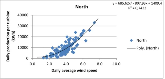
Before fitting the trend line, outliers were visually spotted and removed. On average less than one observation per wind farm and wind sector were removed. In Figure 9 below an example is presented where daily production is plotted as a function of wind speed for the wind sector North.

(21)

20

Figure 9: Daily production and average daily wind speed is plotted for each wind sector (North in this example). Source: by author.

For each day an expected production level was calculated by applying the daily wind data (wind speed and direction from the MERRA data-set) to the concluded relationships between wind speed, direction and production. The daily expected production was adjusted for the temperature given by the NCEP/NCAR data-set. The annual expected production was calculated as the sum of the expected production of all days, reduced by the availability of the turbines.

For the sites reporting production data to the Vindstat database the availability was calculated based on readings from the turbines’ downtime counters which are stored in Vindstat. For the other sites (site A1 and C2) the availability was calculated as the difference between expected and actual production during the summer months:

Equation 11: Calculation of availability. Where As is the availability, Pas is the actual production during the

summer and Pes is the expected summer production.

The losses for the winter period were calculated as:

Equation 12: Function for calculating the annual losses. Pe is expected annual production, As is the calculated

availability for the summer month, Pa is actual annual production and Pl is the loss.

Note that the expected production is reduced by the availability; therefore Pl refers to losses in excess of what is lost due to the availability of the turbines.

3.5 Tools used

A SQL database was constructed to host all data. Preprocessing of the data, such as converting 10-minute turbine data to daily averages, calculating average wind direction, adjusting for time zones etc. was performed in the database. After this process, the data

y = 685,62x2_{- 807,93x + 1409,4} R² = 0,7432 0 10000 20000 30000 40000 0.0 2.0 4.0 6.0 8.0 10.0 D ai ly p ro d u ction p e r tu rb in e (k Wh)

Daily average wind speed North

North Poly. (North)

(22)

21

was further modified an analyzed using Excel; VB-scripts were constructed to modify the air density and the regressions between production and wind speed were concluded using the trend line fit provided in the Excel graphs.

4 Results and analyses

4.1 Correlation

If icing reduces the production during the winter, the correlation between production and wind speed ought to be lower for the winter months than for the summer. As depicted in Table 4 below there is a clear trend demonstrating that the correlation is lower for the winter period in the northern areas, both comparing with corresponding summer period, but also in comparison with the winter correlations of the southern areas. If area D is excluded, a trend is also that the correlation for the summer is lower in the north compared to the south of Sweden. A reason might be that the climate and the terrain represented by the MERRA grid points used for regions A, B and C differ from the local climate and the terrain at the corresponding wind farms as the landscape shows larger variations in these regions compared to regions D and E

It is notable to observe that it is not possible to draw any conclusion regarding how the distance between the wind farm and the MERRA grid point affects the correlation. As reported by Liléo and Petrik (2011) the correlation generally decrease as the distance increases, but it seems as other factors, such as complexity of terrain and local climate, plays a more significant role in this case.

Table 4: R squared value (R2) for the different wind farms using a polynomial fit of second order. Source: by author.

The method was impossible to apply on area D as the correlation between production and wind speed was too low during the summer period, see Table 4. The summer correlation for site D1 of R2 = 0.66 is misleading as the correlation was very high for

(23)

22

westerly winds (R2 = 0.89) but almost nonexistent for northerly winds (R2 = 0.03). A possible reason for the low correlations is the proximity to the sea; the turbines are probably influenced by the sea breeze in a way that is not recognized by the MERRA grid point, located further inland. The fact that the winter period (where the sea breeze is nonexistent) shows a much stronger correlation supports this theory. For site D2 the correlation (R2 = 0.45) is, however, weak also during the winter and therefore other explanations are needed. This has not been further investigated, which is why site D1 and D2 were excluded from further analysis.

The calculated annual loss varies from 19.0% at site B2 to a negative loss of -4.8% for farm C1 indicating that the actual production during the winter is higher than the expected production. The availability varies between 92.9 to 98.5%, see Table 5 below. For the two wind farms in the south (E1 and E2) the losses are as expected close to zero which implies that the method is working fairly well at those sites. But when studying the results at the other sites, especially in area C, the results are not that uniform. For site C2 there is for example a considerable difference in losses when comparing the results achieved by using turbine wind data with the results from when wind data from the MERRA data-set is used. For site A1 no such trend can be seen.

Also of notable importance is that farm B2, which has the highest calculated loss (19.0%), is the only wind farm in this investigation equipped with a blade heating system.

Table 5: Calculated losses and availability for the different sites. Note that the availability for site A1 and C2 is calculated using expected summer production in relation to actual summer production. Source: by author 4.2.1 The impact of daily averaging

In the cases where MERRA wind data was used, the data was averaged from hourly values to a daily average value by summarizing the wind speed measurements during

(24)

23

one day divided by the number of observations. In the same way 10-minute wind data from the turbines were averaged to a daily wind speed value. But as the energy in the wind varies with the cube of the wind speed, two days with the same average wind speed might offer a different amount of energy. If the period studied is long enough and the variation of the energy as a function of the daily average wind speed is randomly distributed over the year, the impact on the loss calculation is probably small. But if instead the wind speed has a seasonal pattern with e.g. more shifting winds during the summer than in the winter, this could induce a significant error when calculating the losses.

To investigate the possible size of this error, 10-minute data from site A1 and C2 were used to calculate the energy content per day. For each 10- minute period the average wind speed within the wind farm was calculated and cubed to represent the energy equivalent for this time slot. The energy equivalent of all 10-minute periods in a specific day were summarized to a daily value and averaged (an average value was used instead of the total sum because some days lacked data for some of the 10-minute time slots). The energy equivalent was also adjusted to a simple power curve assuming the following:

 0-3 m/s => no energy calculated as typically the cut in wind speed is over 3 m/s

 3-4 m/s => the energy equivalent was multiplied with the efficiency factor 0.15

 12-25 m/s => the energy equivalent was calculate for 12 m/s and multiplied with the efficiency factor 0.4

 >25 => No energy was calculated.

The average 10-minute energy equivalent and daily average wind speed was plotted using data for the summer period and a second order polynomial regression line was fitted into the plot, see Figure 10 below. Using this relationship, an expected energy equivalent for the winter period could be calculated and compared to the actual energy equivalent found by summarizing the energy equivalent for each 10-minute slots.

(25)

24

Figure 10: Daily average 10-minute energy equivalent and average daily wind speed plotted. Source: by author. For site A1 the sum of the 10-minute values for the winter period was 2.1% higher than the energy equivalent calculated using the regression fit concluded for the summer period. The corresponding figure for site C2 was 0.7% lower. Only days where the average daily wind speed was within the summer average plus 1.5 standard deviations were considered in the calculation as this is the procedure when calculating the losses. As the method used to calculate the losses assumes the energy to be the same at a given wind speed, this will underestimate the losses at site A1 and overestimate the losses at site C2. The size of the error should be in the range of the calculated difference above (-0.7 to + 2.1%). This is however only calculated for two sites so the impact must be further analyzed to conclude any trends and a general size of the error.

4.2.2 Difference in loss using MERRA wind data compared to turbine wind data For site C2 there is a significant difference in calculated annual losses when the MERRA wind data is used (-0.3%) compared with the loss calculated using turbine data (10.3%), see Table 5. A possible explanation could be that the MERRA wind data in relative terms presents a lower wind speed for the winter than for the summer period, compared to the wind data from the turbines. In Figure 11 below, wind data from the MERRA data-set and the turbines are presented as the monthly average divided by the annual average and plotted as a fraction for each month. A clear trend is that MERRA reanalysis data, in relative terms, assumes a higher wind speed for the summer period and a lower wind speed for the winter period, when compared to the values from the turbines.

Concluding a relationship between the wind speed and the production when the wind speed is overestimated and applying it to a period when wind speed is underestimated will underestimate the losses. The reason why the MERRA wind data has a slightly different seasonal pattern than the wind data from the turbines has not been further investigated but a possible explanation is that local effects at the site influence the wind

in a way that is not recognized by the MERRA data-set. .

y = 6.2461x2_{- 24.974x + 28.853} R² = 0.9859 0 100 200 300 400 500 600 700 0.0 5.0 10.0 15.0 D ai ly av er ag e 10 -m in en er gy e q u iv al e n t

Daily average wind speed (m/s)

Site C2, Summer period

Summer Poly. (Summer)

(26)

25

Figure 11: Comparison of wind speed from the MERRA data-set with wind speed from the turbines at site C2. Monthly average wind speed is divided with annual average and the fraction is plotted for each month. Source: by author.

The losses concluded using the turbine data are probably more accurate than when using MERRA wind data and the value (10.3%), when comparing to the losses estimated for the other sites, seems to be a more realistic value. It should however be noted that the wind farm at C1 uses wind data from a different MERRA grid point so the reason for the low negative loss of -4.8% for this site is unknown.

4.2.3 Sensitivity analysis – Availability

For the two sites (A1 and C2) where the availability was calculated based on the expected and actual summer production the accuracy is questionable due to two reasons: first the calculation itself may be inaccurate; second the assumption that the availability is the same for the winter as for the summer may be wrong. In order to estimate the possible error the availability has also been calculated for the other sites and compared to the figure from Vindstat. On average the absolute difference between the calculated summer availability and the winter availability found in Vindstat were 1.2% with a highest difference of 3.1% for site B2, see Table 6 below.

It is also of importance to mention that it is not known how the turbines calculate the availability. It may well be that some errors caused by icing (e.g. if a turbine shuts down due to low temperature or vibrations caused by icing) is recorded as downtime which in this case will underestimate the losses. To further investigate this issue, the error codes that are classified as downtime has to be known for the turbine models investigated.

80% 90% 100% 110% 120% wi n d sp e e d ; m o n th ly av e rag e /an n u al aver ag e Month MERRA Turbine

(27)

26

Table 6: Calculated availability using expected production compared to actual production for the summer period compared to the availability of the wind farms according to the Vindstat database. Source: by author.

In Table 7 below, the availability has been increased with 1% and the losses recalculated using the increased figure. As depicted, 1% percent higher availability increases the calculated losses with in average 0.95%.

Table 7: The impact the availability has on the losses is studied by increasing the estimated availability with 1%. Source: by author.

Translating this into days means that if all turbines within a farm, for whatever reason, are shut down for 3.6 days during the winter (1% x 8760 (hours per year) divided by 24 (hours per day)) the calculated losses for this year will increase with in average 0.94%. Or if the wind farm consists of five turbines producing evenly, one turbine shut down

(28)

27

for 18 days (3.6 x 5) will give the same result. This is however a theoretical value; if the turbines happens to be shut down when the wind is low, the calculated and real losses will be lower and the opposite if the wind is high.

4.2.4 Sensitivity analysis – temperature

For site A1 and C1 where air temperature data from the turbines is available, the correlation between NCAR temperature and turbine temperature were analyzed.

For site A1, the average annual temperature for year 2006 according to NCAR was -0.2 °C whereas the average measured by the turbines was 5.2 °C, which is considerably higher. But as the NCAR temperature well follows the temperature variations at the site the correlation is high, with an R-squared value of 0.95 for a linear correlation, see Table 8 below. The distance between the site and the NCAR data point is approximately 80 km and the elevation of the site is about 100 meters higher than for the data point.

Table 8: Air temperature from the NCAR data-set compared to data measured by the turbines at site A1. Source: by author.

At site C1 the NCAR temperature was closer to the temperatures measured by the turbines. The annual average for year 2009 measured by the turbines was 6.2 °C and 4.7 °C using NCAR data. Also at this site the NCAR temperature well depicts the variation at the site, with an R-squared value of 0.95, see Table 9 below. The distance between the NCAR data point and the site was approximately 15 km.

Table 9: Air temperature from the NCAR data-set compared to data measured by the turbines at site C2. Source: by author.

For the two sites studied, the air temperature from NCAR and the turbines seems to be well correlated. But as the actual temperature can differ quite substantially it is of

(29)

28

interest to analyze the impact the offset in the temperature has on the calculated losses. If temperature data from the turbines is used instead of NCAR data, when calculating the losses for site A1, the loss is reduced from 18.6% to 18.2%. For site C1 the loss is reduced from 10.3% to 9.9%.

If instead the temperature for all days was reduced by 5 °C (using data for site B2) no change in the calculated loss was found. This is expected as the temperature only is used to find a relationship between production and wind speed at a reference air density. With a constant error between real and estimated temperature, the reference density will just refer to another temperature than the chosen 0 °C. But if the temperature error varies over the year, with e.g. a larger error during the summer than for the winter, it could impact the calculations.

4.2.5 Atmospheric pressure

When calculating the air density a constant reference pressure is used, but in reality the pressure varies continually over time. If the period studied is long enough and the variation is randomly distributed over the seasons, the possible error will likely be small. But if instead a trend, such as that e.g. the pressure on average is lower during the winter than in the summer, or if the pressure correlates with the wind speed (e.g. the pressure is lower for higher wind speeds) the error could be bigger. To study this impact pressure data from Swedish Meteorological and Hydrological Institute (SMHI) was downloaded and analyzed. Data from two weather stations within each area were studied (see Figure 12 below) and a daily average pressure was calculated by summing the pressure data divided by the number of observations (the temporal resolution of the data was 3 hour).

(30)

29

Pressure data at SMHI is available for the period year 1961 to year 2009 which unfortunately does not cover the whole period studied, expect for site A1.

Equation 4 (section 2.6) demonstrates that the air density is linearly proportional to the pressure so if e.g. the pressure is 5% lower during the winter than in the summer, the losses will in theory be overestimated by 5%. In reality the figure ought to be slightly lower as a part of the production is restricted by the nominal power of the generator rather than the energy content of in the wind. As depicted in Table 10 below the difference in average pressure between summer and winter is close to 0.40% with an annual standard deviation of about 0.34% for the period studied.

Table 10: Average pressure for the summer and winter period respectively. The data is downloaded from SMHI. Source: by author.

For all sites the trend is that the pressure decreases slightly with a higher wind speed, which is demonstrated in the plot of wind speed and air pressure for area B in Figure 13 below. But as the production losses are calculated based on days where the wind speed is within 2 standard deviations of the summer average wind speed the impact of this trend ought to be small.

Figure 13: Correlation between daily average wind speed and daily average air pressure for site B for the whole period studied. Wind data from a MERRA grid point within the area B is used. Source: by author.

900.0 920.0 940.0 960.0 980.0 1000.0 0.0 2.0 4.0 6.0 8.0 10.0 12.0 D ai ly av e rae p re ssur e (h Pa)

Daily average wind speed (m/s) Site B. Wind speed vs. pressure for the period

(31)

30

The biggest difference in pressure between summer and winter was concluded for area B during year 2008 when the average winter pressure was around 1% lower than the average summer pressure. The other extreme occurred in year 2007 in area E where the pressure was approximately 0.4% higher during the winter compared to the summer period. This was the only occasion of the sites studied where the average winter pressure was higher than the average summer pressure.

In summary, not using the real air pressure in the calculations will in most cases overestimate the losses with up to 0.5%, but an underestimation could also be possible. To verify the impact on the loss calculation, the air pressure from SMHI was introduced in the calculations for site A1 where pressure data were available for the whole period studied. The calculated loss in production decreased by 0.4% which is slightly lower than the difference in average pressure of 0.5% between summer and winter for the period studied.

5 Discussion and conclusion

The suggested method was applied on ten wind farms comprising 45 wind turbines dispersed from the south to the north of Sweden. Six of the farms were located in areas where icing is likely (area A, B, C), and four in areas far south where the climate is mild and icing events is expected to be rare (area D, E) see Figure 14 below. Unfortunately two wind farms in the south (area D) had to be excluded from the survey as the correlation between the daily production and the wind data from the available MERRA grid point was not sufficient during the summer period.

Figure 14: The different areas studied and their distribution over Sweden.

5.1 Correlation

When studying the correlation between average daily wind speed and daily production for the sites where icing is expected (area A, B, C), a clear trend is that the correlation is lower during the winter compared to the summer. The same trend does not exist for the sites in the south (area E) where the correlation is more or less the same for the winter and summer. The reasonable explanation is that icing affects the production negatively

(32)

31

in the north during the winter period. Another trend is that the correlation in the north in general is lower compared to the sites in area E in the far south. A probable reason is that the climate and the terrain represented by the MERRA grid points in the north differ from the local climate and the terrain at the corresponding wind farms as the landscape shows larger variations in the north compared to the regions in the south.

For the sites where icing is expected the calculated losses vary from 19 to -5%. When excluding the negative loss of area C the loss is in the range of 10 to 20% of annual production. In the south negative losses in the range of 0.5 to almost 2% have been calculated. As negative losses imply that the turbines during the winter produces more than what is possible, this indicates the imperfection of the method employed.

Overall the method captures the trend with higher losses in the north of Sweden compared with the losses calculated for the southern areas. In Ronsten (2009), using another approach, studying the same time period, relative production losses for site A1 was concluded to be 6.6% during the summer and 27% during the winter – i.e. the losses were approximately 20% higher during the winter compared to the summer. This is close to the annual loss of approximately 19% found in this report. For site A1 it is also promising that the method produces the same result when using MERRA wind data as when using wind measurements from the turbines. This was however not the case for site C2 which is problematic for the proposed method.

It should also be noted that the periods investigated differ for some of the sites as it was not possible to retrieve production data for the desired period for all of the turbines. E.g. for site A1 the winter of 2009/2010 is missing which according to a Swedish wind developer resulted in unusually high production losses due to icing.

5.3 Possible sources of error

There are many possible sources of error involved in this type of synoptic method. The most important errors are:

 Reanalysis wind data is used instead of onsite measurements

 Daily averaging of the wind speed data

 Reanalysis temperature data is used instead of onsite measurements

 The air pressure is assumed to be constant but in reality it varies over time

 For two sites the availability were assumed to be the same during the winter as the calculated availability for the summer period.

5.3.1 Reanalysis wind data

Using reanalysis wind data instead of onsite measurements seems to induce the largest source of error in the method proposed. For site C2 the calculated loss was 10% higher when using wind data from the turbines compared to when using MERRA wind data. For site A1 on the other hand, the calculated loss was the same using turbine wind data as when using MERRA wind data. It should also be noted that the loss calculated using the turbine wind measurements cannot be assumed to be fully correct either as other

(33)

32

sources of errors still could have impacted the outcome. It is also impossible to conclude whether the unrealistic negative loss calculated for site C1 has to do with the wind data as no reference measurements were available.

This indicates a weakness of the method as it is based on a relationship between production and wind speed during the summer being also representative for the winter. Several factors could jeopardize this assumption; e.g. local climate factors such as inversions or thermal activities might be more pronounced during either the winter or the summer. If the stability characteristics of the air differ between summer and winter, the simplification not to recalculate the wind speed to the speed at hub height of the studied turbines may also induce an error.

The size of the error using reanalysis wind data might induce is difficult to estimate but for site C2 it appears to be in the order of 10%. For area D the method was impossible to apply as the correlation between the MERRA wind data and the daily production was too low to establish a relationship between production and wind speed.

5.3.2 Daily averaging of wind speed data

The impact that daily averaging has on the proposed method has been studied for the two sites where 10-minute turbine data were available (site A1 and C2). Using an approach where the daily average wind speeds were compared to the daily energy content for the summer and the winter, an error in the range of 1 to 2% were found, respectively. This is however only concluded by analyzing two sites, therefore further analysis should be done to more accurately estimate the size of this error.

5.3.3 Reanalysis temperature data

Using reanalysis data for the air temperature seems not to have any significant impact on the outcome of the calculations. As long as the temperature reasonably well follows the variation at the site, the induced error is small. For the two sites (A1 and C2) the calculated annual loss was reduced by 0.4% when using temperature measurements from the turbines instead of NCEP/NCAR data.

5.3.4 Turbine availability

For two sites (A1 and C2) the availability was calculated by comparing actual and expected production during the summer and assuming the availability to be the same for the winter. By studying the other wind farms where the availability could be calculated using figures from the Vindstat database, this approach induces an error in the range of +/- 1% with a highest reading of approximately 3%.

5.3.5 Assuming constant air pressure

When studying the average air pressure for the areas investigated, in general the pressure was about 0.5% lower during the winter than in the summer. For a single year the difference in pressure was up to 1% lower during wintertime. And for area E in the south, the pressure was 0.4% higher during one winter than in the summer. So in general the losses will be overestimated with close to 0.5% but for single years the size