Kravställning och uppföljning av ljud- och vibrationskrav vid fordonsupphandling

www.vti.se/publikationer

Transportforum 2013

Granskade artiklar

Förord

Vid Transportforum 2013 gavs deltagarna chansen att lämna in ett manuskript för vetenskaplig kvalitetsgranskning. De inkomna bidragen granskades av ledamöter i respektive ämneskommitté. Av de drygt 40 intresseanmälningarna var det nio stycken som fullföljde processen fram till publicering som sker i föreliggande rapport (VTI rapport 787 ”Transportforum 2013 – granskade artiklar”).

Granskningen genomfördes genom att de utsedda granskarna fyllde i ett formulär där artikelns originalitet, struktur, innehåll och nytta samt möjlighet till implementering av resultaten bedömdes. Detta kompletterades med generella synpunkter och

detaljkommentarer från granskarna till hjälp för artikelförfattaren som efter att

granskningsprotokollen anonymiserats fick ta del av dessa och då avgöra om de ville gå vidare med publiceringen.

Transportforums breda ämnesområde, som sträcker över många discipliner, gör att rapporten innehåller artiklar av olika karaktär och inriktningar.

Författarna ansvarar själva för sina artiklar och granskarnas protokoll ska ses som kvalitetshöjande stöd inför publiceringen. Sammanställningen är utförd av Göran Blomqvist, VTI.

Linköping, april 2013

Innehållsförteckning

Ämneskommitté 1: Transportpolitik och ekonomi

• Torbjörn Stenbeck, Riksrevisionen: Comparing productivity means to measure design-build pay-off. (sid. 7),

• Björn Hasselgren, KTH: Pricing principles, efficiency concepts and incetive models in Swedish transport infrastructure policy. (sid. 22),

• Kjell Jansson, Trafikanalys: Samhällsekonomiskt effektiva banavgifter för allokering av knapp spårkapacitet. (sid. 36),

• Kjell Jansson, Trafikanalys: Steg 2, åtgärder för ökad bankapacitet. (sid. 50) • Karin Svensson Smith, Lunds kommun: Vilka styrmedel är lämpliga för att nå

en fossilbränslefri transportsektor? (sid. 67),

Ämneskommitté 5: Trafiksäkerhet

• Joakim Bengtsson, SWECO: Effekter av två olika FIFÖ-system på huvudgata I mindre ort. (sid. 81),

Ämneskommitté 6: Miljöanpassade transporter och framtidens fordon samt drivmedel

• Martin Almgren, SL: Kravställning och uppföljning av ljud och vibrationskrav vid fordonsupphandling. (sid 98),

Ämneskommitté 7: Gods och logistik

• Maria Öberg, LTU: How to create a transport corridor management – a literature review. (sid. 108),

Ämneskommitté 8: Väg och banteknik

• Rickard Nilsson, SL: Utredning och provning av kostnadseffektiva metoder för bullerminimering av spårfordon. (sid. 122).

COMPARING PRODUCTIVITY MEANS TO MEASURE

DESIGN-BUILD PAY-OFF

The effect of design-build and other procurement decisions and strategies related to owner and contractor working more together has long been a topic of discussion. The cost and quality effects have however often been concluded in qualitative terms based on participants’ general feelings rather than by objective measurements.

Most economics and evaluation literature define productivity as output/input. The first purpose in the current study was to develop methods to calculate construction productivity. The second purpose was to use one of them to compare the mean productivity of all design-build (DB) projects with design-bid-build (DBB) projects. When an extensive literature scan for prevailing definitions, methods and values delivered nothing useful, an own method to calculate productivity was developed and used. First overall annual productivity change was calculated, then the mean difference between DB and DBB, controlling for up to 20 variables. Input, the productivity denominator, was an infrastructure project’s total cost until completed. Output, the productivity numerator, was a weighed aggregation of its road length, railway length and a number of other cost-driving variables.

A couple of methods to calculate productivity were prestudied by using annual report data, but none delivered a trustful result. We therefore asked for more precise data directly from the agency. Over 80 project managers were engaged to deliver us road and railway lengths, and about 20 other data variables, in their projects. The variable values were multiplied by expert-determined weights and added into a model cost representing the output. This output was divided by the real cost representing the input. Output/input = the project’s productivity. The means of all projects opened each year constituted a time series and the average annual change was calculated. The nominal annual decline turned out to be about −5 %. Corrected for general inflation, it was about −3 % and corrected with the higher road-works-index it was about −1 %.

A similar dataset, but with procurement variables added, was used in a second analysis completely based on regression analysis. The variable DB was 1 if the contract was design-build and else 0. The average DB effect in Swedish kronor would be represented by the DB-coefficient achieved in the regression, which was 25 mkr in this case. The coefficient will instead be expressed as a percentage of the contract, if the left side (y) of the equation, the real cost in this case, is logarithmated before the regression. The result in percent was that design-build was 18 % more expensive, with p-value 0.13.

The DB/DBB study suggests that the agency should start looking for other factors in the projects than changing them to design-build if they want to achieve higher productivity. The presented methods are possible to use also to analyse other procurement variables’ effects on productivity. There is today a lack of knowledge in this field and considerable costs possible to gain.

1 INTRODUCTION

The effect of design-build and other procurement decisions and strategies related to owner and contractor working more together has long been a topic of discussion. A problem is that projects are different and therefore difficult to evaluate and compare. The cost and quality effects have been concluded in qualitative terms based on participants’ general feelings rather than by objective measurements. There is a lack of systematic benchmarking between the objective results used from different project delivery methods. Many comparisons have been of a subjective nature and not based upon quantitative measures (Pakkala, 2011).

In 2008, the Swedish Parliament decided on a new instruction for its transportation agencies to report productivity. In the current study, we used ‘productivity’ as the starting point for creating a scale for project evaluation. Based on general economics and evaluation literature productivity can be defined as output/input. Unit price, U, is then the inverse of productivity, P=1/U. (Vedung, 2009, Sandahl 1991, Ekonomistyrningsverket 2009).

Following vagueness and confusion on the issue in the literature, it was necessary, or at least purposeful, for us to add some precision to notions and vocabulary. We do not treat productivity as an uncountable noun (as suggested by the spelling assistance tools of the word processor), but remain open for calculating several productivities and compare them with each other. In line with this, we distinguished P from ΔP. P are fractions of absolute values and ΔP are differences between productivities. ΔP can be calculated in absolute terms by subtraction or in relative terms by division. A special case of the relative case is productivity change (productivity development), where the compared productivities are measurements of the same phenomena at different points in time.

1.1 Purpose

A first purpose was to find or develop at least one method to quantify project output in order to enable comparison of different transportation projects. A second purpose was to use the methods to calculate the real annual advance or decline in productivity in construction of highways and railways in Sweden until 2009. The third and final purpose was to quantify the economic benefit (the difference in productivity) of design-build (DB) versus design-bid-design-build (DBB) until 2012.

1.2 Delimitations

As simple as possible modelling was an aim, to facilitate understanding and implementation.

2 Methodology

The research process was roughly designed as follows.

1. Productivity definitions, calculation methods and calculated productivity values for highways and railways were searched in scientific databases, by general search on the internet and by asking expert researchers and the agencies for lists and examples of relevant research.

2. Productivity-relevant data were searched in the annual reports of the Swedish transportation agencies and within the agencies. Some principal models and methods were developed to calculate productivity with the annual report data.

3. The methods were used with more detailed data, specifically demanded from and delivered by the transportation agency.

4. The annual productivity was calculated as the average achieved productivity in the construction projects that were opened each year.

5. The effect of design-build was calculated by comparing average achieved productivity in DB projects with the average of DBB projects.

Regression analysis and expert judgments were used to select the most important variables for the productivity calculations.

3 Definitions

Although simplicity was desired and considered sufficient, we strived for models that can gradually be made more complicated depending on purpose, audience and availability of data.

We selected ‘total final cost’ as the project’s input (the productivity denominator) and allowed the agency to interpret this general description as best as it could. The most important was that the cost definition was applied in a similar manner on all projects. To avoid additional work for the agency, but also avoid manipulation and subjectivism, no indexation of the costs should take place and only completed projects’ actual costs were included in the study.

More problematic was to define the project’s output (the productivity numerator). The output values in different projects should be comparable and compatible to maximize the possibilities to generalize the derived knowledge. Ideally, the quantification of the projects’ output should fairly reflect the project challenge, including both labour, materials, machinery and engineering effort.

4 Literature on methods and values

We found over 50 studies on project delivery systems, but few had actually measured and compared transportation projects’ output/input in quantitative measures enabling comparison. The following represent the nearest found.

4.1 Case studies

Some research has touched the issue of pay-off, but with too few cases to draw conclusions. Langford et al (2003) compared 11 cases in which the only DB case was more expensive per km than the average of the design-bid-build cases. Stenbeck (2007) studied two pairs of cases, where a DB alternative could be compared with a DBB alternative. In the first pair, the DB was more expensive at opening date. The study did not follow the project after that. In the second pair, the DB was 15 % less expensive until the opening date. This was thanks to less complicated ground reinforcement proposed and guaranteed by the contractor. But seven years later the road had sunk several dm at the worst spot. The agency still found that the project had been successful, since the cost of adding material and pavement to compensate for the settlement would cost less than the initial saving. The number of cases (one in Langford’s study and two in Stenbeck’s study) are however too small for general conclusions regarding DB/DBB pay-off in the short and long run.

4.2 Quantitative studies – buildings

Sanvido and Konchar (1998) have published several quantitative studies with a good number of cases (50+). Their results showed about 30 % later delivery, 6 % higher costs

DBB had taken longer than DB, but that DBB had benefitted cost and quality. Both Sanvido and Konchar and Odhigu et al studies appear to mainly have concerned buildings. The DB time saving is explained by the overlap between the design and building phases.

4.3 Quantitative studies – transportation

If requiring at least 10+ cases to regard it as a quantitative study, no results of quantitative studies where DB and DBB of explicit transportation projects were compared were found in the literature. Nor did we find any methods or scale for such a comparison. Our first step was therefore to find or develop a scale and a method to calculate productivity and productivity development in transportation. Two methods, plus some variants of them, will be described below. We will later use a variant of the second one to compare DB and DBB.

5 Methods to calculate productivity

We do not exclude that the reason why our first method, “Method 1”, has not been described and explicitly used before might simply be that it is too obvious and straight forward, at least afterwards. Table 1 below are real data collected from the 2004 and 2009 annual reports of the Swedish road administration (SRA).

Table 1: Costs, km and unit prices for roads opened to traffic 2000–2009

Motorway Separate

lanes Oncoming traffic cycle paths Pedestrian/

Total million kr 2000 5050 2127 470 31 2001 0 1394 316 59 2002 0 765 227 136 2003 800 995 695 161 2004 11678 881 628 84 2005 1315 3556 712 82 2006 5576 847 558 126 2007 6576 1282 1040 79 2008 8240 1527 217 39 2009 802 811 587 114 Unit price kr/m 2000 73 31 11 3 2001 0 6 7 2 2002 0 3 12 2 2003 50 4 9 3 2004 152 6 17 1 2005 124 15 9 1 2006 200 4 11 1 2007 66 5 15 1 2008 119 7 15 1 2009 40 5 6 1

Sources: SRA annual report 2009, p. 52 fig. 58 and annual report 2004, p. 39 fig 52. Nominal costs.

Method 1: With unchanged definitions over the years, the agency’s total construction productivity development (ΔP) a certain year y was calculated as follows.

𝛥𝑃𝑦 = _𝛥𝑈1_𝑦 = 1/( �𝑐𝑎,𝑦𝑢𝑎,𝑦+ 𝑐𝑏,𝑦𝑢𝑏,𝑦+𝑐𝑐,𝑦𝑢𝑐,𝑦+𝑐𝑑,𝑦𝑢𝑑,𝑦 𝑐𝑎,𝑦+𝑐𝑏,𝑦+𝑐𝑐,𝑦+𝑐𝑑,𝑦 � �𝑐𝑎,𝑦−1𝑢𝑎,𝑦−1+ 𝑐𝑏,𝑦−1𝑢𝑏,𝑦−1+𝑐𝑐,𝑦−1𝑢𝑐,𝑦−1+𝑐𝑑,𝑦−1𝑢𝑑,𝑦−1 𝑐𝑎,𝑦−1+𝑐𝑏,𝑦−1+𝑐𝑐,𝑦−1+𝑐𝑑,𝑦−1 � ) (1)

where u=unit price, c=cost, y−1=the year before and a, b, c and d are the categories. Capital letters are used for the totals and minuscules for subdivisions of the total.

The formula is not as complicated as it may appear. In words, what the formula does is to multiply each category’s unit price with its share of the total annual expenditure. Then these products are added and divided with the total annual expenditure and then divided again with the previous year’s corresponding value. Finally, the total unit price (cost/km, i.e. input/output) is inversed into productivity (output/input). After the inversion to output/input a downwards sloping curve in a line diagram will correspond to a negative productivity development (from the taxpayer’s point of view). In Figure 1, the black line is a weighed mean of the four categories’ productivity developments: P₂₀₀₀₋ P2009 in formula 1 above.

Source: The Swedish Road Administration’s annual report 2009, p. 52 fig. 58 and 2004 p. 39 fig. 52. Nominal costs have been used.

Figure 1: Road construction productivity. Index year 2000 = 1

The unrealistically high productivities single years, like 2002 and 2006 for the separated lane category, indicate errors or heterogeneity in the underlying data. Also, major, so called “unique”, projects would be difficult to categorize and productivity-calculate with Method 1.

5.1 Method 2

We found some other, as interesting, productivity-related data in the annual reports. Table 2 displays the major projects with a total cost >100 Mkr that opened for traffic 2009, and the corresponding information could be found every year in the annual reports at least back to 2000. The first and simplest productivity approximation is achieved by dividing the produced length in kilometres (km) with the cost (kr) in each project (km/kr). This can be done per project as well as for all the listed projects. If we

0 2 4 6 8 10 12 2000 2002 2004 2006 2008 All types Motorway Separated lanes Oncoming traffic Pedestrian/cycle

projects have automatically been weighed by their sizes in the total productivity value (km/kr) for the year 2009. Cost can be seen as the dependent variable (y) depending on length (x1).

Table 2: Costs and km of major projects >100 Mkr opened to traffic 2009

Length, km Cost, mkr Motorway E20 Lundsbrunn–Holmestad 12.9 420 NH49 Skara–Axvall 7.0 234 Separated roads NH68 W/X länsgräns– Wallbyheden 14.4 170

Bearing capacity improvement

Cr 322 Staa–Riksgränsen 48.0 110

Cr 293 Ängsgårdarna–Falun 13.0 100

Source: Swedish Road Administration annual report 2009, p. 51, fig. 56.

Remaining information in Table 2 can also be used. It can be added as further independent variables (x2 to xn). We defined Motorway(mw), Separate carriageways

(sep) and Bearing capacity measure (bear) as dummy, 0–1, variables, and then Table 3 below can be used for regression analysis.

Table 3: The information of Table 2 quantified for regression analysis

Y x1 x2−x4 x5

mkr Km mw sep bear Year

420 12.9 1 0 0 2009

234 7.0 1 0 0 2009

170 14.4 0 1 0 2009

110 48.0 0 0 1 2009

100 13.0 0 0 1 2009

The corresponding information was collected from the annual reports 2000−2008. The total dataset now contained 100 observations. Table 4 presents the result of a linear regression analysis with this dataset.

Table 4: Linear regression 10 years, 5 variables and constant, 100 observations Dependent Variable: mkr R square 0.236 Adjusted R Square 0.196

Cofficient Std.error Std coeff. p-value

Constant −9,980 71,827 0.89 Year 4.9 35 0.014 0.89 Km 19 8 0.231 0.014 Mw 854 227 0.411 0.0001 Sep 51 244 0.023 0.78 Bear −276 433 −0.062 0.52

Please note that we have also added year as a variable. Its positive coefficient indicates a negative productivity development. We have used nominal prices, why some of the negative development can be explained, or excused, by general inflation.

There are some signs of imperfections in the model. One is the large and negative constant. We concluded that a productivity analysis based only on the annual report information would be to imprecise. But the lessons learnt from these prestudies with annual report data were worthwhile, and saved trouble for both us and SRA.

5.2 Method 2 with dataset 3

It was time to end the prestudies and collect a new and good dataset for our main study. We had meetings with SRA representatives to select the best variables to include. They were asked to list and rank probable and potential cost-drivers in projects. Length, width, bridge content, ground conditions and similar properties were listed and ranked in order of expected influence. The list was later expanded and modified with other experts’ opinions on cost-drivers. Corresponding data were then collected manually from SRA. More than 80 project managers were asked to deliver about 20 values for their project. The coordination of this data collection was the most difficult part of the study. Each single manager had to be convinced and instructed, so that the variables were interpreted similarly and homogeneous data in the same data format was delivered. For obvious reasons, full control and assurance that all project managers delivered perfectly correct data and interpreted the instructions in the same way and as intended was not possible. Several data were returned for correction after having been checked for quality and reasonability. Minor errors with major effects were for example when data were delivered in km or mm when they should have been in meters. Such obvious mistakes were corrected by us without returning it to the data provider, but if there was any doubt, they were returned or a phone call was made to check. With both road and rail projects, the dataset contained about 80 observations from 2005 to 2009.

Twenty-three experts were asked to deliver their best guesstimate of the average, national, unit price per cost-driver. All experts did not respond to all variables. About 20 estimates per variable were received. They differed considerably (up to factor 100), but the average of all still landed more realistically than if determining the weights by regression, which was an alternative. At this stage we considered realistic, non-negative unit prices to be important. We were concerned that negative and otherwise unrealistic unit prices delivered by pure regression might become hard for others than statisticians to accept.

Output = model cost. Input = real cost. The principle for the calculation of the model cost per project is described with only two variables in Table 5. It is then divided by the real cost. Output/input = productivity. By taking into account all the variables, the output value should be much more relevant than if only e.g. road length had been taken into account, which seems to be as far as previous productivity calculation state-of-the-art have reached.

Table 5: Calculation of the model cost (fictitious data, two variables)

Variable name Variable value Unit price (mkr) Model cost (mkr)

Real cost (mkr) 100

Year 2005

Road length (km) 15 5 15×5=75

Bridge area (m2) 200 0.02 200×0.02=4

Total model cost 79

Project productivity Model cost / real cost = 79/100 = 0.79

The project productivities (approximately 80 observations, 10 variables distributed over 5 years, 2005 to 2009) were grouped per year and transport mode. The means per transport mode and year were plotted, Figure 2. The individual projects were not weighed by their size, but in the total Road + Rail in Figure 2, the transport modes (road and rail respectively) were weighed with their share of the budget.

Figure 2. Transparent index-compensation of nominal productivity.

The average annual decline 2005 to 2009 was calculated as the total difference between 2005 and 2009 productivities raised by ¼ (since there are four and not five elapsed years from 2005 to 2009).In Figure 2, the continuous lines describe the declining productivity in nominal terms. The dotted line describe the expected decline due to general inflation (NPI, net production index) and the dashed line the industry-specific inflation related to road works (VV=SRA in Swedish).

Example: The Road + Rail curve drops from 1.00 in 2005 to 0.80 in 2009. The average drop per year during these four years can then be calculated as 0.801/4−1 = −5.5 % per year. The general inflation is presented in the diagram as a drop from 1.00 in 2005 to 0.945 in 2009, which corresponds to −1.4 % per year. The net decline, would then be −5.5 % + 1.4 % = −4.1 %. If instead reducing −5.5 % with the industry-specific index (0.87 in 2009, corresponding to −3.4 % per year), the net decline would be −2.1 %.

An interpretation is as follows. Out of the total decline −5.5 %, general inflation accounts for −1.4 %, industry-specific inflation accounts for −3.4 % and regarding the remaining −2.1 %, there are no excuses left. This part of the decline is attributable to SRA only, and when being aware of it, they should be able to improve or eliminate it by better management. A higher ambition is that SRA is also accountable for the industry-specific −3.4 %. By better management and coordination, since SRA has a considerable

0 0,2 0,4 0,6 0,8 1 1,2 1,4 2005 2006 2007 2008 2009

Road (nominal costs) Rail (nominal costs) General index (NPI) Specific index (VV) Road + Rail (nom.)

part of the market, it may be possible to reduce the industry-specific inflation towards no more than the general inflation.

Allen (1985) was the only study found in our literature scan, explicitly expressing the productivity in construction to be negative. He, on the other hand, discusses declining productivity in construction as if it was a self-evident fact. Other studies generally avoid the issue by referring to “low” productivity without ever mentioning any precise value.

6 Adding procurement variables

Now, we wanted to try Method 2 to determine how design-build and other procurement variables influence productivity. Our intention was to add procurement data to the previous dataset, but we soon discovered that this was not possible, since the observation unit in our previous datasets was ‘project’. To analyze procurement variables the unit must be ‘contract’, since a project can consist of several contracts, and since we only want one value per procurement variable per observation. A new data set was collected, requiring even more organization than the previous one, with approximately 120 construction contracts and both performance (productivity) relevant variables (the same as previously) and new, procurement variables. Out of the 120, 106 remained after having been scrutinized for data quality and odd contracts. Example of odd contracts: Railway works were represented in the regression by e.g. tracks’ length, catenaries’ length and number of points. If a costly contract would not include any reasonable volume of these three variables, e.g. because the contract concerned something else like a building or signal works, such projects would be very poorly described by our selected variables. Also, such projects would have model values, output, near 0, which might cause mathematical problems. Instead of complicated procedures to handle them, such odd contracts were eliminated from the dataset.

DB versus DBB, lumpsum versus unit price and other contract-related procurement variables were examples of the procurement variables. The agency was asked to determine if a contract was design-build or not (DB=1 if yes, DB=0 if no). The agency was also allowed to assign DB a decimal value between 0 and 1, but it never used this option. It did so for the lumpsum variable, however, which was assigned 0.84 in one case.

6.1 Random sampling

In this dataset including procurement variables we were more thorough with the sampling than with the previous dataset. In order to make it representative for all the agency’s constructions, we did not restrict us to the major projects (100+ mkr), as previously. Last time, the population was defined by all projects above 100 mkr being listed in the annual report. Below 100 mkr, STA, (SRA had at this time merged into the Swedish Transportation Administration, STA) had no national list of all completed contracts, from which we could draw a sample with controlled randomness. Therefore we had to find another, way, based on trust. The agency’s regional organisations were instructed to draw a sample as best as they could from any relevant list in their possession, including doing it from their “collective mind or memory”. Of course we realize the risk that “inconvenient” projects will have a tendency to be erased from the “collective memory” to a higher degree. In the future, with lists of all projects, researchers will hopefully be able take the sample themselves, both to reduce work for the agency, and to assure that the random selection is implemented correctly and in the same way all over the country. This will also avoid small regions being overrepresented, which was another problem and a source for bias in the current study.

A pre-study showed that 9 out of 10 contracts were DBBs. Now, our sampling routine should preferably avoid an unnecessary surplus of DBBs in the sample, and this was achieved by the following sampling instruction. Every region should first pick their last three finalized DB projects, road and rail respectively, but no further back than 2005. (It turned out that some regions did not fill their quotas of three for both road and rail.) Next, they were to pick the three DBBs following the oldest DB and the three DBBs prior to the youngest DB. By this procedure, the DBBs are theoretically expected to be distributed symmetrically in time around the DBs, which should eliminate bias related to different distribution in time and related index effects. If following the routine strictly, the routine should equal a randomized procedure.

The poor evaluation maturity, the somewhat complicated sampling procedure arising from this circumstance and the large data gathering effort may explain why so little similar research has taken place before. Thanks to the study being part of an audit by the national audit office, we could force the agencies to deliver the requested data. When we asked for similar data from two other countries’ highway agencies, where we could not refer to legal rights, no data was delivered. From this experience we draw the conclusion that the study could not have been done, and may not be repeatable, by ordinary research institutions without legal power to request the data from the agencies.

6.2 Discussion on representativeness

The agency, and also the politicians with power to influence the matter, have asked if the evaluated contracts are really representative for the latest management (STA), and its most recent developments. STA started as a new agency for both road and rail 1 April 2010.

The answer is no. Firstly, a reasonable period, at least until end of 2010, seems appropriate as a transitional period for the new management before making it accountable. Only two projects fulfil the criteria of a complete cycle; having been procured after 31 December 2010 and completed before 31 December 2011. But that does not mean that the study is irrelevant. It still remains the latest and most relevant study possible to do, since the two only cases are too few to generalize. Contract forms are in continuous development. No quantitative evaluations with a reasonable number of observations would ever be possible to make if only the very latest developments is made a requirement.

It can also be argued that it is not fair to judge a decision-maker by the outcome, but only and rather by the information at hand, or possible to request, when the decision was made. If so, STA should be judged only by the projects completed as they took office, since that was the only information they had at that time. Nobody can know the future, but anybody can request supportive evidence based on experience and evaluations of projects in the past.

6.3 Risks for errors and biases

Risks for errors and biases have been analyzed continuously, but as it turned out, all seem to have faded away one after the other.

The most DB-abundant region needed to go back to 2007 to fill their quota of 3. Still no other region delivered any older project than 2007. We interpret this as having achieved the total DB population since 2007 in our sample and that the potential bias by small regions being overrepresented did not emerge.

We noticed a new bias risk, though; when the DBBs were on average only half the size of the DB projects. This could be expected to cause a systematic error favouring DB if there are economies of scale. Surprisingly, however, our final result did not

indicate positive economies of scale, on the contrary. The non-significant result was negative economies of scale. This is, if true, knowledge, never uttered by SRA/STA. On the contrary, economies of scale have been taken for granted and frequently used as an argument, e.g. to motivate why large contract packages have been created to attract larger contractors. Hence the size finding of the study is worth its own study to confirm and if confirmed find the reasons for. Large projects have to a greater extent been located near the largest cities. Populated area was a variable in the study, but the additional costs of the very largest cities may not have been covered well enough. Until clarified we find the rational and safest treatment to be to assume nothing regarding scale economies and size bias in this study, but have it in mind as an uncertainty.

6.4 Software cost and implementation

Initially there were more contracts and variables, but unreasonable contracts and irrelevant variables were gradually trimmed away. The data was first transferred into user-friendly statistical software. Once having learnt how and what to do in that environment, we later succeeded to run the same regression analyses with less user-friendly but less expensive, generic calculation sheet software. This may help implementation, since the licenses of some specialized statistical software is high (30 000 USD per license) and may also require special training.

7 Results

With 17 variables plus constant, the correlations between the final cost and each variable turned out as Table 6.

Table 6: Regression analysis with constant, DB and 16 other variables, 106 observations.

Variable Coefficient p-value

Constant 14.8 0.185

DB (design-build-dummy) 25.8 0.132

BVM3 (pavement volume) 3.34E-04 0.879

SP (track length) -6.50E-04 0.740

KTL (catenary length) 3.45E-04 0.436

BrA (bridge area) 2.88E-02 0.000

TuA (tunnel area) 7.07E-03 0.001

JS (earth excavation) 1.60E-04 0.183

BS (rock excavation) 2.15E-04 0.223

TM (supplied material from outside) -2.30E-04 0.358

Plm (platform length) 7.26E-02 0.391

SGT (track through urban area) 1.85E-02 0.091

VGT (road through urban area) 1.22E-03 0.377

SBT (track subj to traffic) 4.56E-04 0.959

VBT (road subj to traffic) 1.58E-03 0.506

TVL (road length) 3.27E-04 0.914

Vx (railway point) 3.06E+00 0.004

TVM2 (paved area) 1.05E-04 0.837

Adjusted r2 _{(all variables) 0.754}

In our case, we believe that the p-values should not be regarded as too important. Even if the coefficient has a high p-value (i.e. weak dependency), the calculated coefficient is the best approximation available. In our case the aim is not, at least not at this stage, to prove dependency, between each circumstance and cost but just to find the most correct, or least incorrect, total model. An exception would be if there is a cost for collecting the data.

Another exception may be if the coefficient is high or negative. If high or negative, it will probably be counterbalanced by another closely correlated variable with an opposite sign. Such a variable pair makes the model sensitive and a remedy is probably to remove all negative variables. Variables like DB should of course not be represented both by DB and DBB in the regression, if one is always 0 when the other is 1.

7.1 Optimal number of variables

For the data in Table 6 we defined the optimum regarding number and mix of variables to be where adjusted r2 (Wherry, 1931) has its top. We did this by manual testing of variables since the software’s automatic forward/backward methodology delivered a result with less (very few) variables. We think this might be related to the backward/forward elimination criteria being connected to p-value 0.05, which is lower than the p-value corresponding to our increase in adjusted r2 criteria.

When we include a constant, a problem is that it influences the small contracts’ model costs and hence productivities relatively much. If the real cost was 2 mkr, and the constant 20 mkr, the model cost will be of magnitude 22 mkr. 22/2 will lead to a very high and unrealistic productivity. Still, as long as averages of both large and small contracts in the dataset are analyzed together, the constant is probably beneficial to the precision, since the squared deviation between each value and the fitted line should on average be smaller with than without the constant.

7.2 Two-step analysis

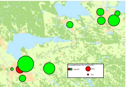
To achieve an ocular (graphic) impression of the DB/DBB difference, a two-step method has a merit. In Figure 3, our productivity is the model cost / real cost. The DB and all other procurement variables have been removed, but we have given all DBs one colour and shape and all DBBs another colour and shape. We now expected that DB would tend to “float” above the DBBs, reflecting a generally superior productivity, at least in some contract intervals.

Figure 3. How productivity depends on DB, DBB and contract size.

At least at first sight Figure 3 shows no obvious layering, with DB or DBB floating dominantly above the other. If looking more closely for intervals where this would be the case, there may be a tendency that when V (on the x-axis) reaches 200, the blue spots (DBB) tend to start to float above the red squares (DB) more generally, but future research is indeed appropriate to verify if this was a coincidence or a pattern.

Expert judgment or regression? Maybe future development will find a way to combine the advantages of regression-determined coefficients with those of expert judgments. On the other hand, when the number of observations increases, the model quality achieved by regression will probably gradually improve, reducing the need and advantages of the expert judgment method.

7.3 Logarithmating into percent

In Table 6, the second variable on the list is the design-build variable DB. All variables together explain 75 % of the cost variation (adjusted r2=0,754). The p-value for the model as a whole is very good (2.2 × 10-16). The coefficient for the design-build variable achieved with the one-step-method will correspond to its average influence on the contracts, expressed in Swedish kronor. But such an absolute value, 25.8 mkr in Table 6, is relevant only for this particular dataset. It is more generalizable to express the coefficient as a percentage of y.

The percentage can in this case be achieved by logarithmation of y (the actual contract cost) before the regression. The coefficient will then be the percentage change of y when each x variable increases by one unit, e.g. when the design-build increases from 0 to 1. (To find the mathematical proof for this, the reader is forwarded to statistical literature).

Thirteen variables plus DB and a constant delivered the highest adjusted r2, 0.4946 (and also the lowest p-value for F, 2.44×10-11, another possible criterion for optimum, which will not be further explained here, see statistical literature). In the final and optimal regression, the coefficient for DB was 0.1838 and the p-value 0.1152.

With more and less variables the coefficient went higher, up to 25 %. 18 % is therefore also the most cautious estimate among the candidates. The most cautious p-value would be 0.13 (Table 6).

Not captured in the cost data is the design costs of the DBB contracts. To the extent that they are included in the DBs and not in the DBBs, it can be argued that this should be compensated for. If assuming them to be 5 %, the calculation 1.18×0.95=1.12 leaves us with an estimate of a 12 % cost addition with DB and a p-value of approximately 0.4. The five percent is a very rough figure, an expert estimate, since a proper calculation would be considerable work with new data collection.

8 CONCLUSION

No established off-the-shelf methods to calculate productivity in infrastructure investments could be found in the initial literature scan, but a number of methods were developed and then used. We first calculated the annual productivity advance, which

turned out to be a net non-significant −3 % annual productivity decline, when

compensated with the general cost index NPI. Regarding the productivity difference between design-build DB and design-bid-build DBB, our most trustworthy and cautious analysis delivered a significant 18 % lower productivity for DB with a non-significant p-value of 0.13. If including compensation for an assumed 5 % design cost saving in DBs favour, the DB relative productivity is −12 %.

Our DB/DBB study suggests that the agency should start looking for other factors in the projects than changing them to design-build if they want to achieve higher productivity. The increased use of DB fits as an explanation of the annual decline in productivity. There may however also be other reasons.

It required substantial authority and power to motivate the agency to participate in the study and deliver data. This may explain why similar studies seem not to have been undertaken before, and why it may become difficult to copy or develop our study for new researchers. Future research is still encouraged to improve, complement, modify or replace our methods or reuse them as is with other variables or new data. The presented methods are possible to use also to analyse other procurement variables’ effects on productivity. There is today a lack of knowledge in this field and considerable costs at stake, possible to gain. An aim is to narrow the probability bell and reduce the confidence interval. This will sharpen the conclusions possible to make.

9 REFERENCES

Allen, S. G. (1985) Why Construction Industry Productivity is Declining. Review of Economics and Statistics, Vol. 517/4.

Ekonomistyrningsverket (2009) Handledning Resultatredovisning ESV 2009:29

Langford D. A., Kennedy P., Conlin J. and McKenzie N. (2003). Comparison of construction costs on motorway projects using measure and value and alternative

tendering initiative contractual arrangements. Construction Management and Economics, Vol 21/8, p 831–840.

Odhigu; F.O., Yahya; A., Rani, N. S. A.; Shaikh, J. M. (2012) Investigation into the impacts of procurement systems on the performance of construction projects in East Malaysia. International Journal of Productivity and Quality Management, Vol 9/1, p. 103–135

Pakkala, P. (2011). Improving Productivity Using Procurement Methods – an international comparison concerning roads. Swedish Public Enquiries SOU 2012:39 Part 2, chapter 3.7, p. 56.

Sandahl, R (1991) Resultatanalys. Riksrevisionsverket.

Sanvido V. E. and Konchar M. D. (1998) Project Delivery Systems: CM at Risk, Design-Build, and Design-Bid-Build. Research Report 133–11, Construction Industry Institute, Austin, Texas.

Stenbeck, T. (2007) Promoting Innovation in Transportation Infrastructure Maintenance, KTH Royal Institute of Technology, Stockholm, Sweden.

Vedung, E (2009). Utvärdering i politik och förvaltning.

Wherry, R. J. (1931). A New Formula for Predicting the Shrinkage of the Coefficient of Multiple Correlation. The Annals of Mathematical Statistics, Vol. 2, p. 440–457.

PRICING PRINCIPLES, EFFICIENCY CONCEPTS AND

INCENTIVE MODELS IN SWEDISH TRANSPORT

INFRASTRUCTURE POLICY

KTH Royal Institute of Technology Architecture and the Built Environment

SE-100 44 STOCKHOLM, Sweden

E-mail: bjorn.hasselgren@abe.kth.se

ABSTRACT

In this article the shift of the Swedish government’s policies for the financing through taxation, fees and prices paid for the use of roads and railroads from 1945 until the 2010s is discussed. It is argued that the shift from a full-cost coverage principle to a short term social marginal cost principle can be seen in the light of the controversy between a Coasean and a Pigovian perspective.

The Coasean perspective furthers an institutional view where organizations and dynamic development matters while the Pigovian perspective furthers a welfare economic equilibrium view where organizations are less focused. It is argued that the shift in policies coincided with less interest and focus on the organizational perspective and incentives for organizational efficiency, which can be seen in the public documents from the time.

The government seems to have been guided by a market failure stance since the 1970s which has motivated growing intervention, following a market-economy stance in the first 25 years after the nationalization of roads and railroads. A current opening in transport infrastructure policies with more room for alternative financing, user charges and fees might, even though also consistent with short term social marginal cost principles, signal a revival of a perspective more in line with the Coasean view.

1 INTRODUCTION

Transport infrastructure systems (here primarily roads and railroads) are expensive to build but generally relatively cheap to use for every single additional road vehicle or train. There have been discussions and diverging views in many countries around how to set an efficient framework for the pricing of the use of roads and railroads. Should e.g. the users pay the full cost or only the marginal cost connected to the use of roads and railroads? Is it appropriate for the government to cover a possible financing deficit with general tax revenues, if users pay only the marginal cost? Do such subsidies lead to good overall welfare based efficiency but less strong focus on organizational efficiency?

The Swedish government nationalized roads and railroads in the late 1930s and 1940s. One of the first issues it had to deal with following the nationalization during the second world-war was the financing of the coming investments in both roads and railroads and how to set the fees and taxes for the users of the infrastructure. Since the 1940s this discussion has been reopened on a number of times. In brief two different principles have been applied in this respect; a full cost coverage and a short term social marginal cost based view on taxation and pricing.

These two principles also reflect two different perspectives when it comes to the incentive structure that is applied for the management and financing of the organizations responsible for roads and railroads. According to one perspective a direct link between fees and taxes paid by users and spending by the government is the preferred model (also called ear-marking). According to another perspective other parties than the users, often the general tax payers, via government subsidies or cross-subsidies, should normally pay for major parts of the spending on roads and railroads.

A direct connection between the users and the provider of roads and railroads through the payment channel could generally be expected to give stronger incentives for organizational efficiency and user orientation than a system where funds are channeled through the government. Ear-marking by which tax income e.g. based on fuel taxes is allocated for road-purposes can in this respect be seen as a second best alternative to direct payments by the customers to the infrastructure organizations. At the same time it can be argued that an ear-marking system managed by the government will probably be just as inefficient as other financing mechanisms managed by the government, Wagner (1991).

The different perspectives for how to finance systems such as transport infrastructure were reflected in a series of articles by Ronald Coase in the 1940s and again in the 1970s (1946, 1947, and 1970). The reasoning in the articles seems surprisingly up to date after nearly 70 years. These articles are taken as a theoretical starting point for the following discussion and analysis.

Questions that are focused in this article are:

- Is it possible and relevant to interpret the government’s formation of pricing and taxation policies for the use of roads and railroads since the 1940s in terms of a shift from a full cost coverage principle to a short term social marginal cost principle for taxation and pricing?

- Have the different principles been discussed in terms of their impact on incentives for organizational efficiency in the transport infrastructure system? The article is based on studies of government committee reports, the government’s proposals to Parliament and the Parliament’s discussions and decisions in relation to the proposals. The studied reports and documents cover the time period from the 1930s up to the 2010s. Whether there is a transport infrastructure policy possible to study, as separate from the overall transport policy, can of course be discussed. It is rather obvious that the two policy areas are separated for roads while generally more closely connected for railroads, in specific until the separation of railroad services from railroad infrastructure in 1989. When it comes to the financing principles these have, however, been discussed as separate themes at a number of times, and are more easily separable from the overall policy discussions.

Two major economic theoretical perspectives and principles following from these are discussed in the article. On the one hand a neo-classical welfare theory based view. On the other hand an institutional or organizational view. Based on these two perspectives some central terms in the article are clarified here:

- Welfare economics – term used for an economic concept that aims for including all socially relevant aspects of the economic activity carried out, e.g. in relation to a road system, within a perspective where optimal allocation is sought for. In this perspective the operation of a transport infrastructure system is seen as an activity which should be dealt with in a wider public sector (political) perspective.

- Business economics – term used for an economic concept that aims for the analysis of (economic) organizations and their functioning when it comes to resource allocation, management and relations to the economy at large. The private corporation acting on a market is the natural starting point of analyses based on this perspective. The economizing behavior and practices of government agencies might also be analyzed according to these principles.

- In the discussion around these perspectives in the Swedish government reports etc. since the 1940s these two perspectives have been connected to a focus on “external” vs. “internal” perspectives on efficiency.

- Efficiency – from a welfare economic perspective has to do with the overall use of resources in a society in order to reach an optimal resource allocation. Efficiency as defined from a narrower business economic perspective has to do with the economizing activities in any business organization or government administration in order to make the best possible use of and allocation of available resources, primarily within the borders of the organization. Here, neo-classics is connected to the term “welfare based efficiency” or “external efficiency”, while an institutional perspective is connected to “organizational efficiency” or “internal efficiency”.

- Short term social marginal costs and short term marginal costs are terms used when analyzing how the flexible costs related to an economic system or to an organization can be measured, either from a welfare basis or from a business economics oriented approach. Policies for fees/pricing and taxation are often related to these concepts.

2 THEORETICAL APPROACHES TO PRICING

Over time successive investments in roads and railroads have led to the accumulation of a major asset-base which, from an economic point of view, can be treated as sunk costs. One reason is that even if the assets represent a considerable value they have few alternative uses. The cost of tearing down roads and railroads are also considerable.

The operation and maintenance of pavements, platforms, signal systems etc. is necessary for the use of roads and railroads. These operations represent (flexible) marginal costs. The use of roads and railroads induces additional wear and tear of the assets and thus related costs. Combined these costs are more or less equivalent to the short term marginal costs. If costs external to the operation of the system as such, e.g. congestion, noise and pollution, are included a short term social marginal cost construct is arrived at.

There is a sound economic basis for charging the users of the present road and railroad system only for these short term social marginal costs. If also the depreciation of the current systems, as well as investment costs for re-construction and new-construction of roads and railroads are considered, the cost basis is of course considerably much wider than what is represented by short term marginal cost concepts.

According to the principles developed in welfare economics through the late 19th and 20th centuries (Ruggles, 1949) by a number of scholars such as Marshall, Wicksell, Pigou, Hotelling and Lerner, only to mention some, consumers’ marginal utility when choosing different packages of goods and services, should be the basis for the analysis of, and decisions on, resource allocation in the economy. These theories are generally based on assumptions of perfect information, free entry and competition and rational

actors. The view on organizations is less well developed in this view and equilibrium on stable markets or in the entire economy more in focus.

Part of the same view is that decreasing-cost industries, such as roads and railroads could be expected to be organized as nationalized or regulated monopolies in order to avoid inefficiencies, such as monopoly pricing. In these cases (only) short term social marginal costs should, according to the same view, be charged for the use of the products or services. The unfinanced part of the costs, which are not covered for by short term marginal cost pricing based revenues should, according to the same line of reasoning, primarily be paid for by the government, funded with tax revenues.

Coase in his articles on the ‘Marginal Cost Controversy’ (1946, 1947) presented a different view on the preferable way of handling the pricing of services and goods in decreasing cost sectors. The original article was written in relief to the Hotelling-Lerner view, with its basis in marginal cost pricing and support of a system based on government subsidies. Coase presented four arguments in favor of an alternative pricing system based on multipart pricing, with separate payments to cover fixed and variable costs. With such a system the user would face the full cost of the resources that are used for the production of the good or service, which would confer a correct combined price signal.

Coase’s arguments against marginal cost pricing without full cost coverage are condensed into the following arguments:

- Marginal cost pricing would lead to “mal-distribution” of the production factors to different uses, since the full costs of these would not be obvious to the user. - Marginal cost pricing would lead to income distribution from non-users to users

and from tax payers to users.

- Marginal cost pricing if combined with tax subsidies would lead to “other harmful effects” as the economy is more heavily tax-burdened

- Marginal cost pricing would lead to a risk for over-consumption and lack of information on how to spend resources in the future, since price signals are distorted.

Coase’s discussion emphasizes the central role of the producing organization and its relation to users or customers. The organizational view can be traced back to Coase’s 1937-article ‘The Nature of the Firm’. This is a difference towards the neo-classical welfare view, with its limited focus on organizations. A parallel discussion is of course the market failure/government failure-divide where situation e.g. with less than perfect information or public choice inspired arguments have been used as support for either one of the two failure alternatives. See Medema (2009) for an historical overview of both this discussion and of Coase’s contribution.

While this discussion goes back at least to the 1930s Lindsey (2006), reflecting on the later development of economists’ views on road pricing up to the 2000s, notes (p 315) that the more institutional sentiment that Coase represents has not been the core element of economists’ handling of issues related to road pricing in general (as an area of academic interest close to the theme in this article). The view represented by Pigou has though, since the 1940s, largely been developed by a number of scholars such as Vickrey, Walters and Mohring. Pricing of road-use based on short term social marginal cost has been the basis for these later scholars’ writing. Small, Winston and Evans, among others, according to Lindsey, have shown that under some assumptions congestion and road damage charges can pay for the costs both for capacity and maintenance (p 312). This line of theorizing has also been possible to express in

mathematics and in graphical form, which has probably added to the strength of this view among economists, and also to its strong influence on the public discussion of the pricing issues.

The institutional view, which was exemplified by road and railroad-related themes in Coase’s 1940s articles have, according to Lindsey, not been widely developed with further applications in this sector of the economy. As an exception the writings of Gabriel Roth can be mentioned. Roth (2006) has edited one of the later works where a number of articles discuss the prospects and favors of a more privatized road provision, but has also published a number of books in this field since the 1960s. A similar approach is presented by Winston (2010). Winston suggests privatization experiments to be introduced as a means for addressing many of the problems of the US transportation system, such as lack of innovativeness, lack of resources and slow productivity growth. These two examples show that the institutional view is represented also by contemporary scholars, even if the welfare or neo-classical view is generally the stronger in discussions around transport infrastructure.

While Coase favored a system where roads and railroads were financed without government subsidies the more recent institutional studies mentioned above seem mostly to focus on an improvement and methodological refinement of the application of short term social marginal cost based financing models. By reducing cross-subsidies between different transport modes, and striving for setting prices and fees more in line with actual marginal costs (including e.g. congestion induced costs and external effects) an improved external or welfare based efficiency could be achieved than in many present systems.

This seems to be a view where a move from weaker to more powerful incentives is sought for, while not necessarily meeting Coase’s requirements, aiming for full cost coverage. Even if short term marginal cost pricing could be expected to raise sufficient resources to cover the full costs of roads in urban congested areas this would clearly not be the case in less populated areas. There would thus still be need for substantial tax-financing if these models are applied. This is of course something that is generally truer when it comes to railroads with its high infrastructure costs.

Coase

Pigou

The different perspectives are summarized in Figure 1 above. The x-axis shows different views on whether marginal cost or full cost coverage should be favored. On the y-axis the dichotomy between ear-marking (all government-collected revenues are directly allocated to the supplier) and the handling of revenues as general tax revenues is displayed. Coase’s model, placed in the upper left, combines full cost coverage with ear-marking (which is not explicitly stated by Coase but might be assumed from the general reasoning in the articles). The Pigovian welfare model is displayed in the lower right, combining marginal cost coverage with the treatment of revenues from taxes and fees as general tax income.

It could be argued that the Coasean view is more closely related to the first welfare theorem, aiming for an efficient allocation of resources through market processes, while the Pigovian view, also reflected by scholars like Wicksell, is closer related to the second welfare-theorem, where redistribution of resources through, possibly, political decision-making, is introduced. Blaug (2007) argues that the second theorem even “emerged out of a discussion of the principle of marginal cost pricing applied to public enterprises” such as natural monopolies.

Another interesting view also connected to the welfare theorems but closer to public choice theory, is represented by Wagner (2007), who argues that the traditional dichotomy between a “market square” and a “public square” where peoples’ life are spent, is a prerequisite for the development of welfare economics. In real life, however, Wagner argues, that it could be questioned whether this dichotomy really exists and further as regards whether there is only one, or more public squares, opening for a polycentric view. Wagner argues that a model where a more dynamic view on resource allocation could be a way forward in developing an alternative theoretical framework for discussion on “good management” and resource allocation. This view resembles some of the views also discussed by Coase favoring negotiations and the institutional framework in societies as important for achieving an efficient use of resources. There are clearly differing views on the proper basis for analysis and policy development in this field.

3 EXAMPLES FROM SWEDISH TRANSPORT

INFRASTRUCTURE POLICY

Three rather distinct time-periods can be observed when it comes to the government’s formation of pricing and financing policies for roads and railroads since the 1940s.

- The full cost coverage period 1945-1978 - The mixed pricing policies period 1979-1988 - The social marginal cost period 1989-

The following discussion is organized following these three periods.

3.1

The Full Cost Coverage Period

Following the nationalization of roads and railroads in Sweden by the late 1930s and early 1940s the government initiated the post war planning in the transport-sector. The first post- world-war two Transport Committee started its work in 1944. It presented its final report in 1947 (SOU 1947:85). The overriding principle for the management, planning and financing of transport infrastructure was defined to be to aim for broad

social welfare based efficiency, expressed as the highest possible output in relation to the resources used in the sector. In addition to this a principle of full cost responsibility for every single transport mode was proposed, echoing pre-war policies in this field.

Overall the Committee had a positive view on the value of free enterprise and competition as a basis for the development of a sound and efficient transport system, more than leaning towards centralized planning. Dynamism, technological development and competition were seen as superior aspects of a free market, compared to a government controlled development or “dirigisme”. This was a reasoning coming close to discussions raised in, at the time, current discussions raised by both Hayek (1944) and Schumpeter (1942), favoring entrepreneurial activity and with a critical view on planning and government intervention. The two representing different views on the possible future outcome of the balance between market and hierarchy; with Hayek favoring market solutions and Schumpeter projecting an inevitable “march into socialism”.

The 1944 Transport Committee´s proposals were, according to Sannerstedt (p 5, 1979), never followed by any explicit proposals by the government. When reading the government’s yearly budget bills for the years following the war-end it is obvious that the government instead focused on the need for tackling the overriding economic policy dilemma; a strong demand driven growth in consumption and imports and the necessity to balance this demand against the major needs for investments in most areas of the economy. To set up a separate road-management structure with an independent (from the government) set of accounts, as suggested by the 1944 Transport Committee in order to strengthen the business economic efficiency-incentives in the road administration, was never proposed by the government. This is presumably explained by the government’s willingness to preserve discretion in fiscal and budgetary matters.

The future of the general transport policy was however again in focus of the 1953 Transport Policy Committee, reporting in 1961 (SOU 1961:23). It presented a coherent plan for a sustained market oriented transport policy with focus on deregulation, where major remaining war-time regulations should be abolished. The basic strategy, with the focus on a business economic inspired framework and a cost responsibility principle, was also to be left unchanged.

The basis for (undefined but seemingly close to welfare) efficiency of the system was, according to the Committee, that the true (mainly direct financial) costs of the different transport modes were reflected in the prices and taxes that the transport users met. This was a direct link to the cost responsibility principle of the 1940s and 50s. This policy would enable choices in each single situation to be efficient as the costs of the services would be reflected against the willingness to pay for these services. It would also lead to a subsequent separation of transport flows to the different modes according to their relative strengths.

The Committee also discussed marginal cost-based pricing principles (at the time no specific definition of whether social or business economic efficiency was focused), which were said to be the correct pricing principle for the existing network at any given time. The Committee had, at the same time, the view that for new-construction the users should be charged the full costs of the projects. In a situation with a strong projected investment growth full-cost coverage would set a frame for the total investment volumes. There had been similar concerns over risks for over-investment, discussed in the government’s long term economic policy committees, set up by the ministry of finance. This risk, it was argued, could be met by this two-tier pricing policy.

The Transport Policy Committee’s work was commented on in the government’s proposal to Parliament in 1963 (1963:119). The government more or less endorsed the proposals of the Committee, as did the Parliament. This decision also summarizes and formalized the rather strong focus on the cost responsibility principle which had been dominating in the actual government policies since the mid-1940s.

3.2

The Mixed Pricing Policies Period

Through the 1960s there was a growing public discussion on the future development of the transport system as road traffic and private car ownership grew. One of the outcomes of the discussion was that there were political claims for the railroad system to be protected from further closures and questions were also raised whether the projected and prolonged strong growth of the number of motor vehicles was reasonable. The proper estimation of the social costs of the road-system, and the possible application of the economic principles also for the railroads was therefore one of the concerns in the late 1960s and early 1970s when discussing transport policy.

In order to answer to the public pressure for a revised transport policy as the critique against the perceived road-transport favoritism, and the cautions that the railroad-system was disadvantaged by the prevailing policies, the government decided to set up a new Committee, the 1972 Transport Policy Committee.

The government at this time aimed for a redirection of transport policy. The Committee expressed the main features of the new transport policy to be the wider welfare based (economic) goals. Within a framework of government ownership of transport infrastructure and welfare economic principles the transport services organized either as government agencies or private sector operations should, however, still be carried out with the overriding aim to achieve a more narrow organizational efficiency.

In a report from the Committee in 1978 (SOU 1978:31), focusing on the cost responsibility principles and fee-structures, the view that the cost responsibility perspective should be abolished for both railroads and roads was however advocated.

The Committee thus emphasized the wider welfare based economic perspective when it came to the management, financing and planning of transport infrastructure. The importance of organizational efficiency in the production of the services and the management of the government agencies in the area was only briefly discussed. Only one paragraph was included in the 1978-report (p 41) discussing the need for a focus on the internal efficiency of the agencies (and other organizations) in the transport sector. Little was said in this respect other than that “intense rationalization- and cost-reduction” should be the focus of the organizations and that “motivation” is important as the marginal cost principle would probably not give the best prerequisites for (internal) efficiency.

The government sent its proposal to Parliament in 1979 (1978/79:99). The 1963 goal for transport policy was proposed to be changed in line with the recommendations from the 1972 Transport Policy Committee. A new overriding goal for transport policy reflecting the shift to a welfare economic stance was proposed by the government.

Short term social marginal cost based pricing was seen as the preferable principle for future decisions on the prices and taxes in the area, and primarily when it came to the use of the existing network. At the same time the difficulties in applying these