Connecting casting simulation and FE software including local variation of physical properties. : Investigation on local material properties and microstructure in a grey iron cylinder head.

(1)

PAPER WITHIN Product Development and Materials Engineering AUTHORS: Fredrik Beckius & Robin Gustafsson

TUTOR:Jakob Olofsson JÖNKÖPING June 2016

- Investigation on local material properties and

microstructure in a grey iron cylinder head.

Connecting casting simulation and

FE software including local variation

(2)

Postadress: Besöksadress: Telefon: Box 1026 Gjuterigatan 5 036-10 10 00 (vx)

551 11 Jönköping

This exam work has been carried out at the School of Engineering at Jönköping

University in the subject area product development and materials engineering.

The work is a part of the two-year Master of Science programme. The authors

take full responsibility for opinions, conclusions and findings presented.

Examiner: Professor Anders Jarfors

Supervisor: Assistant Professor Jakob Olofsson

Scope: 30 credits

(3)

Abstract

1

Abstract

The automotive industry strive towards minimizing fuel consumption which is commonly done by reducing the weight for all ingoing components within a vehicle without jeopardizing the functionality. In the process of developing improved cast iron components, a research project CCSIM2 (Closing the Chain of SIMulation for cast components part 2) has been performed at Jönköping University, JU, in collaboration with the automotive industry in Sweden. The researchers at JU have been studying the topic of virtual and computational modeling of materials, trying to connect the microstructure of materials with the mechanical properties. When working with finite element analysis (FEA), material definitions are traditionally defined only by one material property for a whole component, assuming homogeneous properties. In order to predict the local mechanical behavior throughout a whole cast component and incorporate this into FEA for structural analysis a simulation strategy was formulated by J. Olofsson. In order to verify the software simulations, three truck engine cylinder heads were cast consecutively from the same melt with the intention to experimentally test the local material properties.

The thesis work presented aims towards gathering deeper knowledge about the casting process and the effect it has on the local mechanical and physical properties. Also to find an improved way to simulate the material behavior of a cast component before sending it to the manufacturing process in order to fit the industry’s demands for developing components at a lower cost and in shorter time. Investigations were made on the variations in mechanical as well as physical properties within the third cylinder head with the intent to validate the mechanical properties collected from the two previous examined cylinder heads. Also trying to connect the local microstructural variations of the physical properties throughout the cast component and implement these into a simulation methodology which combines casting simulation and finite element analyses. Additionally an investigation was performed regarding a modelling procedure for thermal conductivity of cast iron, based on microstructural parameters. The work roughly involved e.g. sample extraction, sample preparation, mechanical and physical property testing, microscope analysis using an optical microscope and image analysis software, casting simulations and FEA. All work was accomplished using Jönköping University’s workshop, computer software and lab equipment.

The result from the studies shows a small variation in the ultimate tensile strength (UTS) from samples extracted from the same locations in the three cylinder heads, standard deviations around 5 % of the mean value. Measurements also shows local variations of the mechanical properties with a difference of 22 % between the highest and lowest UTS-value within the component. Correlations can be found between the UTS-values and graphite particle area, amount of graphite particles per mm2_{and the ferret max (length of the graphite particles). Most}

of the physical properties were found to not have local variation, e.g. thermal expansion, density and specific heat. The thermal diffusivity and thereby also the thermal conductivity was found to have small variations within the studied component. A simulation methodology was successfully implement in order to connect the casting simulation and FEA. Investigations regarding the modelling procedure shows a superior prediction of the thermal conductivity when using only the 1 % largest graphite particles instead of the mean values of graphite particle area and length.

If considerations regarding the local variations of both the mechanical and the physical material properties are taken when designing cast components, combined with design optimization, truly optimized components can be achieved. This reduces the material usage which results in lower fuel consumption, leading to less emissions, for components used in the automotive industry. A benefit in an economic aspect but more importantly for the environment.

Keywords

Grey Iron, casting process simulation, Finite element analysis (FEA), local variations of mechanical and physical properties, material testing, modelling thermal conductivity

(4)

Acknowledgements

2

Acknowledgements

The authors of this thesis would like to take the opportunity to gratefully acknowledge the people that with their help and support made this thesis project possible.

Jakob Olofsson

Senior Lecturer

Materials and Manufacturing

For being our supportive project supervisor. Always being positive and excited about our work and guiding us during this master thesis project.

Aron Brehmer

Ph.D. Student For being our helpful assistant project supervisor. Assisting us in the practical part of this thesis project including optical microscope analysis and image analysis. Taishi Matsushita

Assistant Professor

Materials and Manufacturing

For his assistance and expertise instructing us how to operate all the physical property testing equipment.

Jörgen Bloom

Laboratory Engineer For his instructions how to operate the sample preparation equipment, as well as the tensile test machine.

Toni Bogdanoff

Research Assistant For being our go to guy during machine breakdowns and always helping us with a smile on his face. Esbjörn Ollas &

Peter Gunnarsson

Laboratory Technologists

For instructing us on how to use the machines in the work shop.

Kent Salomonsson

Associate Professor Machine Design

For his helpful assistance setting up the Finite Element– model.

A special thanks goes to the industrial partners in this research project, Volvo Group Trucks Operations in Skövde and Volvo Group Trucks Technology in Gothenburg for providing the three cast cylinder heads that have been studied in this project.

The authors would also like to express their sincere thanks to the Material and Manufacturing department at Jönköping University School of Engineering that have provided us with office space and all the free coffee needed for our brains to function in the late afternoons. We are also grateful to all of the people working at the department enlighten our days and especially for serving us the many delicious Friday-fikas.

(5)

Contents

3

1 Introduction ... 6

1.1 BACKGROUND ... 6

1.2 PURPOSE AND RESEARCH QUESTIONS ... 6

1.3 DELIMITATIONS ... 7 1.4 OUTLINE ... 7

2 Theoretical background ... 9

2.1 RESEARCH APPROACH ... 9 2.2 GREY IRON ... 10 Composition ... 10 Microstructure ... 10 2.3 MECHANICAL BEHAVIOR ... 14

Modelling of tensile deformation curve ... 14

2.4 PHYSICAL PROPERTIES ... 16 Thermal expansion ... 16 Density ... 17 Specific heat ... 17 Thermal conductivity ... 17 2.5 MATERIAL TESTING ... 21 Tensile testing ... 21 Dilatometer (DIL) ... 21 Density determination ... 22

Differential Scanning Calorimetry (DSC) ... 22

Laser Flash Apparatus (LFA) ... 23

3 Method and implementation ... 25

3.1 THE COMPONENT STUDIED ... 25

3.2 SAMPLE EXTRACTION ... 25

Mechanical property sample extraction ... 25

Physical property sample extraction ... 28

3.3 TESTING ... 30

Mechanical property testing ... 30

Physical property testing ... 31

(6)

Contents

4

Extracting samples from mechanical tested samples ... 32

Extracting samples from where the physical samples were taken ... 32

Embedding samples ... 33

Grinding & Polishing samples ... 34

Etching samples ... 35

3.5 MICROSTRUCTURE ANALYSIS ... 36

Optical microscope analysis ... 36

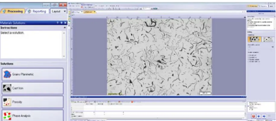
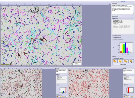
Image analysis ... 37

3.6 CONNECTING CASTING SIMULATION AND FE SOFTWARE ... 40

Design of simplified geometry ... 41

Setting up the FE-model ... 41

Casting simulation ... 42

Connecting experimental results to casting simulation results ... 43

Mapping the casting simulation results to the FE-mesh ... 43

FEA ... 43

4 Results & Analysis ... 44

4.1 MECHANICAL TEST RESULTS ... 44

Comparing the UTS-values between the three cylinder heads ...45

Microstructure analysis comparing six selected samples ... 49

4.2 PHYSICAL TEST RESULTS... 57

Dilatometer – thermal expansion ... 57

Density ... 58

DSC – Specific heat ... 60

LFA – Thermal diffusivity ... 61

Thermal conductivity ... 62

Microstructure analysis ... 64

4.3 COMPARING MODELLING- AND EXPERIMENTAL VALUES FOR THERMAL CONDUCTIVITY ... 68

4.4 FEA RESULTS ... 70

Experimental values ... 70

Extreme values ... 73

5 Discussion and conclusions ... 76

5.1 DISCUSSION OF METHOD ... 76

Sample extraction ... 76

Testing ... 76

Sample preparation ... 77

Connecting casting simulation with FE software ... 78

(7)

Contents

5

Mechanical test result ... 78

Physical test result ... 79

Modelling and experimental values of thermal conductivity ... 80

FEA results ... 80 5.3 CONCLUSIONS ... 80 5.4 FUTURE WORK ... 82

6 References ... 83

7 Search terms ... 86

8 Appendices ... 87

8.1 APPENDIX 1 ... 88 8.2 APPENDIX 2 ... 89 8.3 APPENDIX 3 ... 90

(8)

Introduction

6

1 Introduction

This master thesis investigates the local variation of mechanical and physical properties of a grey iron cylinder head. The local variation in properties is also connected to microstructural parameters of the material. Finally, it also connects the casting simulation of a component to finite element analysis (FEA) of its behavior during usage. The thesis covers the exam work within the two-year Master of Science programme Product Development and Materials Engineering at Jönköping University School of Engineering. The work has been part of a research project within the Materials and Manufacturing department at Jönköping University.

1.1 Background

A better understanding of the casting process and its effect on the local mechanical and physical properties can lead to better cast component with improved properties. A way to simulate the behavior of a cast component prior to manufacturing is in line with the industry’s strive for product development of improved components at lower cost and in shorter time. This can in the long run lead to more optimized designs of components and thus lower weight which, if used in the automotive industry for example, will lead to lower fuel consumption and thus lower emissions. A both economic and environmental benefit.

Jönköping University, JU, has a rich history of world leading research related to casting and the research is made in close collaboration with the industry. The research group Materials and Manufacturing at JU are performing research on the topic Virtual and computational modeling of materials where for example the connection between microstructure of materials and the mechanical properties are connected. This thesis work is a part of the research project CCSIM2 (Closing the Chain of SIMulation for cast components part 2) with the industrial partner Volvo Group Trucks Operations in Skövde and Volvo Group Trucks Technology in Gothenburg. J. Olofsson, in his doctoral thesis, formulated a simulation strategy to predict the local mechanical behavior throughout a whole cast component and also incorporate this into FEA simulations for structural analysis. The standard way of doing material definitions in FEA is to define only one material property for a whole component assuming homogeneous properties. However, as Olofsson emphasizes the complex casting process with e.g. varying thickness and thus varying solidification conditions leads to local variations of the material properties. The computer software developed by Olofsson creates material definitions for FEA which capture the local variations of the mechanical behavior. He found that the stress and strain distribution when including the local variations differed from the homogeneous material description. In the research done by Olofsson, cast aluminium and ductile iron components was investigated in order to demonstrate the simulation strategy's relevance. In order to try to verify the software simulations with physical testing of the mechanical properties, a truck engine's cylinder head has been investigated. Three cylinder heads were cast consecutively from the same melt. Two of them has already been tested with tensile tests from 30 different locations throughout the component. The third cylinder head has not yet been tested which is why it is in the scope of this thesis to test the last one in order to verify the variation of the mechanical properties. The microstructural variations have to a limited extend been investigated of the two previous cylinder heads. Sample preparations for microstructure analysis has been performed for a few selected sample locations throughout the component and also images from optical microscope analysis has been taken from those samples.

What has not yet been investigated is to perform a comprehensive analysis of the microstructure and relating it the local variations of the mechanical properties and also the physical properties, which has not been investigated at all. Connecting the local microstructural variations throughout a cast component to the physical properties and implementing this into a simulation methodology which combines casting simulation and FEA is, to the authors' knowledge, something that has never been done before.

1.2 Purpose and research questions

A grey iron cylinder head from an industrial casting is to be investigated of its variation of material properties within the component, both mechanical and physical properties. A connection between the variation of properties and the local microstructure of the material is

(9)

Introduction

7

also to be made as well as working out and describing a methodology how to connect casting simulation with FE software to include local variation of physical properties. The research questions sought to be answered in this thesis are:

 Will the local mechanical properties of cylinder head one and two be validated by the results from the third cylinder head?

 How are the mechanical properties varying within the studied component and can the variations be connected to the local microstructure of the material?

 How are the physical properties varying within the studied component and can the variations be connected to the local microstructure of the material and be predicted by a casting simulation?

 How can a casting simulation be connected to a FE software to include local variation of physical properties in FEA?

Also examined in this thesis is a modelling procedure for thermal conductivity of cast iron based on microstructural parameters. The aim is to compare modelled values to experimental values from the studied cast component.

1.3 Delimitations

An investigation of the local variation of material properties in a casted grey iron cylinder head is conducted. No other alloys or components are studied in this thesis. The FEA made are using only the physical properties of the material which is experimentally determined in this thesis. The mechanical property testing is limited to tensile testing in order to verify the result from two previously studied components from the same melt. The microstructural analysis of the mechanical test samples is performed on six selected samples from each of the three cylinder heads, not on all the tested samples. The microstructure analysis is limited to the graphite microstructure and identifying the phases of the matrix of the grey iron, not analyzing the local variation of the matrix in detail.

1.4 Outline

The thesis begins by providing the reader with the theoretical background needed to understand the work conducted. How the approach to the research has been made is described including a graphical representation of the research approach. The studied material, grey iron, is described including its microstructural features. The mechanical behavior and the physical properties of grey iron as well as ways to model the mechanical behavior and the thermal conductivity are discussed. General information about the testing equipment used to determine the material properties is also provided.

How the work is carried out and the methods used is described in detail including how and where all the samples for mechanical and physical property testing were made. The testing procedures with all the parameters used when testing is defined. How the samples were prepared for, and examined, in optical microscope is explained as well as how the graphite microstructure is quantified using image analysis. The methodology to connect casting simulation to a FE software using local material properties determined experimentally is then described. The set-up of a FEA of the component to compare using a homogenous material definition to local variations in the material based on casting condition is described.

The results from all the material testing, mechanical and physical, is then presented and analyzed. The mechanical properties are compared to the results from the two previous components studied from the same melt. Images of the graphite microstructure from the same positions in the three components are compared. The connection between microstructural parameters of the graphite and the mechanical properties is examined in order to identify correlations. The samples for physical testing are also examined to find connections between the experimental test results and graphite microstructure from three different solidification

(10)

Introduction

8

times. Models for thermal conductivity based on the graphite microstructure are then compared to the test results. Also the results from the FEA are presented and analyzed.

Lastly the methods used in this thesis as well as the results are discussed. Conclusions are then drawn and recommendations for future work is also provided.

(11)

Theoretical background

9

2 Theoretical

background

This chapter describes the theories found in the literature that covers this thesis’ topics. The research approach in the work is first presented followed by information about grey iron, the mechanical behavior of the material, the physical properties of it and common testing methods for determining the properties of the material studied in this thesis.

2.1 Research approach

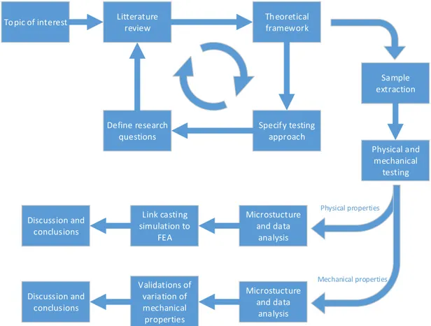
Since this thesis will consist of experimental research the approached used is positivism which traditionally is associated with deductive reasoning and linked with hypothesis testing and quantitative methods.[1] Figure 1 shows an illustration of the research approach used in this thesis. It is based on an illustration of the positivist research design described in the book Research methods for students, academics and professionals [2] and a modified version of that illustration in the dissertation by J. Olofsson [3]. In this thesis the creation of hypothesis is mainly replaced with forming of research questions and they are attempted to be answered within the frame of the thesis work.

Litterature review Theoretical framework Specify testing approach Define research questions Physical and mechanical testing Microstucture and data analysis Link casting simulation to FEA Discussion and conclusions Topic of interest Microstucture and data analysis Validations of variation of mechanical properties Discussion and conclusions Physical properties Mechanical properties Sample extraction

Figure 1. Illustration of the research approach used in this thesis.

The literature review contained reading previously published related research on the area of subject, e.g. J. Olofsson’s doctoral thesis and the reports from the two previous tests performed on the other cylinder heads [4, 5]. The literature also included other doctoral theses, scientific articles and books.

The knowledge from the literature review is the base of the theoretical framework this thesis is based on. The framework also contains knowledge about the various machines and testing equipment used during the thesis work, the information was found in reading material about the equipment and getting personal instructions on each machine by experienced personnel. A full list of the literature and other sources of information to this thesis can of course be found in the reference list in section 6 and the people giving instructions are credited in the acknowledgements.

(12)

10

2.2 Grey iron

Grey iron, also called flake/lamellar graphite iron (FGI) is one classification type used to distinguish the varying microstructures of cast irons. The classification names are primarily describing the shape, size, distribution and quantity of the graphite found inside the alloy. Cast irons are a class of alloys within the large family of ferrous metals and as for all the cast irons the main component is iron (Fe). In grey iron the alloying elements can be divided into three groups e.g. the major alloying elements, the minor alloying elements and the trace elements.[6]

Composition

The major alloying elements of cast irons are carbon (C) and silicon (Si), making grey iron a Fe-C-Si alloy.[6] The chemical composition of grey iron usually contain a carbon content in the range of 2.5 - 4.0 % and a silicon content around 1.0 - 3.0 %.

The minor alloying elements e.g. phosphorus (P), sulfur (S) and manganese (Mn) are also added to the melt.[7] Addition of phosphorus has been observed to reduce both the mechanical properties i.e. tensile strength of the grey iron, and the eutectic temperature. The later mentioned effect has shown to increase the fluidity of the melt.[8] Sulfur has normally been considered to be an undesirable element in grey iron not only due to its promotion of e.g. intermetallic carbides and an increased chill tendency which exhibits negative effects, but also due to its reaction with iron. The reaction between S and Fe produce the phase FeS, which has a low melting point and can in elevated temperatures adopt a brittle behavior. To avoid the undesirable outcome of the FeS phase manganese is added to the melt to tie up the sulfur and produce MnS. Addition of sulfur has also exhibited positive effects e.g. promoting nucleation of graphite and increase the strength of the material up to a certain level.[9]

The trace elements, which has concentrations lower than 0.01 %, can involve e.g. aluminium (Al), bismuth (Bi), calcium (Ca), lead (Pb), tellurium (Te), titanium (Ti), tin (Sn) or nitrogen (N), and can be present in the grey iron either intentionally or unintentionally. The trace elements can have an important influence on both the microstructure and the properties of the grey iron.[6]

Microstructure

The graphite microstructure in grey iron can be characterized in different ways. The composition and the solidification condition of grey iron gives rise to the different microstructures in the material.

Graphite characterization

The graphite in cast irons are generally categorized into three main morphologies, e.g. lamellar, compacted or nodular. The shape of the graphite is determined by the preferred growth direction of the graphite within the hexagonal crystallographic structure, as can be seen in Figure 2.[10]

Figure 2. The hexagonal crystallographic structure of graphite [11].

It has been shown that the preferred direction of growth for the lamellar graphite is along the a-axis, to the contrary of nodular shaped graphite that shows a preferred growth direction in a

(13)

11

radial manner along the c-axis. The compact graphite does not have one preferred growth direction and its growth mechanism seems more complex.[10]

In the flake/lamellar graphite iron, the graphite flakes can form in a variety of patterns and sizes. Both the pattern and the graphite flake size inside the grey iron are, according to the ASTM Internationals standard A247-10 [12], divided into two separate charts. One chart is identifying the pattern as either one of five types of patterns were each type has been assigned a classification letter going from A to E as seen in Figure 3. The other chart is identifying the graphite flake sizes and is subdivided into eight different length intervals as seen in Figure 4 and Figure 5.[12]

Figure 3. Displaying different distribution types of graphite flakes in grey iron according to the ASTM standard A247-10.[13]

Graphite flakes of type A has intermediate flake size and are defined as flakes randomly oriented inside the matrix.[14] Type A graphite is preferred for most applications but has demonstrated superior wear properties in comparison to the other types.[7]

Type B graphite is commonly described to have a rosette pattern where the flakes grows like clusters in the shape of rose petals. This distribution is typically observed when the cooling rate is fairly rapid such as in a component’s thinner sections or at the surface of the thicker parts.[7] Type C flake graphite is distinguished by its large flakes of typical kish graphite that is formed in hypereutectic grey irons. The large graphite flakes increase the thermal conductivity but decreases the Young’s modulus of the component.[7]

Graphite flakes of type D is characterized by small interdendritic flakes that displays a random orientation in the matrix. The small flakes of type D are commonly generated due to a rapid cooling rate or at locations in a component were the sections are thin. The small flakes promote good surface finish when machined but is often surrounded by a matrix of ferrite that can cause soft spots in the castings.[7]

Type E flake graphite is also characterized by small interdendritic flakes but exhibits an organized orientation inside the matrix. The matrix is commonly of pearlitic structure and can be compared with the wear properties of the type A graphite.[7]

(14)

12

Figure 4. The gradation of flake sizes in each size class, flakes measured in mm at a magnification of exactly 100 diameters.[12]

Figure 5. Graphite flake sizes in each size class as specified in ASTM A247-10.[15] The graphite flakes lengths are important when identifying the strength of a casting. For example, if the matrix structure is assumed to be identical in two type A castings, the casting displaying small shorter graphite flakes when observed in an optical microscope is the casting also demonstrating the highest strength.[14] This is because the shorter graphite flakes disrupt the matrix to a less significant extent than the longer or much larger flakes. The larger flakes however improves the properties of thermal conductivity and is desired in applications promoting good damping qualities.[15] Therefore when describing a casting microstructure both the pattern and the size of the graphite flakes are of significant value.[14]

Solidification of grey iron

In order to estimate the structure of an iron-carbon alloy such as grey iron, the simplified model of the binary iron-carbon phase diagram is not enough. The complexity of the phase relationships between the alloying elements requires a more accurate clarification method. One approach is by using the carbon equivalent value, CE. By adding the most important alloying elements in their weight percentages together with the percentage of carbon, the CE value can be derived. In equation (1) both the carbon and the silicon percentage is taken into account.[10]

% %

3 (1)

If the accuracy of equation (1) is still not fulfilling, an even more accurate approximation of the metal structure needs to be used. This is commonly done by adding the weight percentage of phosphorous to the equation as seen in equation (2).

% %

3 %

3 (2)

Equation (2) is the one that demonstrate most similarity to the equation used by Volvo. Volvo use a modified version that calculates the CE value of grey iron as shown in equation (3).

% %

4 %

(15)

13

The calculated CE value is used to categorize the melt of the grey iron into either a hypoeutectic, a eutectic or a hypereutectic grey iron. The eutectic grey iron normally has a CE value of 4.3 % whilst a hypoeutectic has a value below 4.3 % and a hypereutectic a value higher than 4.3 %. The three categories displays a distinct difference in microstructure when observed in an optical microscope as seen in Figure 6.[10]

Figure 6. Microstructure of unetched grey iron samples. (A) Hypoeutectic (<4.3% CE), (B) eutectic (4.3% CE), (C) hypereutectic (>4.3% CE).[16]

When observing the solidification sequences of the three categories, dissimilarities can be seen in the first phase that is precipitating as displayed in Figure 7.

When solidification occurs in a hypoeutectic melt the first phase to precipitate is austenitic dendrites. As the proeutectic phase will continue to grow the carbon level will increase in the rest of the melt until the melt reaches the eutectic temperature, TE. When TE is reached the

eutectic solidifications begins with eutectic growth from numerous nuclei points. The eutectic cells that has formed grows with almost spherical structure until they have consumed the remaining liquid. The proeutectic austenitic dendrites grows parallel to the eutectic austenite but is hard to distinguish without etching the samples.[7]

In a eutectic melt, solidification starts at a regular eutectic temperature, TE,without any prior

formation of proeutectic constituent. It makes the solidification rate the controlling factor. If there is enough undercooling during the solidification the TE can be lowered which can result

in a modification of the expected microstructure, e.g. go from a type A to E or form carbides.[7] When the hypereutectic melt solidifies, kish graphite is the first to precipitate and can be described as large, straight flakes or as thick, lumpy flakes that often are found at the surface of the melt due to their low density. When the temperature has been lowered to TE the remaining

liquid will continue to solidify with a eutectic structure.[7]

Figure 7. Schematic section of the eutectic region of the Fe–C equilibrium diagram.[16] The austenite phase will start to decompose with further decrease in temperature by precipitating the dissolved carbon. When reaching the eutectoid temperature this transformation is completed with the result that austenite generally has transformed to either perlite with graphite or ferrite with graphite. Ferrite with graphite is mostly found if the cooling rate is slow, if the ferrite has a high silicon content or a high CE value. The transformation to perlite structure is common if the cooling rate is relatively fast with a relatively low CE value.[7]

(16)

14

2.3 Mechanical behavior

The mechanical behavior of metallic materials can be determined by applying a uniaxial tension load resulting in a stress-strain curve as can be seen in Figure 8. Stress is defined as in equation (4).

(4) Where F is the force and A is the cross-sectional area. Strain is a unit less measure of the distortion which during tensile testing is the elongation. Engineering stress and strain, shown by the red curve (A) in Figure 8, are calculated using the initial cross-sectional area, A0, while

true stress and strain, shown by the blue curve (B) in Figure 8, are calculated using the current area, A.

Figure 8. Typical stress-strain curves for structural steel [17]. The red curve (A) shows the engineering stress-strain and the blue (B) show the true stress-strain curve.

The mechanical properties, e.g. Young’s modulus (E), yield strength and ultimate tensile strength, can be extracted from a stress-strain curve. Yield strength is the stress at which the material starts to plasticize. For some materials, such as many steels, the yield strength (YS) is determined by the stress value where the linear part of the stress-strain curve transcends to the non-linear plastic part, see point 2 in Figure 8. For many cast iron alloys including grey iron the yield stress at zero plastic strain is hard to identify. The yield stress is therefore often determined at 0.2% plastic strain (Rp0.2). Ultimate tensile strength (UTS), the highest point on an engineering stress-strain curve, point 1 in Figure 8, is the maximum stress the material can withstand before breaking.[3]

Modelling of tensile deformation curve

In cast irons the deformation behavior is primarily controlled by the graphite phase and the constituents in the matrix. By modifying the amount of graphite and its morphology, both the elastic and plastic deformation will be affected. The deformation of a grey iron alloy has been observed and documented when subjected to a tensile test. Four stages of deformation has been distinguished[18]:

 Purely elastic deformation of matrix.

 Plastic deformation of matrix at point of high stress.

 Recoverable strain due to the opening of the graphite cavities.  Permanent strain associated with the opening up of cavities.

(17)

15

Due to the linear behavior of the true stress (Pa) and the true strain (-) within the elastic region of a tensile test curve an approximation of the true elastic strain (-) can be made using Hooke’s law, in which E is the Young’s modulus. [10, 19]

(5) The true total strain is divided in to the true elastic strain and the true plastic strain .

(6) For grey iron, which does not present a distinct elastic region, the Young’s modulus is hard to determine. Figure 9 shows two ways of approximating the Young’s modulus, one is by determining the slope of a tangent at 0. A more common way is to use the secant method at 25 % of the ultimate tensile strength in which the slope of the secant determines the Young’s modulus. The yield strength (Rp0.2) is also hard to determine since it is closely connected to the modulus of elasticity.

Figure 9. Two different ways to determine the elastic modulus for grey iron, tangent modulus at no load and secant modulus and 25 % of the UTS.[7]

The stress values of the plastic region can also be approximated using a variety of suitable equations, e.g. Hollomon, Ludwigson, Ludwik, Swift and Voce. Two of the most commonly used equations are the Hollomon equation and the Ludwigson equation.[10, 20]

⋅ (7)

⋅ ∆ , ∆ (8)

The Hollomon equation is derived from a previously used approximation model known as the Ludwik model that also contained the stress constant .[21] In the Hollomon equation the relationship between stress and plastic strain is defined using the strain hardening exponent (-) and the strength coefficient (-).[19] The value of gives an indication of the material strength and the forces required to deform it. The exponent provides important information concerning two material properties, e.g. it signifies the strain hardening or work hardening characteristics of the material and it also works as an indicator for the materials stretch formability. A material with a high value of is preferred for processes which involves plastic deformation while a material with a low value is a good machinable material.[20] The value of the strain hardening exponent varies between 0 and 1 and describes if the material

(18)

16

acts perfectly plastic ( 0) or if it has a linear deformation hardening behavior ( 1).[19] For most metallic materials the value varies between o.1 and 0.5.[18]

The Hollomon equation assumes a linear relationship between the logarithms of the true stress and the true strain where the exponent is given by the slope.[10] The Ludwigson equation later added an exponential correction term, (∆), to the Hollomon equation as seen in Figure 10. The correction term was added to account for deviations at low strains containing the new parameters (lnPa) and (lnPa).[10, 19, 21]

(9)

Figure 10. A typical double logarithmic plot of the true stress and true plastic strain. Presenting the curves of Hollomon equation and Ludwigson equation with the correction

term at low strains.[20]

2.4 Physical properties

Cast irons, including grey iron, cannot be seen as homogenous when looking at the different physical, or thermal, properties. The amount of graphite affects the density and the specific heat while the size, shape and distribution of the graphite flakes highly affects the thermal conductivity. The matrix structure however is having a significant influence of the thermal expansion of grey iron.[7] These four physical properties are described in this section. Density and specific heat are mostly of interest in order to be able to determine the thermal conductivity, which together with thermal expansion are important properties of a cylinder head and similar cast components that are subjected to heat during its service. E.g. thermal stresses are developed across the cylinder head due to non-uniform expansion caused by temperature gradients within the component during usage. Low thermal expansion limits the thermal stress and high thermal conductivity reduce the temperature gradient.

Thermal expansion

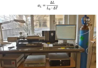
A material, most often, expands when heated. Thermal expansion is a measure of this tendency. It can be either the change in length or the volumetric change. The formulas for thermal expansion are[22, 23]: 1 ⋅ d (10) 1 d (11)

The coefficient αL, for linear, and αV, for volumetric, is the material property and the unit is 1/°C

or 1/K. The unit for αL is often expressed as µm/(m⋅°C) to get a more convenient number which

for most metals is between 5 and 25. The thermal expansion is not constant but varies with temperature. The coefficient is also referred to as CTE, coefficient of thermal expansion. For isotropic materials the volumetric thermal expansion coefficient is three times the linear expansion coefficient.

(19)

17

3 ∙ (12)

A low thermal expansion is desired in many applications, e.g. cylinder heads, where the dimensional tolerances needs to be kept at varying temperatures. For grey iron it is around 10 μm/(m·°C) at room temperature, but can rise up to 16.9 μm/(m·°C) at temperature up to 1070 °C.[7] Aluminium for comparison, which is both lighter and has higher thermal conductivity than grey iron, has a thermal expansion coefficient of around 23 which is why it is less common as a cylinder head material since it causes fretting and wear between the cylinder head and the cylinder block.[24] The matrix structure is what has the greatest impact on grey iron's thermal expansion. Ferritic and martensitic irons have slightly higher thermal expansion compared to pearlitic irons. The thermal expansion is commonly measured using a dilatometer.[7]

Result from experiments [25, 26] when measuring the thermal expansion for castings of the same melt in different solidification conditions, sand and insulation yielding solidification times of approximately 300 s and 1100 s respectively, shows no connection between solidification time and thermal expansion.

Density

Density is defined as the mass per unit volume and the formula for density is:

(13) Where n is the number of atoms in one unit cell, A is the atomic weight, VC is the volume of the

unit cell and NA is Avogadro’s number, which is 6.022·1023 atoms/mol.[27] The unit of density

is kg/m3_{, often also g/cm}3_{. According to Archimedes’ principle, the buoyance, the upward force,}

of an object submerged in a fluid is equal to the gravitational force on the displaced fluid. The following formula can then be used to determine the density of an object:

(14) Where ρ denotes density, m denotes mass and the subscripts o and f denotes object and fluid respectively. Since, as described in section 2.4.1, materials expand with increased temperature the volume and thus the density of a material decreases with an increase of temperature. Grey iron at room temperature has a density of around 6800-7400 kg/m3_{. The width of the span is}

due to the great difference in density of the microconstituents of grey iron. The matrix phases, e.g. ferrite, austenite, pearlite, cementite and martensite have densities around 7600-7900 kg/m3_{, while graphite has a density of only 2250 kg/m}3_.[7]

Specific heat

Heat capacity is a property which indicates a materials ability to absorb external heat. It represents the energy needed to rise the temperature of the material by one unit. Specific heat capacity, or often just specific heat, also includes the mass of the material, i.e. the energy needed to increase the temperature one unit per unit mass, which makes the formula for specific heat[22, 28]:

⋅ (15)

The unit for specific heat is therefore J/(kg⋅K). The subscript p denotes that it is maintained under constant external pressure. Specific heat is often measured by a Differential Scanning Calorimetry (DSC). Specific heat is highly temperature dependent, with higher values at higher temperatures. For grey iron at room temperature the value is around 565 J/(kg⋅K).[29] The specific heat is lower for graphite than for iron, meaning local areas of more graphite can have a slightly lower specific heat than area with less graphite, however the difference is small.

Thermal conductivity

A material’s ability to transfer heat is the definition of the property called thermal conductivity. It can be measured in several ways, either directly or, as has been done in this thesis, measure

(20)

18

the thermal diffusivity and then calculating the conductivity. Thermal diffusivity is a measure of a materials ability to spread, or diffuse, thermal energy. The thermal conductivity, λ (k is also often used), of a material is related to thermal diffusivity, α, by the materials specific heat, Cp

and density, ρ, by the formula[30]:

⋅ (16)

The unit of thermal conductivity is W/(m·K). The thermal diffusivity is, in this thesis, measured by laser flash analysis (LFA). The unit for thermal diffusivity is m2_{/s or often more conveniently}

mm2_{/s. In cast iron, including grey iron, several factors influence the thermal conductivity, e.g.}

graphite morphology, temperature, microstructure and alloying addition. The graphite’s shape has the most important influence where flakes of graphite have higher thermal conductivity than spheroidal or compacted shapes of graphite, as illustrated by Figure 11.[31] This means that grey iron, which is composed of graphite flakes, has higher thermal conductivity compared to other types of cast iron. The microconstituents of the material have different values of thermal conductivity, ferrite around 70-80 W/(m·K), pearlite around 50 W/(m·K) and cementite only around 7 W/(m·K). Graphite along the c-axis, see Figure 2, has thermal conductivity of around 80-85 W/(m·K) while for graphite along the basal plane, the a-axis, the thermal conductivity can be as high as 285-425 W/(m·K).[7]

Figure 11. Illustration of thermal transport in steel, nodular cast iron and lamellar graphite iron.[32]

As concluded in [33] structures with straighter and less branched graphite have higher thermal conductivity but the difference decrease at higher temperatures. Also, if cementite is present in the material the thermal conduction is reduced at all temperatures.

Modelling thermal conductivity

Grey iron, as all cast irons, can be seen as a composite material with several phases with different thermal conductivities. The total thermal conductivity of a phase is the sum of the contribution from heat carried by electrons and phonons, which comes from lattice vibrations.[34, 35]

(17) The thermal conductivity of cast irons can be estimated by knowing the thermal conductivity and the volume fractions of each microconstituents as well as the aspect ratio, also known as the shape factor of the graphite particles, ε [25]. The graphite particles are modelled as ellipsoidal discs with semi-axes of length c and a in the basal planes in the graphite so the shape factor is also referred to as c/a [36]. The aspect ratio can be determined by metallographic observations. First Löhe’s parameter, η, needs to be calculated [25, 36].

∙

(21)

19

Where lmax is the principal intersectional length of the graphite particles, called Feret max later

in the thesis, and A is the sectional area of it. Both chosen in an arbitrary cross-sectional metallographic plane. Löhe’s parameter can be referred to as the inverse of roundness. Roundness, or roundness shape factor (RSF), is defined as:

4 ∙

∙ (19)

Where A, Am and lmax or lm is defined as shown in Figure 12.

Figure 12. Illustration of the parameter used to calculate Löhe's parameter and roundness.[37]

Having Löhe’s parameter, η, the aspect ratio, c/a or ε, can be calculated by [36]

2 / 3 ∙ / ∙ 2 1 arccos / / ∙ 1 / (20) This is mostly used for calculation of the aspect ratio in CGI, for FGI the aspect ratio can be assumed to be 0.05 [34, 38].The effective thermal conductivity, λ*_{, of a grey iron alloy can be}

calculated as: [34] ∗ ∗ 1 3∙ ∙ ∗∙ , ∗ ∗ , ∗ 2 ∙ , ∗ ∗ , ∗ 3 ∙ ∙ ∗_∙ ∗ 2 ∙ ∗ (21)

In equation (21) the following two expressions are also needed:

∙ 2 2 ∙ ∙ 1 / _{∙ arccos} ₍₂₂₎

1 2 ∙ (23)

The subscripts α, β and γ represents the different phases, graphite, pearlite and alloyed ferrite respectively. The γ-phase is modelled as spheroids, the α-phase as ellipsoidal discs surrounded by a matrix of β-phase [25]. The volume fractions of the phases are denoted f. The graphite, α-phase, is significantly anisotropic and the subscript z represents the direction perpendicular to the basal plane, c-axis, while x represents the direction parallel to the basal plane, a-axis, λα,x λα,y>>λα,z. The alloyed ferrite is assumed isotropic while the pearlite is anisotropic with

λ∥ λβ,x λβ,y λβ,z λ and λ*β is the overall thermal conductivity of the pearlite matrix. The

thermal conductivity of the pearlite matrix is calculated as:

λ∗ 1

(22)

20

λ∥ ∙ λ ∙ λ (25)

λ

λ λ (26)

The thermal conductivity of each of the microconstituents in grey iron are listed in Table 1. Table 1. Thermal conductivity of the microconstituents in cast irons [34].

Microconstituents λ [W/m∙K] Alloyed ferrite (2wt% Ni, 1.5wt% Si) 30 Cementite 8 Graphite, λ∥ (a‐axis) 500 Graphite, λ (c‐axis) 10 Lamellar alloyed pearlite, λ∥ 27.3 Lamellar alloyed pearlite, λ 22.5

This model of the thermal conductivity is only valid at around room temperature and does not take into account the large influence the temperature has on the thermal conductivity of cast iron. Also, as concluded by Holmgren [25] this modelling procedure is quite accurate for compacted graphite iron and grey iron with undercooled graphite but it underestimatesthe thermal conductivity of grey iron with type A lamellar graphite, as seen in Figure 13. This might be explained by the fact that the graphite morphology and the aspect ratio is determined by sectioning the graphite particle in a 2D-plane.

Figure 13. Measured vs. modelled values for thermal conductivity for LGI=grey iron and CGI=compact graphite iron at room temperature.[25] The model underestimates the values

for grey iron with type A lamellar graphite, the values within the dashed circle. In a more recent paper by Holmgren [38] the thermal conductivity of graphite along the basal plane was determined inversely using equation (21) together with experimentally determined values for the thermal conductivity of the pearlite matrix [39], as can be seen in the left graph in Figure 14 and using an aspect ratio of 0.05. The effective thermal conductivity was established experimentally for a FGI with a solidification time of around 200 s. The calculated thermal conductivities of the graphite at different temperatures can be seen in the right graph in Figure 14.

(23)

21

Figure 14. Left graph showing experimentally determined thermal conductivities of different matrices. Right graph shows the calculated thermal conductivity of graphite along the basal

plane. [38]

2.5 Material testing

This section describes the different testing procedures used to measure the material properties described in section 2.3 and 2.4.

Tensile testing

Tensile testing, using a tensile test testing machine like the one seen in Figure 15, is one of the most common way to determine a material’s mechanical behavior. The tensile test specimen, with typically a circular cross section, are gripped in the testing machine by their large end section and an increasing tensile load is applied.[40] The ISO standard for tensile tests is ISO 6892-1.[41] A laser extensometer is used to measure the strain while the test is performed at a constant cross-head speed. The result is commonly in the form a table of the force applied and the actual cross section area for that force. Form that, a true stress-strain curve as described in section 2.3 can be compiled from which the mechanical properties, e.g. UTS, can be determined.

Figure 15. A Zwick/Roell Z100 tensile testing machine used to perform tensile tests. The displacement is measured using a green laser extensometer.

Dilatometer (DIL)

To measure thermal expansion of a material a push-rod dilatometer, like the one in Figure 16, is commonly used. First a small cylindrical shaped standard sample is placed in a furnace with a controlled atmosphere, often helium, and heated to a pre-determined temperature. Then the same procedure is made for the sample of the material to be tested. The change in length of the sample, which is caused by the thermal expansion of the material, is transmitted by a push-rod to a displacement gauge. Both the change in length, ΔL, and the change in temperature, ΔT, is

(24)

22

measured throughout the test. The thermal expansion coefficient, explained in section 2.4.1 can then be calculated using equation (27).[42]

∆

∆ (27)

Figure 16. A Netzsch DIL 402C push-rod dilatometer used to measure thermal expansion.

Density determination

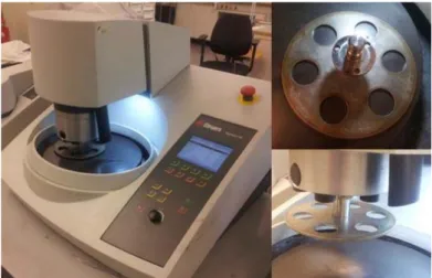
Archimedes’ principle can be used to measure the density of a material at room temperature, the principle is described in section 2.4.1. A sample of the material to be tested is weighed using an analytical balance together with a set for density determination, like the one seen in Figure 17. The sample is weighted first in the air and then submerged in water and weighted again. The analytical balancer then calculates the density of the material, using equation (14), and displays it. The density at any given temperature, ρ T , can be calculated using the density of the material at room temperature, RT, and the thermal expansion coefficient, αL at that temperature.[43]

1 3 ∙ ∙ ∆ (28)

Figure 17. An analytical balance used to determine density by weighing a sample first in air (left picture) and then in water (right picture).

Differential Scanning Calorimetry (DSC)

Differential Scanning Calorimetry (DSC), using a machine like the one seen in Figure 19, is a popular method to determine the specific heat of a material. It uses a single heating chamber to heat up two crucibles in a controlled atmosphere, often argon. The measurement must be run three times under equal conditions. First with two empty crucibles to get a baseline, then with one empty crucible and one with a standard reference sample. The third measurement is run with one empty crucible and one crucible with the sample of the material to test. The heat flow differences of the standard sample and the material sample to the baseline is then determined, defined as H as seen in Figure 18. The heat flow differences, H, the known specific heat, Cp, of

(25)

23

the standard and the two masses can then be used to calculate the specific heat of the sample material [44]:

∙ ∙

∙ (29)

Figure 18. DSC diagram showing heat flow differences.[44]

Figure 19. A DSC machine, Netzsch DSC 404 C, used to determine the specific heat.

Laser Flash Apparatus (LFA)

As mentioned in section 2.4.4 the thermal diffusivity is often measured when the thermal conductivity is sought. The laser flash method, using a laser flash apparatus like the one seen in Figure 20, is a standard way of measuring thermal diffusivity of a material. A disc shaped sample of the material, which must be opaque against laser, is heated at one end by a laser pulse inside a heating chamber with a controlled atmosphere, often argon. The heat from the laser is transported through the sample and the change in temperature on the side opposite to the laser pulse is monitored. The thermal diffusivity can then be calculated by the half time method:

0.1388 ∙

/ (30)

Where L is the thickness of the sample and t1/2 is the time it takes for the rear surface to reach

half of the maximum temperature. The unit of thermal diffusivity is m2_{/s. This formula is true}

if the system is adiabatic without radiation and if the material is homogeneous. Although there are models that corrects for the influence of heat losses and inhomogeneity.[45]

(26)

24

Figure 20. A laser flash apparatus, Netzsch LFA 427, used to determine the thermal diffusivity.

(27)

Method and implementation

25

3 Method and implementation

This thesis consists of a substantial amount of practical work, extracting material samples which were then tested to measure the material properties at different locations throughout the component studied. The material was also studied in optical microscope and the graphite morphology was quantified using image analysis. At the end of this chapter follows a description of a methodology worked out to connect casting simulations FEA using the experimentally measured local physical properties.

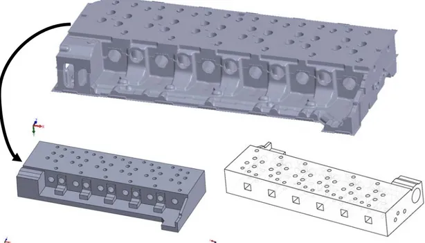
3.1 The component studied

The component studied in this thesis is a CH11 cylinder head from a Volvo truck diesel engine, weighing in at around 220 kg. It is cast in grey iron with the material composition as stated in Table 2. A cylinder head is a component which is bolted on top of the cylinder block of an engine and it is housing the valves for the inlet air and the exhaust gas, the fuel injector and cooling channels. The cylinder head is subjected to high temperatures during the combustions but also fluctuating temperatures and pressures.[24] A key aspect for the material in a cylinder head is that it must transport away the generated heat efficiently to limit thermal fatigue, i.e. have high thermal conductivity, while also maintaining the correct dimensions i.e. have low thermal expansion. The thermally induced stresses are also reduced by low thermal expansion, small thermal gradients and low stiffness of the material. The findings in this research is not limited to cylinder heads but could also be of interest in other components where the physical properties are of great interest, e.g. brake discs, cylinder blocks and furnaces.[32]

Table 2. Chemicalcomposition of the cylinder head.[5] Cekv is the carbon equivalent

calculated using equation (3).

C Si Mn P S Cr Ni Mo Cu Sn Ti V Cekv

3.11 1.88 0.49 0.05 0.09 0.14 0.06 0.19 0.83 0.051 0.010 0.017 3.61

3.2 Sample extraction

Material samples for testing were extracted at different locations throughout the cylinder head. How and where samples were taken and why they were taken at those locations are described in this section.

Mechanical property sample extraction

In total 30 tensile test specimens were extracted from the third cylinder head from six different locations in five of the six cylinders. No samples were taken from cylinder one due to its deviating geometry. The samples for mechanical testing were taken at locations according to an extraction plan from a previous work by T. Svensson and G. Stark [5], as seen in Figure 21, used for the first cylinder head. This plan was also followed in another previous work by M. Li [4] when studying the second cylinder head. This plan was followed in order to be able to validate the results of the mechanical testing from previous work.

(28)

26

The working steps when extracting the test specimens were as followed:  Removing excess material to fit the cylinder head into the bandsaw.  Cut the cylinder head into sections, one for each cylinder.

 Divide each cylinder section into an A-part and a B-part.  Extract rectangular cuboids of test specimens.

 Lathe the test specimens into cylindrical bars.  CNC-lathing into final tensile test bar shape.

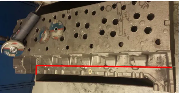
The tensile test specimens were machined to the correct size according to Volvo standard STD 1014,213 and the designation used is the 7C35.[46] The sample extraction was started by removing a large section, section zero, of excess material by angle grinding as marked by the red line in Figure 22. This was because the large 220 kg heavy cylinder head exceeded the maximum width of the vise of the bandsaw for metal cutting.

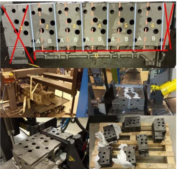
Figure 22. Section zero of excess material was cut off by an angle grinder at the red line. The cylinder head was then cut into six sections, one for each cylinders seen in Figure 23. Each cylinder section was cut into an A-part and a B-part.

(29)

27

Figure 23. Sectioning of the cylinder head using the bandsaw Bomar Proline 320.280 H. From each of the five cylinder sections four specimens were extracted from part A and two from part B making a total of 30 specimens. The rectangular cuboid shaped specimens, roughly 20x20 mm in cross section and a minimum length of 110 mm, were then roughly lathed down to cylindrical bars with diameters of 12 mm, as seen in Figure 24. The rotational speed of the lathe was set to 840 rpm and the feeding speed was set to 0.14 mm/revolution. To be able to get the full length of the tensile bars they had to be flipped around and lathed on the full length. The shape of the final tensile test bars were made according to the Volvo standard [46] with the help of a CNC-lathing machine. The top and bottom end still with the diameter of 12 mm with a 50 mm long necking with diameter 7 mm. The transit radius between the necking and the two edges was set to 5 mm as seen in Figure 24.

(30)

28

Figure 24. The tensile test bars were cut into rectangular cuboids which were then lathed to cylinders and given its final shape with the necking in a CNC-lathe machine.

To be able to keep track of all the 30 final shaped tensile bars, names were given to them based on:

 cylinder section number, (2-6)  part A or B

 specimen placement number

For example, specimen named 6B2 explains that it is extracted from cylinder 6, part B with the placement number 2. The location of all samples in the cylinder head can be seen in

Figure 27.

Physical property sample extraction

Samples were also needed for the physical property tests, dilatometer test to measure thermal expansion, differential scanning calorimetry testing to determine the specific heat and laser flash apparatus testing to measure thermal diffusivity. All these test procedures have been described in section 2.5. The purpose of the physical testing was to test the material’s thermal properties at different locations, solidifying at different rates, in the component. It was decided to test at three different solidification times; fast, intermediate and slow, and with a sample size of three for each solidification condition making a total of nine physical test locations. These locations were determined by studying images from casting simulation performed in MAGMA[47] of the cylinder head showing the solidification times in sections throughout the whole component, see Figure 25. The three different solidification times were chosen to be:

 Fast solidification – around 200 seconds.

 Intermediate solidification – around 600-700 seconds.  Slow solidification – around 1700-1800 seconds.

The three samples from the intermediate solidification were taken at the surface of the cylinder head which is in direct contact with the cylinder block, which is the source of the heat. The physical properties of the material at this location were of great interest for the manufacturer, Volvo. The three samples from the slow solidification was taken from the center of the component. These six samples, from slow and intermediate solidification, were taken from cylinder section 3, 4 and 5 and after the mechanical sample extraction was finalized it was clear that the best decision was to take the physical test samples from part B which still had a lot of material to take samples from. The three samples from the fast solidification were taken next to each other from the thin section named “0” in Figure 23. The physical test samples were

(31)

29

named in accordance with the naming of the mechanical test samples only adding an F, representing physical, at the end. The location of the physical samples can be seen in Figure 25.

Figure 25. Solidification time of the cylinder head from a casting simulation made by Volvo and arrows showing the locations of the physical test samples.

A rectangular cuboid piece was cut out for each of the six physical test samples and they were then lathed to their final dimensions. The sample dimensions, in accordance to the test equipment’s guidelines, for the three tests were as follows:

 DIL – cylindrical rod with 6 mm in diameter 12 mm in length  DSC – cylindrical disc with diameter 4 mm and 1 mm in thickness  LFA – cylindrical disc with diameter 12.5 mm and 4.375 mm in thickness

The different samples can be seen in Figure 26. The samples for DIL and LFA were cut out from the lathed piece in the lathing machine, leaving a small stub that was then grinded off, as seen in Figure 26. The sample for the DSC were not taken at different locations due to the reason that the specific heat of the material is independent of the casting conditions which means that it will not wary within the component. They were instead all taken from one single lathed rod and cut out using a low speed saw, as seen in Figure 26.

Figure 26. The cutting in the lathe left a small knob that had to be grinded off. Slow speed saw for DSC samples. All different test samples.

All the samples extracted, both for mechanical and physical property testing, are shown in Figure 27, they are:

 Samples for mechanical testing: o A1 – Turquois o A2 – Grey o A3 – Green o A4 – Orange o B1 – Black o B2 – Purple

(32)

30  Samples for physical testing:

o 1F – Yellow o 2F – Red o 0F – Blue

Figure 27. Locations of the test specimens. The long cylindrical bars represent the locations for mechanical testing and the short cylindrical bars represents the samples for physical

testing.

3.3 Testing

The material property testing of the cylinder head consisted of the testing procedures introduced in section 2.5. The testing was both of mechanical and physical properties.

Mechanical property testing

The mechanical property testing in this thesis consisted of tensile testing since it was used in test the two previous cylinder heads.

Tensile testing

The tensile test was performed at room temperature at JTH test lab using the Zwick/Roell Z100 tensile testing equipment which has a load capacity of 100 kN. The strain elongation on each tensile bar was measured with a laser extensometer. The tensile testing was executed to be able to collect the mechanical properties at various locations of the cylinder head. The proceeding steps were roughly as follows:

 Measuring the tensile bars

 Configure the software parameters  Execute the tensile tests

 Collect the data given

The software used when performing the tensile tests needed the input value of the minimum diameter of the necking section of each tensile bar. The measurements were taken in three different areas of the 50 mm necking section, at the bottom area, in the middle and at the top area as could be seen in Figure 28. This was done in order to investigate if the fracture occurred where the tensile bars had the minimum diameter.

(33)

31

Figure 28. The tensile test bars were measured at three locations on the necking, at the top, the middle and at the bottom.

All parameter settings were then configured into the software to fit the settings from the previously projects performed by Stark & Gustavsson [5] and M.Li [4]. The grip pressure of the tensile bar holders was set to 200 bar to make sure that the tensile bar did not slip when pulled as seen in Figure 15. The gauge length distance of the laser extensometer was set according to the Volvo standard [46] getting readings with a distance of 35 mm apart. The crosshead rate was set to a constant speed of 0.5 mm/min with a preload of 200 N.

One of the samples was destroyed while performing the tensile test and therefore the data from sample 3A4 is missing. After each test the data was collected from the stress-strain curve provided from the software.

Physical property testing

Four different tests, described in section 2.5, were performed to measure the material’s physical properties.

Dilatometer testing

The thermal expansion of the samples was measured by a Netzsch DIL 402C push-rod dilatometer, as seen in Figure 16. Due to technical problems with the machine, only six samples were measured, the three from slow solidification and the three from intermediate solidification. This is discussed further in section 5.1.2. The heating chamber was emptied of its air, creating a vacuum, and then filled with Helium gas. This process was done three times to ensure a high enough fraction of Helium in the atmosphere in the heating chamber. The testing was performed at two different occasions, each time doing a standard sample test, with a 12 mm long polycrystalline Al2O3 rod, before testing the material samples. At the first occasion samples

5B2F, 4B2F and 3B2F was tested and then the other three were tested. The testing was run from room temperature up to 500°C with a heating rate of 10 K/min. All samples were measured before testing and their lengths can be found in Appendix 1.

Density testing

The density was measured of the six samples made for the LFA testing before the LFA tests. The density was determined using the method described in section 2.5.2 using a KERN ABJ analytical balance as seen in Figure 17.

DSC testing

The specific heat measurement was performed using a Netzsch DSC 404 C as seen in Figure 19. The measurements were made from room temperature up to 500 degrees with a heating rate of 10 K/min. The atmosphere in the heating chamber was composed of Argon gas with a constant gas flow of 85 ml/min after the atmosphere was set to vacuum three times, just like for the dilatometer. In the first run, the correction run, the two crucibles were empty. In the second run, the standard run, one crucible was empty and one contained a standard sample of synthetic sapphire, α-Al2O3. Then the three samples were run successively with one empty crucible and

one crucible with a sample. The sample were first weighted and their mass was entered into the DSC computer program. Their mass can be found in Appendix 2.