Independent project/Degree project/Master’s thesis · 30 hec ·
Advanced level Programme/education · Environmental Economics and Management · Degree thesis No 1197 · ISSN 1401-4084
2019
Analysis of production risk and technical
efficiency amongst smallholder livestock
farmers in Botswana
iiii
Analysis of production risk and technical efficiency amongst smallholder livestock farmers in Botswana
Boitshepo Chube
Supervisor: Yves Surry
Swedish University of Agricultural Sciences Department of Economics
Examiner: Rob Hart
Swedish University of Agricultural Department of Economics Sciences
Credits: 30 hec Level: A2E
Course title: Degree Project in Economics Course code: EX0537
Programme/Education: Environmental Economics and Management,
Master’s Programme
Faculty: Faculty of Natural Resources and Agricultural Sciences Course coordinating department: Department of Economics Place of publication: Uppsala
Year of publication: 2019
Name of Series: Degree project/SLU, Department of Economics No: 1197
ISSN 1401-4084
Online publication: https://stud.epsilon.slu.se
Key words: Production risk, technical inefficiency, smallholder farmers,
Acknowledgements
I would like to thank the Swedish government for granting me the Swedish Institute Study Scholarship. This thesis would have not been possible without financial help from Swedish Research Council, Grant no. 348-2014-4293.They sponsored my field trip to Botswana to conduct data collection and analysis. I am also grateful for The Smallholder Livestock Competitiveness Project” funded by the Australian Centre for International Agricultural Research (ACIAR) and implemented by the International Livestock Research Institute (ILRI) in partnership with the Botswana Ministry of Agriculture’s Department of Agricultural Research for allowing me to use their data in this study.
Special thanks go to my supervisor Professor Yves Surry for his diverse contribution, patience and guidance towards the completion of this study. I also would like to thank Dr Sirak Bahta of ILRI and Dr Franklin Amuakwa-Mensah who has been of great help in many aspects throughout my study.
I am thankful for the Ministry of Environment, Natural Resources Conservation and Tourism for allowing me to pursue this programme by giving me study leave. I thank my family and friends for their continuous support while I was studying. Above all else I am indebted to God for sustaining me throughout my stay and study in Sweden and seeing this work unto completion.
iv
Abstract
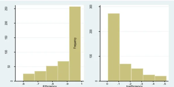
Achieving full efficiency is what every farmer desires to attain however due to constraints that they are faced with this is usually not possible. This study uses cross-section data to identify the shocks or risks that Botswana’s smallholder livestock producers are exposed to as well as their coping strategies. At the outset a sample of 540 observations which includes large and small beef producers are used but the econometric model estimated in the thesis is only limited to small beef producers. Furthermore, the study seeks factors that determine technical efficiency amongst small beef producers. The preliminary estimation of the Just-Pope production function did not lead to interpretable econometric results and for this reason, a change had to be made in the adopted empirical model. An alternative stochastic production model has been implemented empirically and estimated using a maximum likelihood (ML) estimation approach. The empirical results show that herd size and off-farm income reduce technical efficiency, an increase rainfall and household size were found to increase inefficiency. Moreover, production risk increases with an increase in maximum temperature but reduces with an increase in rainfall. The mean technical efficiency for the study area is 0.837.
Abbreviations
ACIAR Australian Centre for International Agricultural Research BMC Botswana Meat Commission
BWP Botswana Pula
DEA Data envelope analysis EU European Union
EPA Economic Partnership Agreements FMD Foot and Mouth Disease
ILRI International Livestock Research Institute ML Maximum Likelihood
SADC Southern African Development Cooperation SFA Stochastic Frontier Analysis
Table of Contents Acknowledgements ... i Abstract ... ii Abbreviations ... iii Table of Contents ... iv List of figures ... vi List of tables ... vi 1. Introduction ... - 1 -
1.1 Livestock situation in Botswana ... - 1 -
1.2 Research problem ... - 2 -
1.4 Objectives of the study ... - 4 -
1.5 Organization of the study ... - 5 -
2. Literature review ... - 6 -
2.1 Risk in Agriculture ... - 6 -
2.2 Measures of technical efficiency ... - 9 -
2.3 Review of empirical applications of the stochastic frontier analysis ... - 12 -
2.3.1 Existing empirical studies on technical efficiency in Southern Africa .... - 12 -
2.3.2 Studies from Botswana on technical efficiency ... - 13 -
2.3.3 Studies on production risk and technical efficiency ... - 14 -
3. Methodology ... - 17 -
3.1 Just-Pope production function ... - 17 -
3.1.1 Model specification ... - 17 -
3.2. Stochastic frontier analysis ... - 17 -
3.2.1 Model presentation ... - 17 -
3.3 Empirical model specification ... - 19 -
4. Data ... - 24 -
4.1 Data sample and study area ... - 24 -
5. Results and discussion ... 27
5.1 Summary statistics of socioeconomic characteristics ... - 27 -
5.2 Shocks and diseases that affect livestock farmers ... 30
5.2.1 Shocks that affects farmers ... 30
5.2.2 Coping strategies ... 31
5.3 Animal diseases ... 32
5.3.1 Diseases that affect cattle ... 32
5.4 Empirical results and discussion ... 33
5.4.1 Production function results ... 33
5.4.2 Mean Efficiency Scores ... 36
5.4.3 Distribution of predicted technical efficiency and inefficiency scores ... 36
6. Conclusion ... 37
List of figures
Figure 1 Map of the study area ... 26
Figure 2 Shocks that affect farmers ... 31
Figure 3 Coping strategies by farmers ... 31
Figure 4 Distribution of predicted efficiency and inefficiency scores ... 38
List of tables Table 1 Risk management mechanisms ... - 9 -
Table 2 Explanation of Variables ......23
Table 3 Summary statistics of socio-economic characteristics ... 29
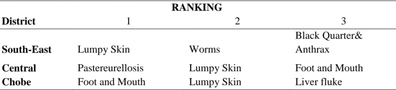
Table 4 Cattle diseases ... 32
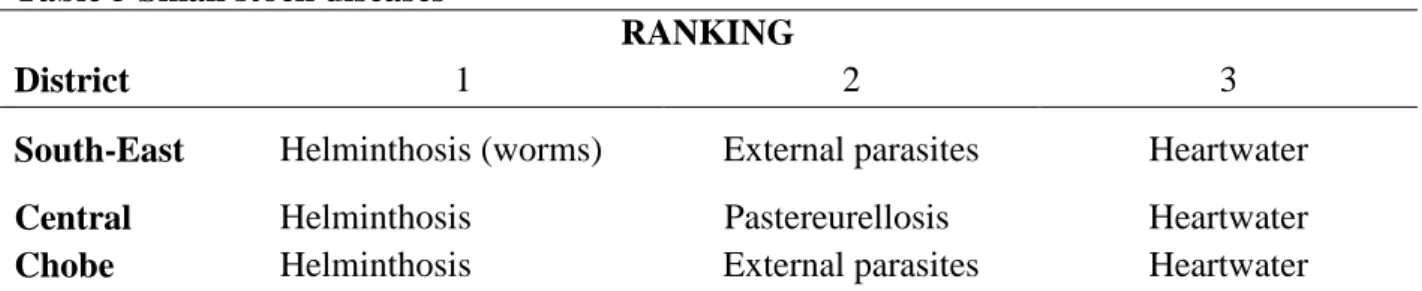
Table 5 Small stock diseases ... 33
Table 6 Estimation of livestock production functions ... 34
1. Introduction
1.1 Livestock situation in Botswana
Most of Botswana’s population live in rural areas where they are largely dependent on agriculture as a source of food, employment and income (Panin, 2000). Livestock production is dominant in Botswana’s agricultural sector, especially rural areas. Small stock such as goats and sheep are also important because they provide an alternative opportunity to augment the incomes of smallholder farmers in the country (Panin, 2000).
In 1966 when Botswana gained independence, the cattle population was about 1.3 million (Government of Botswana, 1991). The cattle population was estimated to be 2.2 million in 2012 for both traditional and commercial sectors (Statistics Botswana, 2012). In the same year, the agricultural sector contributed about 2.7 % to gross domestic product (Statistics Botswana, 2013b). The sector also employs about 26 % of the total formal sector employment (World Bank, http://data.worldbank.org/indicator/SL.AGR.EMPL.ZS?locations=BW, 2016).
The government of Botswana has developed, revived and implemented policies that aimed to boost livestock including small stock productivity and efficiency as well as to increase employment creation (Scoones et al., 2010). Some of these polices include: tribal grazing land policy of 1975, national policy on agricultural development of 1991, artificial insemination and bull subsidy scheme, small stock development programme of 1998, services to livestock owners in communal areas of 1980, livestock water development programme and livestock management and infrastructure development of 2009.
The establishment of infrastructure such as the Botswana Meat Commission (BMC) in 1966 as a slaughtering and marketing channel for all of Botswana’s beef exports favored the cattle industry (Nkombeledzi & Aikaeli 2013). Cattle now have market value unlike in the past when it was used for social or cultural purposes. They are able to sell their cattle in exchange for money. Botswana also had a country specific quota under the beef and veal protocol contained in the Cotonou Agreement that expired in 2007. This quota allowed the country to export specified quantities of boneless meat (fresh and frozen) to the European Union (EU) at reduced import duties. The country has been able to remarkably export these products because
2
it has comparative advantage in beef production due to the availability of rangelands (Seleka, 2005).
Botswana’s livestock sector is comprised of the traditional and commercial production systems. These systems are differentiated by the type of land tenure, degree of market integration and the level of technology adoption.
Most of the cattle are found in the Central region at an estimated number of 545,785 heads whereas the Western region has the lowest (113,517) population of cattle (Statistics Botswana, 2013). The central region has more cattle because it is sparsely populated hence there is more grazing land in this area. In terms of goats and sheep Gaborone region has the largest populations and the lowest populations are found in the Western region (Statistics Botswana, 2013).
Botswana’s livestock sector has economic potential if there are advancements in production technologies. It is capable of increasing the supply of beef to meet both the domestic and international market demands. It can also contribute to the socio-economic goals of the country by increasing employment especially amongst the youth and women, bring new livelihood opportunities, improve food security and diversify the economy away from minerals.
1.2 Research problem
Botswana is a semi-arid country that is hot and dry for most of the year. According to Batisani (2011) mild droughts are the most prevalent in Botswana followed by moderate ones while the frequency of severe and very severe droughts is low. Batisani (2011) further asserts that most parts of the country are vulnerable to hydrological droughts. Thus knowing this information is vital because it helps in identifying areas at risk of water deficit, the likely impacts of such deficit and hence the likely mitigation measures.
Notwithstanding this, livestock production is restrained by recurring droughts and lack of surface water. For instance after severe droughts in the 1980s, the government has continuously introduced various drought-relief programs, such as grants for small stock and other livestock (Simelton et al., 2011).
Rainfall in Botswana is erratic, unpredictable and varies according to the different regions. The poor rains tend to affect drinking water and the availability of grazing land for livestock. The semi-arid condition also makes productivity of the natural resource base very dynamic with the provision of ecosystem goods and services largely determined by the extreme environmental conditions that affect water, soil and landscape form (Sallu et al., 2010). Livestock producers in Botswana are susceptible to risk because they rely on rainfall for the survival of animals. Risk in this context is defined as exposure to adverse and extreme weather conditions, uncertainty of livestock input and output prices and animal disease epidemics.
Diseases also pose as a threat to selling beef to EU market because of the increasing international exports standards. Foot and mouth disease in Botswana affects farmers because during the disease outbreak cattle are killed leaving the farmer unemployed and without a source of income. Poor households are highly vulnerable and thus they are more exposed because they have fewer assets that they can use to shield themselves from shocks. The lack of ownership of resources by livestock farmers also means that they cannot get financing; they need resources to act as security when applying for credit from financial institutions. Lack of access to credit hinders them from acquiring inputs needed to run the farm efficiently. It is important to know how households respond to shocks to understand what households do when they encounter such situations.
The remoteness of farms from major cities and towns also makes it difficult for farmers to have access to markets and supplies. Households are also at times affected by shocks such as livestock diseases, floods, and drought that destroy the assets they own hence affecting them socially and economically.
A larger proportion of the rural household’s wealth is in cattle which provide benefits such as employment, food, and income. Hence livestock plays a crucial role in the lives of rural and urban populations of Botswana. Livestock among smallholder farmers are used as a buffer against risk during times of shocks. Understanding the nature and effects of production risk among smallholder farmers and how to cope is important to improving livestock farming and rural livelihoods.
4
In order to determine and identify relevant improvements and intervention measures to address policy priorities, it is necessary to include risk to determine technical efficiency in order to understand how farmers are affected. It is important for policy makers to know how livestock producers respond to risk in order for them to be able to come up with different diversification strategies for dealing with risk, to help farmers manage risk better by reducing and mitigating risk and lessoning the impact of the shocks. This will help to come up with cost effective strategies that can easily be implemented by farmers.
Building on previous studies (Bahta & Malope (2014), Nkombeledzi & Aikaeli (2013), Motsatsi (2015), Temoso et al., (2016), Bahta et al.,(2015)) that measure technical efficiency of livestock farmers in Botswana, this thesis seeks to address an area that has not been critically examined, which is the production risk associated with input use in the context of efficiency. The study seeks to investigate technical efficiency of livestock farmers using stochastic frontier with production risk to indicate the effects of the input use on the output variance of livestock producers in Botswana. In this context, the study seeks to address the following the questions;
What shocks affect Botswana livestock producers’ and how do they cope with these shocks?
What animal diseases affect livestock producers?
What factors are important in explaining production risk and technical inefficiency?
1.3 Objectives of the study
The purpose of this research is to:
To identify the types of shocks and coping strategies that livestock producers are exposed to
To develop and estimate a stochastic frontier production function in a risky environment
Identify factors that influence technical inefficiency of livestock farmers
To capture the risk faced by cattle farmers in Botswana, both subjective and objective measures will be used. The subjective measures include weather or climatic variables such as rainfall, flooding and extreme temperatures. These environmental factors are able to affect beef output. The type of inputs in relation to the way they affect variability (risk) is important
for input allocation. Therefore it is important to consider variability when making production decisions as it has the ability to influence output levels. Socio-economic characteristics also have the ability to enhance production. In order to account for all these factors, the study employs a stochastic frontier model that incorporates flexible risk component.
1.4 Organization of the study
The study is organized into six chapters. Following introduction on chapter one, chapter two discusses literature review regarding risks faced by farmers in agriculture and concepts related to agricultural risk but also various types and approaches of efficiencies are discussed. The chapter also looks at past studies that have applied technical efficiency. Chapter three looks at the methodology that is applied in the study as well as the empirical model specification and the description of the variables. The Just-Pope production function framework along with other extensions from the literature and their implementation on the stochastic frontier approach are discussed. The next chapter discusses the study area and summary statistics of the socioeconomic characteristics the description of the variables. Chapter five discusses the shocks and coping strategies of farmers including animal diseases that affect cattle and small stock. Econometric results on the determinants of production risk and technical efficiency are also discussed. Finally, chapter six presents the conclusion of the study.
6
2. Literature review
This literature review discusses risks faced by farmers in agriculture and concepts related to agricultural risk. Then it defines the various types of efficiencies and examines the different approaches available for the estimation of production frontier and computation of relative efficiency scores. Finally, it looks at past a study that applies technical efficiency and those simultaneously dealing with production risk and stochastic production frontier. The review of the empirical studies will be limited to Southern Africa and Botswana and some studies focusing on the stochastic production frontier
2.1 Risk in Agriculture
Agricultural production is stochastic and this poses as a major source of risk. Agriculture is often characterized by high variability of production outcomes. Variability in yields is not only explained by factors outside the control of the farmer such as input and output prices but also by controllable factors such as varying levels of inputs (Fufa & Hassan, 2003). Most sources of agricultural risks affecting farmers in both developed and developing countries do not differ as they basically stem from weather, market, and institutional and political-related risks and these are not exclusive to any particular country (Cervantes-Godoy et al., 2013).
Risk can be defined as a situation whereby agricultural producers cannot predict with certainty the amount of output their production process will yield, due to external factors such as weather, pests, and diseases (World Bank, 2005). The decisions they make regarding their farming operations cannot be predicted with accuracy. Risk can also be defined as imperfect knowledge where the probabilities of the possible outcome are known (Hardaker et al., 2004). The impact of natural hazards such as weather variability, climate extremes, and geophysical events on economic well-being and human sufferings has increased alarmingly (Linnerooth-Bayer et al., 2011).
To understand farmer’s risk behavior, it is important to know their attitudes and perception to risk. Farmer’s risks attitude is a unique reflection of their personality usually influenced by socio-economic factors and life experiences and risk attitude influences how the farmer manages his business (Bard & Barry, 2000). Attitude towards risk deals with the farmer’s
interpretation of content of the risk and how much the farmer dislikes the risk (Pennings et al., 2002). Risk attitude can be classified as risk-averse (that is, those farmers who try to avoid taking risk); risk-loving farmers (that is, those who are open to taking risky business) and lastly risk-neutral(that is, those who are neither risk-averse nor risk-loving) (Kahan, 2008).
The complexity of rural life cannot be properly understood through a single theoretical perspective as perception varies with the socioeconomic, cultural, gender, environmental and historical context (Legesse, 2005). Risk perceptions reflect the consumers’ interpretation of the chance to be exposed to the content of the risk and may be defined as a consumer’s assessment of the uncertainty of the risk content inherent in a particular situation (Pennings et al., 2002). Knowing farmers attitude and perception on risk is therefore important as it gives a better understanding of their management strategies. If farmers know the types of risks that they are likely to face, then they can come up with effective coping strategies.
Agricultural risk and uncertainty is due to different factors; it can be due to production uncertainty (weather conditions, pests, diseases and technological change), that is, farmers are not able to know for sure the amount and quality of output that will results from a given bundle of inputs (Moschini & Hennessy, 2001). This can lead not only in the uncertainty of production but also in output prices.
Risk can also be attributed to price uncertainty of farm inputs and output if farmers do not have knowledge about these prices especially at the time when they must make decisions regarding the inputs to use and the quantities to produce. Price uncertainty, is all the more relevant because of the inherent volatility of agricultural markets where such volatility may be due to demand fluctuations, which are particularly important when a sizable portion of output is destined for the export market (Moschini & Hennessy, 2001).
Market risks depend on output and input price variability, but can also include other aspects of farmers’ relationships with participant’s food industry (OECD, 2000). Moreover due to market liberalization and globalization, agriculture has become more risky, causing smallholder farmers to become even more vulnerable (Kahan, 2008). Farmers are susceptible to market risk because they do not have control over the prices of the farm products. Despite market risk being exogenous, farmers can influence yield variability and distribution of returns by the choice of inputs in each enterprise (Fufa &Hassan, 2003). Farm product prices
8
are influenced by cost of production, supply of a product and demand for the product (Kahan, 2008).
Furthermore, livestock diseases are also associated with agricultural risk. Risks of highly contagious diseases are invariably associated with high economic damage, particularly in exporting countries, due to the disruptions these may cause to trade (OECD, 2011).
Lastly, farmers are also exposed to institutional risks such as political risk; loss of key personnel due to death or illness poses farmers to risks that cause disruption to production (World Bank, 2005). Risk and uncertainty do not only affect production output they also influence producers’ behavior regarding the use of inputs. People are both a source of business risk and an important part of the strategy for dealing with risk (Dorfman & Cather, 2013). It is therefore important to identify main sources of risk and come up with risk management strategies to sustain the livelihoods of smallholder farmers.
Risk management strategies adopted by farmers exhibit their perceptions of risk (Beal, 1996) Risk management is a way in which we take care of risk in decision making (Kostov & Lingard, 2003). Farm households adopt diverse strategies such as risk-reducing and loss management strategies to manage risk affecting their income and consumption. These strategies depend on the characteristics of the risk they face, their attitude towards risk and the risk management strategies and tools available (OECD, 2009). Risk-reducing refers to strategies that are designed to smooth income by reducing the ex-ante possibility of a loss and loss management strategies refers to strategies that are designed to mitigate the ex-post consequences of a loss by smoothing consumption in the event of an income shock (Valdivia et al., 1996).
Risk management can be distinguished between informal and formal mechanisms and also between ex-ante and ex-post strategies (World Bank, 2005). Informal strategies are identified as arrangements that involve individuals or households or such groups as communities or villages while formal arrangements are market-based activities and publicly provided mechanisms (World Bank, 2005). The ex-ante or ex-post classification focuses on the point at which the reaction to risk takes place: ex ante responses take place before the potential harming event whereas ex post responses take place after the event. Ex-ante reactions can be further divided into on-farm strategies and risk-sharing strategies (Anderson, 2001). A risk
management system is composed of many different sources of risk that affect farming, different risk management strategies and tools used and available to farmers, and all government actions that affect risk in farming ( OECD, 2009). Table 2.1 shows risk management mechanisms with which farmers can adopt to manage agricultural risk that affects them. Successful adaptations may be viewed as those actions that decrease vulnerability and increase resilience in response to a range of immediate risks (Stringer et al., 2009). The table shows that there are different risk reduction, mitigation and coping strategies adopted by different institutions (farm/household, market, community and government).
Table 1 Risk management mechanisms
Farm/Household Market Community/Informal Government
Risk Reduction
Avoiding risk
Income diversification Low risk
Low return cropping patterns
Production techniques
Training on risk management
New technology
Crop sharing Macroeconomic policy Disaster prevention, prevention of animal diseases Weather data systems Agricultural research Risk mitigation Diversification of production
Saving in the form of liquid assets and buffer stocks
Crop diversification Plot diversification Borrowing from neighbors/family
Intra community charity
Futures and options Insurance Vertical Integration Product/marketing, Contracts Spread sales Diversified financial investment Off-farm work Common property resource management Social reciprocity Informal risk pooling Rotating savings/credit
Tax system income smoothing
Counter-cyclical programs
Border and other measures in case of contagious disease outbreak
Risk coping Sale of assets Reallocation of labor Reduce consumption Borrowing from relatives Migration Selling financial assets Saving/borrowing from banks Off-farm income Sale of assets
Transfers from mutual support networks
Disaster relief Social assistance Other agricultural support programs
Source: Adopted from OECD (2009) 2.2 Measures of technical efficiency
Farrell (1957) defines efficiency the success of a firm in producing as large as possible an output from a given set of inputs. A firm is said to be efficient if it produces along the frontier as shown in Appendix 1. A production frontier refers to the maximum output attainable by a given technology and an input bundle (Bera & Sharma, 1999). It reflects the current state of technology in the industry; firms operate on their frontier if they are technically efficient or
10
beneath the frontier if they are not technically efficient (Coelli et al., 2005). Any firm located on the frontier would have an efficiency score of one while any firm not located on the frontier will be characterized by an efficiency score below one. These efficiency scores could be measured in percentages.
There are different approaches in the literature that have been used to estimate efficiency frontiers. Farrell (1957) identifies two types of these production efficiencies as: i) technical efficiency which refers to the ability to minimize input use in the production of a given output vector or the ability to obtain maximum output from a given input vector (Kumbhakar & Lovell, 2003) and ii) allocative efficiency which is the ability of a firm to choose an optimal set of inputs. On the other hand, a farm is said to be technically inefficient when it is not able to produce maximum output from a given set of inputs and allocative inefficiency when the marginal revenue of an input is not equal to the marginal cost of that input (Schmidt, 1979). Firms need to choose technology that can produce at minimum costs in order to eliminate technical inefficiency and then adjust the mix of factor inputs to suit the prevailing market prices in order to eliminate allocative inefficiency (Anandalingam & Kulatilaka, 1987).
Technical efficiency, its measurement, and the factors determining it are of crucial importance in production theory (Garcia Del Hoyo et al., 2004). The measure of technical efficiency of a farm indicates that if any farm is successful in converting all the physical inputs into output and the efficiency of converting is equal to the hypothetical frontier production function, then it is said to be an efficient farm and if any farm falls short of this requirement then the farm is termed as technically inefficient farm (Reddy et al., 2008).
There are two main frontier approaches that measures efficiency: the parametric and the non-parametric. The distinction between these methods is mainly in the assumptions placed on the data in terms of (i) the functional form of the best-practice frontier, (ii) whether or not account is taken of random errors and (iii) if there is a random error , the probability distribution assumed for the used to disentangle the inefficiencies from the random error (Berger & Humphrey, 1997). The most commonly used approaches are the parametric stochastic frontier analysis (SFA) and the non-parametric mathematical programming approach, commonly known as data envelope analysis (DEA).
The advantage of the parametric approach is that it handles stochastic noise and allows statistical tests of hypothesis concerning the production structure and the degree of inefficiency (Sharma et al., 1999) whereas the advantage of the non-parametric form is that it does not require specification of a particular functional form of technology and distributional assumptions of the inefficiency term (Ajibefun, 2008). The weaknesses of the parametric approach are that functional form must be specified and assumptions on the distributional inefficiencies must be made. Furthermore, impossibility to estimate parameters and test hypothesis concerning the model is the weakness of the non-parametric form.
The stochastic frontier production function as proposed by Aigner et al., (1977) is characterized by an error term which has two components, a non-positive error term to account for technical inefficiency and a symmetric error term to account for other random effects. The non-positive error term indicates that each firm’s output must lie on or below its frontier and that any such deviation is a result of factors under the firm’s control such as technical and economic efficiency, the will and effort of the producer and his/her employees (Aigner et al., 1977) . However the frontier is stochastic, that is, it can vary randomly as a result of favorable and unfavorable external events such as climate, topography etc. (Aigner et al., 1977). The stochastic frontier models are more realistic than the deterministic frontiers because the former can separate the pure noise component from the technical inefficiency effects whereas in the latter all deviations in output are regarded as technical inefficiency effects although the deviations in output might be contributed by random errors. The estimation of technical efficiency using the conventional stochastic model proposed by Aigner et al., (1977) fail to adequately address an important aspect of production, which is production risk. This can result in biased estimates of technical efficiency.
DEA is a linear programming technique where the set of best-practice or frontier observations are those for which no other decision making unit or linear combination of units has as much or more of every output (given inputs) or as little or less of every input given outputs (Berger & Humphrey , 1997).
An important characteristic of production risk is that input levels influence the level of output risk, that is, some inputs increase while others reduce the level of output risk (Tveterås, 1999). Production risk has a tremendous impact on agriculture in general and the production patterns and supply behavior of small-scale farmers.
12
2.3 Review of empirical applications of the stochastic frontier analysis 2.3.1 Existing empirical studies on technical efficiency in Southern Africa
Mochebelele et al., (2000) conducted a study on migrant labor and farm technical efficiency in Lesotho. The study employs stochastic frontier analysis to assess the technical inefficiency of farms that send migrants and those that do not. The study uses survey data conducted in 1995 in four districts of Lesotho; 152 farms that sent migrant labor and 148 farms that were not supplying migrant labor. The objective of the study is to assess the impact of circular migration on Lesotho’s agricultural sector. The results show that the average technical inefficiency was found to be 0.24. They also show that farm size and gender of household does not affect technical inefficiency and that remittances facilitate and current agricultural production rather substitute for it.
Speelman et al., (2008) conducted a study to analyze the efficiency with which water is used in small scale irrigation schemes in South Africa. The study uses data envelope analysis (DEA) to estimate farm level technical efficiency measures and sub vector efficiencies for water use. The results obtained show technical efficiency of 49 %.
Chirwa (2007) uses stochastic production function to estimate technical efficiency among smallholder maize farmers in Malawi. The study uses data that was collected on 156 households. The data included plot level output of maize and other crops produced, inputs used on production process (land, capital, labor, fertilizer), socioeconomic and plot specific characteristics. The objectives of the study are to estimate the mean and plot-specific technical efficiency levels, examine the impact of technology adoption and to determine to the role of efficiency drivers among smallholder farms producing maize. The results showed average technical efficiency score to be 46.23 %. It also shows that inefficiency declines on plot planted with hybrid seeds and for farmers who belong to households with membership in a farmers’ association.
Simwaka et al., (2013) analyses factors affecting technical efficiency of smallholder farmers in Malawi comparing time varying and time-invariant inefficiency models. The objective of the study is to estimate technical efficiency and identify factors that explain differentials in
technical efficiency of households affected and not affected by HIV/AIDS. The study applies stochastic production frontier for panel data which was collected on 11,280 households in 2004/5 and 2006/6. The results showed 73 % technical efficiency for non-affected households for time varying and 78 % for time invariant models. For affected households, 69 % for time varying and 71 % for time invariant inefficiency models. Furthermore, the results show that male headed households are more efficient compared to female households. Also, households with morbidity are more technically efficient than households with mortality.
2.3.2 Studies from Botswana on technical efficiency
Bahta & Malope (2014) used stochastic production frontier to investigate the determinants of profitability, efficiency drivers and profit efficiency of beef farmers in Botswana. The study sought to measure competitiveness of beef producers using profitability as a yardstick. The study uses cross sectional farm level data of a study which was carried out in three districts (South East, Chobe and Central) of Botswana. The overall technical inefficiency has been found to be 74 % whereas the mean profit efficiency level was 58 %. Efficiency drivers have been identified as education of household, distance to commonly used markets, information access, herd size and access to income from crop production.
Nkombeledzi & Aikaeli (2013) conducted a study on technical efficiency of the Botswana Meat Commission (BMC). Their objective is to examine the performance of the BMC, ascertain efficiency status and to underlines the causes of inefficiency in the Botswana beef sector. The study applies transcendental logarithmic stochastic production frontier to estimate the efficiency status of the BMC. Secondary data for a period 1979-2009 was used. The inefficiency was found to be 22 % which is argued to be driven by material constraints and insufficient penetration into the global markets.
Bahta et al.,(2015) investigate factors influencing efficiency in beef production in Botswana by applying a stochastic Metafrontier-Tobit method. The objective of the study is to investigate determinants of technical efficiency in different beef cattle production farm types in Botswana. The study uses farm level cross sectional data where farmers are grouped three different farm types to be able be account for technology gaps across them. The average technical efficiency was found to be 0.496.
14
Motsatsi (2015) conducted a study on technical efficiency and evidence of economies of scope in Botswana agriculture. The objective of the study was to estimate district and commercial sector technical efficiency to obtain measures of evidence of economies of scope. The study uses the multiple-output multi-input stochastic input distance function approach to analyze data from 1979 to 1996. The results show that the mean technical efficiency is 0, 88. The study also found there are significance economies of scope between the production of cattle and goat/sheep and cattle and crops.
Bahta & Hikuepi (2015) conducted a study to measure technical efficiency and technological gaps of beef farmers in Botswana using the meta-frontier approach. The study shows that average technical efficiency is 0.496. The estimates also show that there are significant differences in production technologiesin the three investigated district.
Temoso et al., (2016) used panel data to assess technical efficiency and technological gabs across 26 agricultural districts in Botswana over a period of nine years. The average technical efficiency ranges between 0.79 in Southern region and 0.40 in Maun region.
2.3.3 Studies on production risk and technical efficiency
Kumbhakar (1993) applied the flexible risk model to measure production risk and technical efficiency using panel data among farmers in Sweden. His results show that marginal risks are positive for concentrate fodder, labor and capital and negative for material, grass fodder and pasture land. With regards to technical efficiency they found the farms to have high relative efficiencies.
Moreover Kumbhakar (2002) applied the flexible risk model to measure production risk, technical efficiency and risk preferences using cross section data to Norwegian salmon farmers. The results they obtained show that all farmers are risk averse, production risk is found to be increasing feed and decreasing with labor and capital. Technical inefficiency is found to be negatively related labor and capital and positively related to feed. The average technical inefficiency score is found to be 7.9 %.
A study by Villano & Fleming (2006) also uses stochastic frontier production function with a heteroskedastic error structure to analyze the inefficiency of rain-fed lowland rice in the
Philippines. The study uses an eight year-old data panel from 46 rain-fed rice farmers. Their results found technical efficiency to be 79 %. The results further show that there is high degree of variability in technical efficiency estimates due to the instability of the farming conditions. The inputs that increase risks have been found to be area planted to rice, labor and the amount of fertilizers whereas herbicide was found to be a risk reducing input. The study also reveals that education and age enhance technical efficiency.
In the work done by Jaenicke et al., (2003), they investigate the effect of production risk and inefficiency using stochastic frontier production function to compare to different cultivation systems for cotton. Their results show that when the stochastic frontier model is compared to the typical Just-Pope model, it reorders the relative riskiness of cover crop regimes associated with the cotton system.
Bokusheva & Hockmann (2006) evaluate the efficiency of Russian farmers by investigating production risk and technical inefficiency using panel data. Their study results show that technical inefficiencies enhance variability of agricultural production in Russia and that production risk contributes to the volatility of agricultural production. Likewise Battese et al., (1997) apply stochastic production function for cross sectional data within the framework of a flexible risk model. They apply this model to peasant farmers in Ethiopia. Their result shows that equipment, cattle and land have a positive marginal risk that is they have an increasing effect on the variance of the value of output.
In addition Ogundari & Akinbogun (2010) study 64 randomly selected fish farms in Nigeria to investigate technical efficiency and production risk using the stochastic frontier model with flexible risk properties. Their results show that labor, fertilizer and feed influence fish output. Their study found that fertilizer and feed to be risk-increasing inputs whereas labor is a risk reducing input. They also found that labor, farming experience, education and access to markets significantly decreases technical inefficiency.
Mochebelele et al., (2000) showed that farm size and gender do not affect technical inefficiency. Technical efficiency declines for household who are members of farmer’s associations. Drivers of technical efficiencies are education of household, distance to the nearest market, information access, herd size, access to income from crop production. Other inputs that increase risks are identified as area of crop planted, labor, fertilizers and feed.
16
The empirical reviews above, determined technical efficiency in agricultural production. The studies showed that there are different factors that influence technical efficiency such as membership to a farmers’ association and male headed households are more efficient that female headed households. Some studies also show that education of household, distance to commonly used markets, information access, herd size and access to income and insufficient access to global markets are the main drivers of efficiency. This study will contribute towards literature by analyzing production risk and technical efficiency amongst smallholder livestock farmers in Botswana.
3. Methodology
This chapter develops the Just-Pope production function and other extensions that are used in the study. It also discusses empirical model application and specification as well as explanation of variables that associated with input, risk and technical efficiency.
3.1 Just-Pope production function 3.1.1 Model specification
At the outset, this study employs the stochastic frontier framework on production risk as suggested by Just & Pope (1978,1979) and the extension thereof that incorporates producers attitudes towards risk by Kumbhakar (2002). Traditional stochastic production functions state that, if any input has a positive effect on output then a positive effect on variance is also imposed (Just & Pope, 1979). The underlying concept regarding this approach is that production function can be related to the output level and the output variability thus allowing for the estimation of the impacts of an input variable, expected output and variance (Cabas et al., 2009). Nonetheless, the effects of input on output should not be tied to the effects of input on variability of output a priori (Fufa & Hassan, 2003). A production function therefore has to specify the effects of input on the mean of output and also specify the effects of input on the variance of output (Just & Pope, 1979). The production function proposed by Just & Pope is generally presented as:
) ( , ) , ( f x h x Y , E()0,V()1 (1)
Where Y is the output level, f(x, α) are the effects of the inputs on the mean output (deterministic component), h(x, Φ) is the variance of output (risk component of output), x represents vector of inputs which have an influence on both the mean output and risk, α and Φ are parameters and ε is the random error term. This is because E(y) f(x) and V(y)h(x).
3.2. Stochastic frontier analysis 3.2.1 Model presentation
18
In order to estimate the stochastic production frontier, the approach proposed by Kumbhakar (2002, p17) could be applied to the study of beef smallholders in Botswana. He specified the following production frontier model:
Y= + g ( , θ) v - (2)
where f(x,) is the mean output, is the inefficiency function for explaining the effects of inputs and socio-economic variables on technical inefficiency, g(x, θ) is the production risk function, µ, θ and α are parameters, vi is the random disturbances terms that follow a normal distribution and they are assumed to be independently and identically distributed with zero mean and variance . The inefficiency term ui is a non-negative variable associated with farm-specific technical inefficiencies. It is assumed to follow a truncated-normal distribution with mean u and variance . The economic relationship for this error term specification indicates that the system of production is subject to a non-positive component, which makes the production to lies on or below the frontier ( Battese & Coelli, 1992).
From equation (2) the mean and variance of the output for the ith farmer, given the values of the inputs and technical inefficiency effectsare:
+ (3)
(4)
The marginal production risk with respect to the j-th explanatory variable is defined to be the partial derivative of the variance of production with respect to xj. The marginal production risk can either be negative or positive depending on the sign of the associated parameter θ. That is, x u x y Var ( | , ) > 0 or < 0 (5)
(6) Where indicates that the producer is technically efficient.
Technical inefficiency (TI) is represented as:
(7)
Thus, technical efficiency becomes;
TE = 1-TI (8)
Technical efficiency of the i-th farmer is not only a function of its technical inefficiency effects, but also of the values of the explanatory variables and the parameters of the production frontier including the risk parameters.
3.3 Empirical model specification
Implementation and preliminary estimation of the conceptual model presented in the previous section did not lead to meaningful and interpretable estimates of the parameters defining the stochastic frontier production function defined by expression (2)1. Given this state of affairs, an alternative stochastic production model to analyze beef smallholders in Botswana has been implemented empirically and estimated using a maximum likelihood (ML) estimation approach. This alternative approach which is based on the stochastic production frontier specification developed by Wang (2002), Chang and Wen (2011) and Kumbhakar et al., (2015) is developed and explained in this section.
1 The preliminary estimation of the model represented by an empirical version of expression (2) using
tractable and simple functional forms for the various terms f(x,), g(x, θ) and q(x, α) based on ML and iterative nonlinear least squares methods result in estimated parameters with unexpected signs and wrong magnitudes, which, for this reason were not prone to any economic interpretation. In addition, it also occurred that we have been confronted with non-convergence estimation problems using the TSP and STATA econometric softwares.
20
There are various functional forms that can be used to estimate stochastic frontier models. This study uses Cobb-Douglas production function because it is easy to use even though it imposes restrictions on the production elasticities of inputs to be constant and the elasticity of substitution among inputs to be equal to one. In this study, the Cobb-Douglas production is used as follows:
(9)
where ln is the natural logarithm, ’s are parameters to be estimated2; x are factors of i production which include livestock herd, other capital and variable inputs; Y is beef output i calculated in beef equivalents, vi is the random disturbance term with zero mean and a variance , and ui is the non-negative inefficiency term. Concerning on how beef output was computed, full explanations are provided in Table 2. In the same vein, the definitions and data used for the three input variables are also presented in the same table.
In the above production function as just indicated, the determinants of the inefficiency term and of the risk factors facing beef smallholders in Botswana are not going to be modeled using the Kumbhakar-adjusted, Just and Pope production function approach, but are rather captured by using an alternative stochastic production frontier specification developed by Wang (2002), Chang and Wen (2011) and Kumbhakar et al., (2015). In this latter stochastic frontier model specification, the inefficiency term ui is assumed to follow a left-truncated normal distribution with a constant variance and an expected mean which varies according to the following expression:
(10)
0 and i are parameters to be estimated, Z are explanatory variables describing the technicali inefficiency. These include livestock herd, gender, age, years of education, rainfall, temperature, districts, sick animal, off farm income and household size.
2 The’s parameters are also representing the elasticities of output with respect to each input. The sum of
the’s also provides an estimate of the returns to scale of the underlying Cobb-Douglas production
The second additional component introduced in expression (9) concerns the way risk variables are influencing the production decisions of beef smallholders in Botswana. As we decided not to rely on the Just-Pope production function framework, a possible channel to make the risk variables incorporated into the stochastic production frontier model represented by expression (9) is to assume that the variance ( ) of the random error term vi is a function of risk variables such as climatic variables (i.e. rainfall and temperature) and proxies for sick animals. In so doing and to preserve the positive nature of the variance ( ), an exponential functional form is adopted to specify this risk function. In so doing, the random term vi becomes heteroscedastic and is also assumed to follow a normal distribution with a zero mean.
To recapitulate, the empirical stochastic production frontier model that is finally adopted is represented by the following expressions:
(11a)
(11b)
(11c)
(11d)
(11e)
Where N() and N+() represent the normal and left-truncated normal distributions, respectively; EXP designates the exponential function; 0 and k are parameters of the risk function to be estimated; Zv,k are risk variables that are a subset of the Zi variables determining the mean inefficiency term ( ). As pointed out earlier, these risk variables are rainfall, temperature and proxies for animal diseases; the other terms appearing in expressions (11a) to (11e) have been previously defined.
To estimate the above stochastic production frontier model is undertaken using a maximum likelihood estimation approach. The associated Log-Likelihood function combines a mixture of normal distributions defining the inefficiency term (with a varying mean inefficiency) and
22
the heteroscedastic residual term. The expression defining this Log-likelihood function is quite complex and can be found in Kumbhakar et al., (2015, Chapter 3). The ML procedure to estimate the Log-likelihood function is undertaken with the menu-driven program on stochastic frontier production functions found in the STATA software (STATA, 2017).
Once the above stochastic production frontier model has been estimated, the technical efficiency score for each beef producer is calculated as follows: (Chang and Wen, 2011, Kumbhakar et al., 2015)
(12)
Where the E{}is the expectation operator and are estimated residuals obtained through the following expression:
(13)
The risk term of each beef producer is the predicted value of the exponential function represented by expression (11e). It is also possible to estimate the marginal effect of each exogenous factor on mean production efficiency using the procedure suggested by Wang (2002) and Kumbhakar et al., (2015).
Table 2 Explanation of Variables
Variable Description
Output Beef output calculated in beef equivalents. Due to measurement difficulties, this study follows the revenue approach recently applied in the literature (Abdulai & Tietje (2007), Gaspar et al., (2009), Hadley (2006)) and defines output as follows
t yp Q R r j i
) (Where Qi( j) is the annual value of beef cattle output of the ith farm in the jth production system (measured in Botswana Pula; r denotes any of the three forms of cattle output, i.e., current stock, sales or uses for other purposes in the past twelve months period; y is the number of beef equivalents’ p is the current price of existing stock or average price for cattle sold/used during the past twelve months; and t is the average maturity period for the beef cattle on Botswana, which is assumed to be four years based on the export consultation.
Livestock herd Following (Hayami & Ruttan, 1970; O’Donnell, Rao, & Battese, 2008; Otieno, Hubbard, & Ruto, 2012) Beef cattle equivalents were computed by multiplying the number of cattle of various types by conversion factors. Following insights from discussions with BMC (Botswana Meat Commission), the conversion factors were calculated as the ratio of average slaughter weight of different cattle types to the average slaughter weight of a mature beef bull. The average slaughter weight of mature bull, considered to be suitable for beef in Botswana, is between 452-500kg. per BMC, the average slaughter weights for castrated adult males (oxen>3 years), Immature males (< 3 years), Cows (calved at least once), Heifers (female ≥1year, have not calved), Male calves (between 8 weeks&<1year), Female calves (between 8 weeks&<1year), Pre-weaning males (<8 weeks), Pre-weaning females (<8 weeks) are 400kg, 350kg, 390kg,300kg,250kg, 220kg,95kg and 95 kg, respectively. The calculated average slaughter conversion factors were then: 1.0, 0.86, 0.76, 0.84, 0.65, 0.48, 0.54,0.21 and 0.21, for Bulls, castrated adult males, Immature males, Cows, heifers, Male calves, Female calves, Pre-weaning males, and Pre-weaning females, respectively)
Other variable inputs Capital equipment Age of household head Years of education Gender
Rainfall Temperature Off farm income Sick animal Household size Regional effects
is total costs in Pula and it captures total feed cost, total wage, total veterinary cost this are equipment related cost in Pula
measured in years
is measured per the level of education
is a dummy where 1= male farmer and 0 = female farmer average rainfall in millimetres
maximum temperature in degrees Celsius income earned from non-farm activities
is a dummy for animal disease where 1=sick animal is number of family members
for investigating regional effects on efficiency, district fixed effect (that is, South East, Central and Chobe) is introduced with Chobe as the reference group
24
4. Data
This chapter is divided into two sections 4.1 and 4.2 with the former discussing the study area and the latter discusses the summary statistics for the socio-economic characteristics.
4.1 Data sample and study area
This study uses farm level cross-sectional data of 540 randomly selected livestock farmers from a survey which was conducted in 2012. This is survey data for a project “The Smallholder Livestock Competitiveness Project” funded by the Australian Centre for International Agricultural Research (ACIAR) and implemented by the International Livestock Research Institute (ILRI) in partnership with the Botswana Ministry of Agriculture’s Department of Agricultural Research.
The study also uses rainfall and temperature data sourced from the Department of Meteorological Services. There are seven rainfall stations and eleven temperature stations in the study area. Distance between all weather stations and villages in the study area were calculated, then each household was assigned to the closest weather station.
The study was conducted in Central, South East and Chobe districts of Botswana (see Figure 1). The Central district is the largest administrative district in terms of the population and area. It has a total of 17 211 cattle holdings, 18 419 goat holdings and 4567 sheep holdings (Statistics Botswana, 2013a). The study specifically covers the villages of Serowe, Letlhakane, Selebi-Phikwe and Nata, which fall under the Tutume agricultural region. Serowe has 2179 cattle, 2052 goat and 392 sheep (Statistics Botswana, 2013a). On the other hand, Letlhakane has 1718 cattle, 1747 goats and 484 sheep holdings whereas Selebi Phikwe has 852 cattle, 1014 goats and 372 sheep. The major economic activities in these areas are selling livestock, trading store (shop/vendor), selling traditional beer, ploughing and timber harvesting as well providing transport services. The main sources of income for people living in these areas are sale of livestock, pension, and employment. The most cattle common disease includes anthrax, black leg, botulism, brucellosis, foot and mouth, and lumpy skin.
According to Statistics Botswana (2015) the South-East district has a population of 85,014. This district surrounds Gaborone which is the capital city of Botswana. It has 18,586, 21,582
and 5543 cattle, goat, and sheep holdings respectively (Statistics Botswana, 2015). The Balete/Tlokweng region has 3245 cattle, 3983 goats and 716 sheep holdings and the most common economic activities are selling traditional beer, selling crop produce, trading store, selling livestock and selling veld products. Other activities include transport and ploughing services. Cattle diseases that are common in this area are anthrax, black leg, brucellosis, and botulism. The most common sources of income in the South-East district are pension, remittances, employment, and sale of livestock.
Chobe district is found in the North-Western part of Botswana. It has 243 cattle and 167 goat holdings (Statistics Botswana, 2015). Economic activities in this district include trading store, selling traditional beer, ploughing services, selling livestock including other services such as transport and fishing. Foot and mouth, anthrax, black leg, and brucellosis are the most common cattle diseases found in this district. The Chobe district is well known as a tourism hub as it is endowed with rich flora and fauna. However, the rich wildlife population that include the African buffalo which is a major carrier and transmitter of foot and mouth disease makes this area prone of this disease. Pension, business other than farming, remittances, and employment are the main sources of income for the people living in this area.
26 Figure 1 Map of the study area
Source:Mapitse, 20083
3 The map shows the areas where data was collected being South East, Centra l(Serowe,Selibe Phikwe,
Letlhakane,Nata) and Chobe District. The map also shows the different Foot and Mouth Disease (FMD) control areas. FMD is very prevalent in Botswana hence the country is divided into risk zones where the red zones represent FMD vaccination areas and the green zone are the FMD free areas
4.2 Summary statistics of socioeconomic characteristics
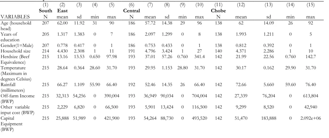
Table 3 shows the socio-economic characteristics of the farmers. Efficiency at the farm level may be influenced by the age of the farmer. In this study, the average age of a farmer is 62 years for South East and Chobe districts whereas for Central it is 57. The results signify that farmers in the study area are mainly elderly and this may affect their overall efficiency. This average age is consistent with other studies on beef cattle farmers in Botswana that show that most of them are elderly. This is because most of the farmers engage actively in farming after retirement. Studies by Mmopelwa & Seleka (2011) and Mahabile (2013) show that average age of cattle farmers in Botswana is over 50 years old.
In relation to education, the average years of schooling of the livestock farmers is 1.211 for Chobe which is the lowest followed by 1.317 for South East and 2.097 for Central. These results show that most of the farmers have lower level of education as they have obtained up few years of education. Education is key in decision making at farm level because it can determine the rate at which the farmer adopts new technology. It also helps farmers to rationalize on inputs which may assist in raising output. In the study by Lockheed et al., (1979) on farmers education and farm efficiency shows that education has a positive effect on technical efficiency.
There are fewer females compared to their male counterparts who are involved in farming in the study area. For Central district 75% of the farmers are males, followed by 78% in South East and 81% in Chobe district. This result is consistent with the study by Otieno et al., (2012) where their study revealed that for the different farm types under study, males were the majority farmers estimated to be 66.4% for nomads, 67.2% for agro-pastoralists and 87.9% for ranchers.
The average household size is four members for all the districts under study. Use of family labor is important for farmers as they are much more hardworking and readily available to assist at the farm (Pollak, 1985).
With regards to livestock herdsize, the South-East district has the lowest average number of herdsize (13.16). On the other hand, the Central district has the highest average herdsize of cattle
28
(37.01). The average livestock herdsize for Chobe district is 21.99. This shows that farmers in the Central District have more livestock compared to the rest of the district in the study area.
The average annual maximum temperatures are 28.64, 29.95 and 30.17 degrees Celsius for South East, Central and Chobe districts, respectively. This shows that on average Chobe district is hotter than the other districts in the study area. With regards to average annual rainfall Chobe district has the highest rainfall of 72.66 millimeters followed by South East district with rainfall amounts of 66.27 millimeters. Lastly, Central district receives average annual rainfall of 52.46 millimeters.
Regarding off farm income, the average for a household in South East is 32,313 4BWP, Central district 36,949 BWP and Chobe district is 27,339 BWP. Total other costs which includes total feed cost, total wage and total veterinary cost is 2,229 BWP, 5,901 BWP and 5,045 BWP Celsius for South East , Central and Chobe districts respectively. On the other hand, average capital equipment for South East is 25,888 BWP, Central district is 54,264 BWP and Chobe district is 51,470 BWP.
4 1 BWP = 0.0826 EUR,
Table 3 Summary statistics of socio-economic characteristics
(1) (2) (3) (4) (5) (6) (7) (8) (9) (10) (11) (12) (13) (14) (15)
South East Central Chobe
VARIABLES N mean sd min max N mean sd min max N mean sd min max
Age (household head) 207 62.00 11.92 31 90 186 57.72 14.38 29 96 138 62 14.09 26 92 Years of education 205 1.317 1.383 0 7 186 2.097 1.299 0 8 138 1.993 1.211 0 5 Gender(1=Male) 207 0.778 0.417 0 1 186 0.753 0.433 0 1 138 0.812 0.392 0 1 Household size 214 4.430 2.308 1 11 191 4.796 3.424 1 27 140 4.371 2.286 1 10 Herdsize (Beef Equivalence) 215 13.16 13.53 0.650 97.98 193 37.01 57.26 0.760 341.4 142 21.99 22.56 0.760 142.7 Temperature (Maximum in degrees Celsius) 215 28.64 0.364 28.60 31.70 193 29.95 1.153 28.80 31.70 142 30.17 0.162 29.90 31.70 Rainfall (millimeters) 215 66.27 1.109 55.90 66.40 192 52.46 14.35 26 66.40 142 72.66 5.660 59.60 76.40 Off-farm Income (BWP) 215 32,313 54,256 0 390,004 193 36,949 90,034 0 704,004 142 27,339 76,204 0 613,804 Other variable input cost (BWP) 215 2,229 6,820 0 66,500 193 5,901 13,424 0 116,500 142 9,299 8,520 0 42,940 Capital Equipment (BWP) 215 25,888 51,989 0 421,900 193 54,264 88,730 0 493,520 142 51,470 183,888 0 2.092e+06
30
5. Results and discussion
The section deals with shocks and coping strategies of beef producers. The chapter also includes animal diseases that affect cattle and small stock. It also discusses econometric results on the determinants of production risk and technical efficiency. This chapter provides answers and assessment on the three objectives assigned to this research.
5.1 Shocks and diseases that affect livestock farmers 5.1.1 Shocks that affects farmers
Farmers5 in the study area were given a list of risky events that affect them at individual level to find out how they perceive risk. They were asked to rank the events in terms of their importance on a scale of 1 to3 with one being the most severe and three being the least severe event that affect them.
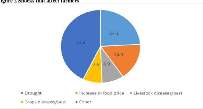
Figure 2 below gives a summary of these shocks for all the districts under study. The most significant shock per the farmers is drought at 42.8%. Due to the semi-arid climatic conditions of Botswana, the country experiences variability in rainfall leading to sporadic drought conditions. Drought in turn impairs rural livelihoods hence most of the households in the study area responded by stating that drought affects their production. The other factors that affect farmers are increase in food prices (16.4%), livestock diseases (8.9%) and crop diseases and/or pest (7.8%). The item “other (24.1%)” is a combination of shocks that affects farmers, it include flooding, pests and/or disease attacks that led to storage losses of crops or fish, theft of livestock, theft of production tools and equipment, theft of cash, destruction of housing, death of adult household member, disablement of adult/child household member, decrease in output prices, increase in input prices, job loss by household member, forced loss of tenancy of land, forced migration of household, communal crisis, fire outbreak and no market for products.
Figure 2 Shocks that affect farmers
5.1.2 Coping strategies
Figure 3 shows the coping strategies that farmers would adopt to avert the consequences of the various shocks that befall them. The highest ranked strategy that farmers would adopt is to work hard (36.5%). This is followed by reducing food consumption (13.3%), selling livestock (12.7%) and others said they will get assistance from government (8.5%).