Who Benefits from More Housing? : A Panel Data Study on the Role of Housing in the Intermunicipal Migration of Different Age Cohorts in Sweden

(1)

© Southern Regional Science Association 2018. ISSN 1553-0892, 0048-749X (online)

www.srsa.org/rrs

The Review of Regional Studies

The Official Journal of the Southern Regional Science Association

Who Benefits from More Housing? A Panel Data Study on the Role

of Housing in the Intermunicipal Migration of Different Age

Cohorts in Sweden*

Peter Karpestam

Department of Urban Studies, Malmö University, Sweden

Abstract: Although Swedish housing standards are high and young adults leave the parental home relatively early,

there are indications that for certain groups housing has, in recent years, become less accessible. We analyse how housing characteristics affect intermunicipal mobility for different age cohorts and estimate a panel data gravity model that models migration as a function of origin and destination characteristics. The results suggest that new construction in the past two decades has negatively affected migration within commuting regions more than migration between commuting regions. For metropolitan areas, there are considerable negative effects on net migration from other commuter regions because new construction has not kept pace with population growth. The effects are stronger for young adults (20-44) compared to older adults (45-74). Further, we find that, while new construction stimulates mobility for all age cohorts, the estimated relationship is weaker for the youngest adults; indicating a need for more variation in new construction to satisfy different needs. Also, we find that the decreased share of rentals since 1992 have negatively affected the short-distance mobility of the youngest adults while the effect is weaker or even positive for the remaining age cohorts.

Keywords: regional migration, housing supply, tenure, age, urbanization, Sweden, gravity model. JEL Codes: R21, R23, R31

1. INTRODUCTION

In recent years, the Swedish public has witnessed an intensified public debate on housing, provoked by low levels of new construction over two full decades. Throughout the country, inflation-adjusted housing prices are historically high, having increased steadily after hitting rock bottom in 1995; and in many places—particularly in central urban locations, in both large and small cities—the wait-times for rental units amounts to several years (The Swedish Union of Tenants, 2014). High housing prices exclude some households from owning, and renting is not always possible; as there are few vacancies and landlords may reject the unemployed, low-income households, or those with a track record of non-payment (Jacobsson, 2012; Swedish National Board for Housing, Building and Planning, 2014,).

Aggregated data suggests that the housing situation has deteriorated more for some groups than for others. For example, in recent years, the percentage of young adults still living in the parental home has increased (Abramsson, Fransson, Borgegard, 2004; Statistics Sweden, 2008; The Swedish Union of Tenants, 2015). Also, while young immigrants and low-income households

*_{The Author would like to acknowledge the Swedish National Board of Housing, Building and Planning for funding major parts}

of this work. Peter Karpestam has a Ph.D. in Economics and is an Assistant Professor in Real Estate Science at Malmö University, Kultur och Samhälle, 205 06 Malmö, Sweden. Corresponding Author: Peter Karpestam. E-mail: peter.karpestam@mau.se

(2)

are overrepresented in rental housing,1 the total housing percentage that are rental units has decreased for two decades due to the tenure conversion of a considerable number of units to co-operative housing2_{and to decreased new construction.}

The question we address in this paper is whether housing market characteristics affect the mobility of different age cohorts differently. Using yearly data at the municipal level between 1993 and 2012, we construct a gravity equation and model intermunicipal migration for different age cohorts as a function of push and pull factors of the origin and destination. We investigate how changes in the size of the existing stock of dwellings (per capita), the level of new construction (per capita), and the tenure distribution (the share of rented dwellings) is related to intermunicipal migration for different age cohorts (20–24, 25–34, 35–44, 45–54, 55–64, and 65–74). We separate between intermunicipal migration within and between commuting areas because previous research suggests that housing considerations are more important for short-distance migration, and that job related reasons and educational purposes are more important for long-distance migration. Even if housing considerations are not the primary catalyst for the majority of long-distance moves, it is relevant to investigate the role of housing in this context because motives for long-distance migration are often labor market oriented and obstacles against labor migration can negatively affect economic growth.

There has been little research on the relationship between housing and internal migration in a Swedish context. While existing studies have often used micro data,3 this paper complements previous research on how housing affects mobility in Sweden by taking a macro perspective. Further, we contribute to the literature by separating between different age groups, because individuals of different ages have varying needs for housing, and because age correlates with the ability to find suitable housing. We know that young adults have relatively low incomes4_{and the}

decreasing share of rentals over the past two decades may affect the mobility of different age cohorts differently, as young people are overrepresented in the rental sector. Furthermore, intermunicipal migration rates are considerably higher for young adults than for other adults. We are unaware of studies that have attempted to analyze whether housing characteristics influence the mobility of different age cohorts differently. Moreover, our paper relates to an important policy issue: whether or not the real estate market is for everyone and whether housing market changes benefit or hurt the mobility of some age cohorts more than others.

The rest of the paper is organized as follows. Section two provides a literature review. Section three describes developments on the Swedish housing market during the past two decades. Section four describes the empirical model and the data, and discusses some important theoretical considerations. Section five presents the empirical results, and section six concludes.

1_{For instance, the share of young adults between 20 and 24 years of age living in rentals was 36 percent in 2014. The average for}

all age cohorts was 26.5 percent, 46.6 and 21 percent with non-Swedish background and Swedish background lived in rentals, respectively. Source: Statistics Sweden, www.scb.se.

2_{This is described in Andersson and Magnusson Turner, 2008.}

3_{For instance, Millard-Ball (2002) used data from nine properties in the inner-city of Stockholm and found that tenure conversions}

led to increased mobility and reduced the number of inner-city rental vacancies. Magnusson Turner (2008) simulates Markov Vacancy Chains in the City of Stockholm. She finds that new vacancies were often claimed by households moving in from other local markets and that vacancy chains generally transfer within the same submarkets. Emmi and Magnusson (1995) evaluate different chain vacancy models using census data for Västerås, Gävle, and Jönköping from 1975, 1980, 1985, 1990.

4_{In 2013, earned per capita incomes for individuals between 20 and 24 amounted to 44 percent of earned per capita incomes for}

(3)

2. LITERATURE REVIEW

At the macro level, researchers have studied the effects of parameters such as housing prices, tenure forms, housing policies, and demographic and economic conditions on regional mobility (Engelhardt, 2003; Smith & Smith, 2007; Cunningham & Engelhardt, 2008; Ferreira, Gyourko, & Tracy, 2010; Caldera Sánchez & Andrews, 2011; Ermisch & Washbrook, 2012; Hilber & Lyytikäinen, 2012). Micro-level studies have often focused on the decision process and how individual characteristics influence people’s housing choices (Dieleman, 2001). For example, several studies have established that residential mobility depends on the current state of the economy (mortgage rates, business-cycle fluctuations, etc.) and on migrant’s characteristics such as educational, social networks, and knowledge about the housing market (Whittington & Peters, 1996; Murphy and Wang, 1998). Further, previous research suggest that the ability to find suitable housing is relatively limited at the beginning and at the end of housing careers (Clark & Dieleman, 1996). There is an extensive amount of literature that has analyzed determinants of internal migration using gravity models, as well as other approaches (Hämäläinen & Bäckerman, 2004, Ashby, 2007; Bloze, 2009, Partridge et al., 2012). Providing a full review is beyond the scope of this paper. Instead, we focus on some key findings regarding the relationship between mobility and housing from studies that have attempted to separate internal migrants by age.

One strand of the literature has focused on how land-use regulations and other housing supply constraints affect the capacity of regions to grow and to attract (labor) migrants (Kim, 2011 provides a literature review). One recurrent finding is that in regions where housing supply constraints are relatively strict, an increase in housing demand results in increased housing prices as opposed to more new construction (Levine, 1999; Glaeser, Gyourko, & Saks, 2005; Saks, 2008). Some studies have related housing supply factors to the labor market. An important finding is that the population (and labor force) is less likely to grow in regions where land-use regulations are relatively strict. Thus, a labor demand increase will not necessarily translate into higher employment because the regional capacity to attract labor migrants is low due to housing supply constraints (Glaeser, Gyourko, & Saks, 2006; Vermeulen & Ommeren, 2009). Similarly, using cross-sectional household data for 25 OECD countries, Caldera Sanchez and Andrews (2011) find that residential mobility is higher in countries with a more responsive housing supply.

Moreover, research has shown that renters are more mobile than are homeowners (Hamnet, 1991; South & Deane, 1993; Rohe & Stewart, 1996; Lundberg & Skedinger, 1999) which is often explained by the low transaction costs of moving for rentals.5 This indicates that the decreased share of rented dwellings may negatively affect mobility. However, in a Swedish context, we do not know whether the turnover rate is relatively high in the rented sector6 because of comparably low moving costs, or because of the overrepresentation of young adults and foreign-born individuals (or both). The Swedish system of rent control is considered strict internationally, which may effectively reduce the turnover rate in the rented sector (Lind, 2003).

However, studies that 1) link housing to mobility and 2) separate between age groups in a gravity model are either rare or non-existent. In a Swedish context, studies that investigate determinants of internal migration have tended to ignore housing (Dahlberg & Holmlund, 1978;

5_{Another possible explanation is that relatively mobile individuals choose to stay in rental housing.}

6_{The turnover rates for all publically owned housing (rentals) was 17 percent in 2013. The turnover rate for cooperatives was about}

9.6 percent the same year. The turnover rate for “småhus” (mainly owned dwellings) was about 2.7 percent. Source: Statistics Sweden (www.scb.se) and the Swedish Association of Public Housing Companies (SABO).

(4)

Fredriksson, 1999; Gärtner, 2014). However, Ghatak, Mulhern, and Watson (2008), and Bloze (2009) find positive relationships between the number of dwellings per capita at destination areas and municipal and provincial in-migration in Lithuania and Poland. In a household questionnaire, Niedomysl (2011) finds that housing related motives to migrate are more important for individuals between 60 and 74 years of age compared to younger adults in Sweden. Also, several studies that have employed aggregate data have found that regional characteristics such as natural and cultural amenities and crime rates are significantly related to interregional migration (Maza & Villaverde, 2004; Jensen & Deller, 2007; Sousa, 2014; Önder & Schlunk, 2015). In particular, older migrants attach greater emphasis on costs of living, and environmental and cultural amenities, while younger migrants attach a higher weight to job related reasons (Findlay & Rogerson, 1993; Nieodmysl, 2008 Niedomysl & Hansen, 2010; Mitze & Reinkowski, 2011).

3. BACKGROUND

Although Sweden has relatively high housing standards7_{and between 1970 and 1990}

housing was relatively accessible, there are indications that in recent years housing has become less accessible for some groups. For instance, between 2000 and 2013, the average age for leaving the parental home increased (Statistics Sweden, 2015). Also, according to a survey by the Swedish Union of Tenants (2015), between 1997 and 2015 the proportion of young adults between 20 and 23 still living with their parents increased from 25 to 31 percent. Further, between 1992 and 2012 the number of municipalities declaring a general “lack of housing” increased from 22 to 126 (Swedish National Board for Housing Building and Planning, 1994; 2013); and 246 municipalities declared a lack of rentals in 2012, which should affect young adults in particular.

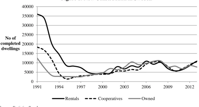
Figure 1 illustrates that construction of new dwellings decreased during the early 1990s, mainly due to decreased construction of rented dwellings. Several factors contributed to low levels of new construction onwards: 1) there was an economic recession between 1992 and 1998, 2) real interest rates increased, 3) the government raised VAT on new construction, 4) abrogated interest rate subsidies on new construction of rentals, and 5) reduced interest deductions on mortgage loans (National Housing Credit Guarantee Board, 2011). Despite low levels of new construction, the national average of housing per capita was almost constant between 1990 and 2012.8 However, there are considerable regional variations. Figure 2 illustrates how the number of “living-space-equivalent”9_{dwellings per capita developed between 1990 and 2012. In the three metropolitan}

commuting areas (Stockholm, Gothenburg and Malmö), the number of living-space-equivalent dwellings per capita was lower in 2012 compared to the early 1990s. However, outside the metropolitan areas the number of dwellings per capita had increased.

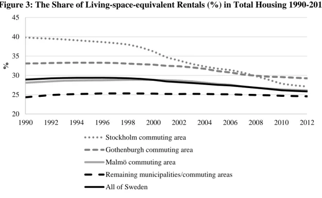
Figure 3 illustrates how the share of rentals in total living space has changed since 1990. At the national level, the share of rentals fell from about 29 to 26 percent between 1990 and 2012, which was entirely driven by the metropolitan areas. Both the decline in new construction and the

7_{For example, the share of the population in Sweden residing in “good housing standards” was 91.8 percent in 2009. The average}

for EU27 was 77.8 percent. Also, the share of individuals between 20 and 34 years of age still living with their parents was 18.5 percent in 2008. The average for EU27 was 45.8 percent. (Statistics Sweden, 2011).

8_{We stop at 2012 because there is a break in the data between 2012 and 2013.}

9_{We used tenure average size for the period 2006-2012 and assigned the following weights: Owned dwellings=1, Cooperative}

housing=0.548, Rentals=0.513. Average size (in square metres) is not available back to 1990 and available data is based on a random selection of dwellings. We therefore use average tenure size from the samples between 2006 and 2012 to determine the weights. (Source: Statistics Sweden , www.scb.se)

(5)

Figure 1: New Construction in Sweden

Source: Statistics Sweden

considerable number of tenure conversions contributed to the decrease in rentals. Between 1991 and 2012, there were about 170,000 tenure conversions (125,000 in Greater Stockholm alone).10

In sum, the developments during the past two decades until 2012 appear undramatic when observing national level data. However, geographical differences may have affected mobility.

Figure 2: Living-space Equivalent Number of Dwellings Per Capita 1990-2012

10_{Author’s calculations, Statistics Sweden.}

0 5000 10000 15000 20000 25000 30000 35000 40000 1991 1994 1997 2000 2003 2006 2009 2012 No of completed dwellings

Rentals Cooperatives Owned

0.28 0.29 0.3 0.31 0.32 0.33 0.34 0.35 0.36 0.37 0.38 1990 1992 1994 1996 1998 2000 2002 2004 2006 2008 2010 2012 Stockholm commuting area Gothenburgh commuting area

Malmö commuting area Remaining municipalities/commuting areas All of Sweden

(6)

Figure 3: The Share of Living-space-equivalent Rentals (%) in Total Housing 1990-2012

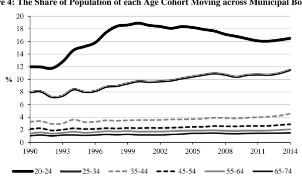
Figure 4 illustrates the share of individuals for different age cohorts that moved between municipalities each year between 1990 and 2014. The intermunicipal migration rate of individuals in the 20– 24 age group has decreased after peaking in 2000, but has increased or remained constant for all the remaining age cohorts.

4. METHODOLOGY AND DATA 4.1 The Model

The data is from Statistics Sweden. The model is a modified gravity model that estimates intermunicipal migration flows as a function of push and pull factors at the destination and the origin. There are numerous papers about interregional migration that estimate different versions of gravity models. Some model the number of migrants (Peeters, 2012; Piras, 2017) and some model migration in relation to the population at the origin or destination (Maza & Villaverde, 2004; Sousa, 2014). The current paper belongs to the latter strand.

Migration data was sorted by origin, destination, and age.11 For confidentiality reasons, migrants were divided into the following age cohorts: 20‒24, 25‒34, 35‒44, 45‒54, 55‒64, and 65‒74. We focus on individuals in their productive age. There is a break in the data after 2012, as Statistics Sweden has revised their methods for collecting data on the number of dwellings after 2012 and consequently, we restrict our analysis to the period 1993-2012. We employ panel

11_{This was ordered specifically as it is not officially available at Statistics Sweden’s website. While the total number of in-migrants}

and out-migrants as well as their age are available, all migration flows sorted on origin and destination municipalities are not.

20 25 30 35 40 45 1990 1992 1994 1996 1998 2000 2002 2004 2006 2008 2010 2012 %

Stockholm commuting area Gothenburgh commuting area Malmö commuting area

Remaining municipalities/commuting areas All of Sweden

(7)

Figure 4: The Share of Population of each Age Cohort Moving across Municipal Borders

data containing annual observations at the municipal level and estimate the following equation: (1) ln �𝑚𝑚𝑚𝑚𝑚𝑚𝑧𝑧𝑧𝑧,𝑡𝑡

𝑎𝑎𝑎𝑎𝑎𝑎

𝑎𝑎𝑚𝑚𝑎𝑎_{𝑧𝑧,𝑡𝑡−1}𝑎𝑎𝑎𝑎𝑎𝑎 � = 𝛼𝛼 + 𝜇𝜇𝑧𝑧𝑧𝑧+ 𝜇𝜇𝑡𝑡+ 𝛽𝛽𝑧𝑧𝑋𝑋𝑧𝑧+ 𝛽𝛽𝑧𝑧𝑋𝑋𝑧𝑧+ 𝜀𝜀𝑧𝑧𝑧𝑧,𝑡𝑡

In Equation (1), 𝑚𝑚𝑚𝑚𝑚𝑚_{𝑧𝑧𝑧𝑧,𝑡𝑡}𝑎𝑎𝑚𝑚𝑎𝑎 is the number of individuals belonging to age cohort age (20‒24, 25‒34, 35‒44, 45‒54, 55‒64, 65‒74) that migrated from the origin (municipality w) to the destination (municipality z) during year t provided that the gross flows of migrants from w to z is positive. One “complication” is the absence of migration flows between some municipalities. We remove the zero elements by following the procedures of Smith Conway and Houtenville (2003),12

Sousa (2014),13 and Önder and Schlunk (2015). While there may be other approaches to dealing with this problem, they require identification of some variable that explains why migration between two municipalities is zero, but which at the same time does not explain the magnitude of migration rates when they are positive,14 which we argue to be unrealistic. Employing a censored regression in a panel data setting (e.g. a Tobit model) does not allow estimation of a fixed effects model as there is no unbiased estimator that allows the fixed effects to be conditioned out of the likelihood (Honoré, 1992).

𝑎𝑎𝑚𝑚𝑎𝑎_{𝑧𝑧,𝑡𝑡−1}𝑎𝑎𝑚𝑚𝑎𝑎 is the population of age cohort age at the destination at the end of the year prior to migration. Hence, the dependent variables in Equation (1) are the natural logarithms of the gross migration rates in z through in-migration from w. We use the natural logarithms because they can

12_{They modelled net migration and removed observation where the number of in-migrants equaled the number of out-migrants.} 13_{Santos Silva and Tenreyro (2006) find no effect of removing zeros in a poisson model. Observations with zero observations have}

predicted values that are close to zero. Removing the zeros means that our panels will become unbalanced, which is not a problem.

14_{A sample selection model could have been appropriate in that case.}

0 2 4 6 8 10 12 14 16 18 20 1990 1993 1996 1999 2002 2005 2008 2011 2014 % 20-24 25-34 35-44 45-54 55-64 65-74

(8)

make variables more normally distributed15 and because it facilitates comparing regression results between age cohorts as migration rates are higher for the younger than the older individuals.16 Any individual invariant time effect that are not included are controlled for by including year dummies (𝜇𝜇_𝑡𝑡). The idiosyncratic errors must be uncorrelated across individuals and time-specific effects that have symmetric effects on migration flows between all municipalities. Unexplained migration flows are in the residual (𝜀𝜀_{𝑧𝑧𝑧𝑧,𝑡𝑡t}). 𝜇𝜇_{𝑧𝑧𝑧𝑧} are pairwise fixed effects. We employ Driscoll-Kraay standard errors that are robust to heteroskedasticity, as well as general forms of serial and spatial autocorrelation. Although the consistency of Driscoll-Kraay’s correction relies on a large number of time periods, it has been found superior compared to OLS, White’s, Rogers, and Newey-West standard errors when cross-sectional dependence is present; even when the number of time periods is relatively small.17

We separate between short- and long-distance moves and estimate two models. Model 1 estimates intermunicipal migration within commuting regions18 (short-distance migration), and Model 2 estimates intermunicipal migration between commuting regions (long-distance migration). As mentioned earlier, previous research suggest that job opportunities and educational purposes may be relatively important in explaining long-distance migration, while housing considerations are more important for short-distance moves (Gleave & Cordey-Hayes, 1977; Widerstedt, 1998; Niedomysl, 2011). Although it is obvious that migration within commuting regions can be more long-distance than migration to/from the closest commuting area, “short” and “long” refers to additional aspects besides geographical distance. As discussed by Niedomysl (2011), an important factor is whether migrants will need to replace only some of or all the key places that they normally visit during a workweek (schools, daycare, work etc.).19 Migration between commuting areas will imply more total displacement than migration within commuting areas because the former is more likely to be associated with a job shift than the latter.

4.2 Variables

We are primarily interested in two things. How does the physical stock of housing and tenure distribution affect intermunicipal mobility of different age cohorts? We hypothesize that the housing stock correlates with housing supply and housing vacancies. Also, tenure distribution may affect mobility differently depending on the preferences of housing consumers and the stringency of the rent-regulation system.

To represent “housing characteristics, we include the number of used, living-spaced-equivalent dwellings per capita, new construction, and the shares of the housing stock and new dwellings that consist of rentals. We distinguish between used and new dwellings because they are not equally affordable. Also, a new dwelling always generates a minimum of one vacancy whereas new vacancies among existing dwellings arise due to specific events, such as deaths or out-migration/emigration.

15_{Even if we divide by population at the destination, the dependent variables are highly skewed before taking logs. Sousa (2014)}

models the log of the migration rate.

16_{The interpretation of coefficient estimates when taking logs will be the percentage change of gross migration rate due to a unit}

change of the explanatory variables.

17_{Hoechle (2007) performed Monte-Carlo simulations for different values of T (5<T<40). In this paper, T=20. We employ the}

xtscc command in Stata to obtain Driscoll-Kay’s standard errors.

18_{We employ Statistics Sweden standard of 2008; dividing all of Sweden’s 290 municipalities into 75 commuting areas.} 19_{Roseman (1971) separated between migration associated with “partial” or “total” displacement.}

(9)

Endogeneity may be a concern for various reasons. For instance, housing demand depends on per capita incomes, which are among the control variables. In addition, there is a potential for reverse causality because new dwellings may attract migrants, but new dwellings can also be an outcome of planned in-migration. However, we lack access to good instruments that vary between both municipalities and years.20 Hence, we choose the second best option and lag the explanatory variables instead.

We do not include housing prices because our model can be perceived as a reduced form regression that includes common demand and supply-side factors usually incorporated in empirical house price models (Hort, 1998; Oikarinen, 2012). First, we include housing variables that represent housing supply. Second, we include year dummies, which capture annual variations in mortgage interest rates because regional differences in mortgage interest rates are low. Third, we include per capita incomes and relative population that affect housing demand. Including house prices somewhat weakens the estimated impact of the housing market variables. 21_{We interpret}

this as evidence supporting the argument that the included housing market variables partially affect mobility through their effect on house prices.

We include a set of control variables that represent “economic opportunities” at the origin and destination. According to neoclassical theory, regions where per capita incomes are high and chances of employment are good should attract labor migrants (Sjaastad, 1962; Todaro, 1969; Harris and Todaro, 1970; Westerlund, 1997; Cushing and Poot, 2004 ). However, different patterns may be observed when analyzing aggregate data. An opposite effect can emerge because the same mechanisms that attract individuals also discourages people from leaving, which means that there will be fewer housing vacancies (this is also discussed by Piras, 2017).

Moreover, per capita income, the average level of human capital, and employment rates are all correlated and endogenous, and should not be included together. We therefore include per capita income and the lagged first differences of the municipal and commuting areas employment rates, because in-migration should be higher to regions where employment grows faster (Hämäläinen & Böckerman, 2004). Further, we include the share of employment enrolled in the primary sector (hunting, forestry, fishing and agriculture), which is negatively correlated to the average level of human capital. Also, we include municipal tax rates (TAX, OR_TAX). While high local taxes may discourage in-migration, the opposite effect may arise if they indicate a higher quality of local welfare services.

Further, individuals may base their choice to migrate on access to local amenities (e.g., supply of cultural activities, climate etc.) and on transaction costs of moving (approximated by the geographical distance between the origin and destination) (Greenwood, 2005). We do not have access to long time series data on amenities at the municipal level.22 Thus, our best solution is to include pairwise fixed effects in our panel (µzw). Pairwise fixed effects control for the effects of

distance between the origin and destination, and the effects of relative access to amenities that do not vary over time (for example, relative climate conditions).

20_{If data were available, one option could have been some measure of the stringency of local land-use regulations.} 21_{These results are available from the author upon request.}

(10)

Table 1: Description of Variables Variables with Prefix “OR” are Characteristics at Origin

Name of variable Description/Definition

DEPENDENT VARIABLE

._MIGAGE

Natural logarithm of migration rate of individuals in age cohort age (20‒24, 25‒34, 35‒44, 45‒54, 55‒ 64, 65‒74 during year t in municipality z through out-migration from municipality w.

HOUSING VARIABLES HOUSING

OR_HOUSING

The number of used “living-spaced-equivalent” dwellings per capita, i.e. the housing stock lagged by two years divided by the population lagged by one year. We lag the housing stock by two years because we separate between used dwellings and new construction (and the latter is lagged by one year). The following weights are used: owned dwelling=1; cooperative dwelling=0.548; rental=0.513. NEW_CONSTRUCTION

OR_NEW_CONSTRUCTION _{Lagged by one year. The following weights are used: owned dwelling=1; cooperative dwelling=0.548;}The number of completed living-spaced-equivalent dwellings through new construction per capita. rental=0.513. Lagged by one year.

RENTALS

OR_RENTALS The share of used living-spaced-equivalent rentals in the stock of housing. The housing stock is lagged _{by one year and the number of rentals are lagged by two years. We lag the number of rentals by two} years because we separate between used and new rentals (and new rentals are lagged one year (see

below). RENTALS_NEW

OR_RENTALS_NEW The share of living-spaced-equivalent rentals in new construction. Lagged by one year. ECONOMIC OPPURTUNITIES

∆EMPLOYMENT_REGION

OR_∆EMPLOYMENT_REGION _{the commuting are population 15-74 years of age (excluding the destination and origin municipalities).}The first difference of the commuting area employment rate (number of jobs in commuting divided by Lagged by one year

PRIMARY OR_PRIMARY

The share of all jobs in municipality in agriculture, hunting, fishing and forestry. ∆EMPLOYMENT

OR_∆EMPLOYMENT The first difference of the employment rate (number of jobs in municipality divided by the population _{15-74 years of age). Lagged by one year.} INCOME

OR_INCOME Natural logarithm of earned income divided by population 15 to 74 years of age. Lagged by one year. _{Earned income includes salaries, unemployment benefits, sick-leave benefits, parental benefits and} pensions (in thousands of SEK).

TAX

OR_TAX Municipal tax rate.

OTHER POPage_{/OR_POP}age

The population of age cohort age at the destination relative to the population of age cohort age at the origin. Lagged by one year.

DEATHS

OR_DEATHS Number of deaths per capita.

FOREIGN

OR_FOREIGN The share of foreign citizens. Lagged by one year.

Source: Statistics Sweden.

Also, we include demographic factors. We expect positive/negative relationships between the death rates at the destination/origin with migration because deaths generate housing vacancies. The share of foreign born at the origin and destination could affect migration in several ways. A tendency of “white flight” would reduce in-migration and increase out-migration to municipalities when the share of foreign-born increases.

(11)

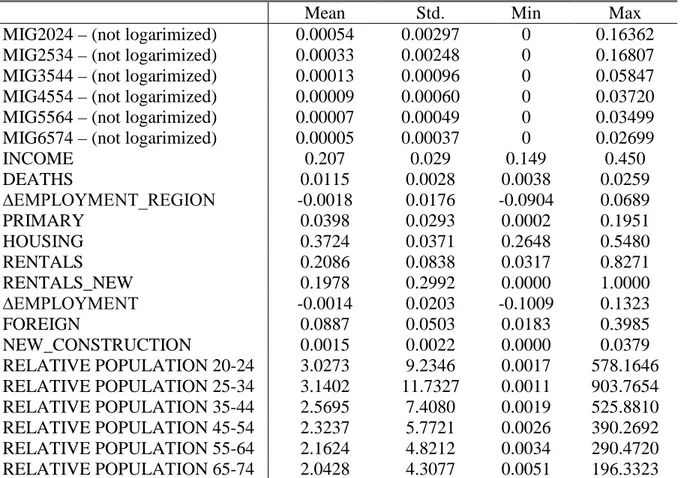
Table 2: Descriptive Statistics

Mean Std. Min Max

MIG2024 – (not logarimized) 0.00054 0.00297 0 0.16362 MIG2534 – (not logarimized) 0.00033 0.00248 0 0.16807 MIG3544 – (not logarimized) 0.00013 0.00096 0 0.05847 MIG4554 – (not logarimized) 0.00009 0.00060 0 0.03720 MIG5564 – (not logarimized) 0.00007 0.00049 0 0.03499 MIG6574 – (not logarimized) 0.00005 0.00037 0 0.02699

INCOME 0.207 0.029 0.149 0.450 DEATHS 0.0115 0.0028 0.0038 0.0259 ∆EMPLOYMENT_REGION -0.0018 0.0176 -0.0904 0.0689 PRIMARY 0.0398 0.0293 0.0002 0.1951 HOUSING 0.3724 0.0371 0.2648 0.5480 RENTALS 0.2086 0.0838 0.0317 0.8271 RENTALS_NEW 0.1978 0.2992 0.0000 1.0000 ∆EMPLOYMENT -0.0014 0.0203 -0.1009 0.1323 FOREIGN 0.0887 0.0503 0.0183 0.3985 NEW_CONSTRUCTION 0.0015 0.0022 0.0000 0.0379 RELATIVE POPULATION 20-24 3.0273 9.2346 0.0017 578.1646 RELATIVE POPULATION 25-34 3.1402 11.7327 0.0011 903.7654 RELATIVE POPULATION 35-44 2.5695 7.4080 0.0019 525.8810 RELATIVE POPULATION 45-54 2.3237 5.7721 0.0026 390.2692 RELATIVE POPULATION 55-64 2.1624 4.8212 0.0034 290.4720 RELATIVE POPULATION 65-74 2.0428 4.3077 0.0051 196.3323 Source: Statistics Sweden. Shares are decimals, not percentages. Note that averages of the explanatory variables refer to all municipalities (although zero elements of migration were removes in the regressions).

We include the population of the current age cohort at the destination divided by the population at the origin in order to investigate the role of population size. Except for population, we do not include the explanatory variables expressed as ratios between the origin and the destination. This is done so that we do not force “symmetry” on the model, meaning that migrants must respond similarly to identical changes in explanatory variables at the origin and the destination (Ghatak, Mulhern, & Watson, 2008). Table 1 contains a description of all variables. Summary statistics are presented in Table 2.

5. EMPIRICAL RESULTS 5.1 Regression Results

Tables 3 and 4 show the results where we have separated between intermunicipal migration within commuting regions (short migration) and between commuting regions (long migration), respectively. Variables with the prefix “OR” represent characteristics at the origin municipalities while remaining variables are destination characteristics.

The control variables are (when significant) in line with expectations. However, regression results for the income and labor market variables (INCOME, OR_INCOME, OR_PRIMARY, PRIMARY, ∆EMPLOMENT_REGION, ∆EMPLOMENT, ∆EMPLOMENT_REGION, ∆OR_EMPLOMENT ,∆OR_EMPLOMENT) are not consistent through all regressions. In the

(12)

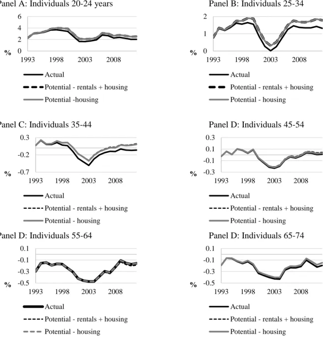
Table 3: Results Estimating Short-distance Migration (Intermunicipal Migration within Commuting Regions)

Dependent variables

Independent variables MIG2024 MIG2534 MIG3544 MIG4554 MIG5564 MIG6574

HOUSING 1.406*** (0.007) 3.340*** (0.000) 3.952*** (0.000) 1.149 (0.136) -1.095 (0.271) 3.044*** (0.000) NEW_CONSTRUCTION 3.061*** (0.005) 5.519*** (0.001) 4.924** (0.014) 8.000*** (0.000) 4.152** (0.013) 4.461 (0.187) RENTALS 0.447*** (0.002) -0.123 (0.209) -0.337** (0.033) 0.0797 (0.662) -0.407 (0.115) -1.270*** (0.001) RENTALS_NEW 0.0168* (0.090) -0.000890 (0.947) 0.0114 (0.319) 0.00655 (0.626) -0.0190 (0.405) 0.000435 (0.975) FOREIGN -1.466*** (0.008) -1.835*** (0.000) 1.310* (0.061) -0.524 (0.300) -0.856** (0.029) 1.076* (0.065) DEATHS 9.530* (0.095) 5.713 (0.305) 5.478 (0.112) -3.082 (0.645) -7.371* (0.072) -25.67** (0.015) INCOME -0.908*** (0.000) -1.284*** (0.000) -0.803*** (0.002) -0.965*** (0.000) -1.287*** (0.000) -0.441** (0.025) ∆EMPLOMENT -0.0488 _(0.828) -0.0990 _(0.626) -0.352* _(0.064) _(0.124)-0.438 _(0.709)0.179 _(0.642)0.200 PRIMARY SECTOR -0.202 (0.528) -0.856 (0.114) -1.134* (0.086) 0.365 (0.464) -0.770 (0.216) -0.923 (0.183) TAX -1.757*** (0.008) -1.310* (0.072) -1.865** (0.012) -0.774 (0.319) 0.263 (0.770) -2.640*** (0.008) OR_HOUSING -1.544** (0.042) -2.401** (0.028) -0.870 (0.170) 0.476 (0.386) 1.759*** (0.000) 2.225*** (0.000) OR_NEW_CONSTRUCTION -0.485 (0.609) -2.794* (0.058) -1.380 (0.146) -0.159 (0.912) -2.902** (0.046) -3.393* (0.079) OR_RENTALS 0.172 (0.183) -0.0587 (0.773) -0.405** (0.011) 0.0270 (0.851) 0.535** (0.017) 1.114*** (0.001) OR_RENTALS_NEW 0.0124 (0.318) 0.0111 (0.325) 0.0129 (0.372) 0.00861 (0.339) -0.00643 (0.526) 0.0194 (0.246) OR_FOREIGN -0.587 (0.291) 2.617*** (0.000) 1.959*** (0.002) 1.332** (0.028) 1.487* (0.053) -0.0629 (0.908) OR_DEATHS 0.472 (0.818) -8.980** (0.017) -3.792 (0.144) -8.254*** (0.001) -8.411* (0.065) -2.535 (0.616) OR_INCOME -0.648*** (0.000) 0.386 (0.181) -0.230 (0.333) -0.1000 (0.699) 0.138 (0.468) -0.228 (0.463) ∆OR_EMPLOYMENT 0.354 (0.108) 0.290 (0.256) 0.336** (0.017) -0.122 (0.581) -0.343* (0.100) -0.397 (0.250) OR_PRIMARY_SECTOR -0.0725 (0.819) 2.080*** (0.000) 1.547*** (0.007) -0.553* (0.075) 0.253 (0.438) -0.174 (0.783) OR_TAX -0.0253 (0.975) -0.130 (0.923) 0.0707 (0.915) 0.560 (0.404) -1.394** (0.037) -1.328 (0.353)

POPage_{/OR_POP}age -0.0260***

(0.000) -0.0141*** (0.000) -0.0328*** (0.000) -0.0391*** (0.000) -0.0326*** (0.000) -0.0137*** (0.003) N 40746 43670 39722 36933 32360 25291 ADJUSTED R2 _0.894 _0.898 _0.861 _0.846 _0.813 _0.770 AKAIKE 46046.2 52841.3 52346.7 48352.2 44599.5 35593.6 SCHWARZ 46399.4 53197.4 52698.9 48701.4 44943.2 35927.3 FIXED INDIVIDUAL

EFFECTS YES YES YES YES YES YES

FIXED PERIOD EFFECTS YES YES YES YES YES YES

Source: Author’s estimations. *p<0.1 **p<0.05 ***p<0.0101.There are 290 municipalities in Sweden. However, due to previous “township splitting” eight municipalities was merged to form four: Knivsta+Uppsala, Nykvarn+Södertälje, and Borås+Bollebygd, Örebro+Lekeberg. Fixed effects are not reported. P-values of 2-sided hypotheses are in parenthesis.

(13)

Table 4: Results Estimating Long Distance Migration (Intermunicipal Migration between Commuting Regions)

Dependent variables

Independent variables MIG2024 MIG2534 MIG3544 MIG4554 MIG5564 MIG6574

HOUSING 1.695*** (0.001) 2.891*** (0.000) 5.238*** (0.000) 1.293*** (0.000) 0.0264 (0.948) 2.502*** (0.000) NEW_CONSTRUCTION -0.948 (0.524) -2.335 (0.353) 0.892 (0.588) 0.375 (0.649) -1.552 (0.374) 3.504* (0.095) RENTALS 0.000345 (0.997) 0.0428 (0.784) -0.250*** (0.001) 0.00915 (0.900) -0.625*** (0.000) -0.905*** (0.000) RENTALS_NEW 0.00699 (0.313) 0.00532 (0.378) -0.00869 (0.229) -0.00387 (0.445) -0.0180** (0.015) -0.0190** (0.027) FOREIGN -0.743** (0.043) -3.741*** (0.000) -1.155*** (0.001) -1.549*** (0.000) -1.168*** (0.000) 1.473*** (0.002) DEATHS 5.965** (0.047) 7.828** (0.010) 2.883 (0.201) 5.176** (0.014) -0.510 (0.771) -8.866** (0.025) INCOME -0.155 (0.443) -0.735*** (0.001) -0.518*** (0.000) -0.296*** (0.001) -1.053*** (0.000) -0.613*** (0.000) ∆EMPLOMENT_REGION 0.323 (0.131) 0.280 (0.136) -0.179 (0.506) 0.0394 (0.766) -0.681** (0.043) -0.197 (0.698) PRIMARY SECTOR 0.531 (0.272) 0.749 (0.126) -0.0375 (0.939) 1.136*** (0.000) 0.117 (0.740) -0.139 (0.785) TAX -1.688** (0.026) -2.897*** (0.000) -3.844*** (0.000) -0.845** (0.038) -2.959*** (0.000) -2.971*** (0.000) OR_HOUSING -2.698*** (0.002) -3.324*** (0.001) -2.167*** (0.000) -0.340 (0.161) -0.326 (0.381) 0.683 (0.225) OR_NEW_CONSTRUCTION -0.957 (0.429) 0.903 (0.671) 0.367 (0.530) -0.608 (0.547) 1.467 (0.361) -1.965 (0.243) OR_RENTALS 0.352 (0.119) 0.316 (0.120) -0.482*** (0.000) -0.226* (0.098) 0.127 (0.563) -0.0368 (0.625) OR_RENTALS_NEW 0.0180 (0.179) 0.00516 (0.679) 0.0116** (0.017) -0.00631 (0.366) -0.00464 (0.456) 0.00458 (0.567) OR_FOREIGN 0.433 (0.125) 1.828*** (0.000) 1.751*** (0.000) 0.825*** (0.003) 1.157*** (0.000) 0.578* (0.073) OR_DEATHS -6.468** (0.017) -13.96*** (0.000) -4.413*** (0.009) -3.252** (0.026) -4.125** (0.047) -2.936** (0.030) OR_INCOME -0.421 (0.140) -0.144 (0.626) 0.249** (0.045) 0.0868 (0.359) 0.348** (0.016) 0.522*** (0.000) ∆OR_EMPLOYMENT_REGION -0.425** _(0.024) -0.434** _(0.036) -0.0909 _(0.774) _(0.469)-0.101 -0.394* _(0.089) -0.0601 _(0.719) OR_PRIMARY_SECTOR 0.321 (0.175) 0.436 (0.200) 0.700 (0.102) -0.506* (0.076) 0.205 (0.494) 0.541*** (0.009) OR_TAX 0.830* (0.080) 0.218 (0.795) 1.092* (0.086) 0.671** (0.021) 0.255 (0.577) 0.880** (0.034) POPage_{/OR_POP}age

-0.00816*** (0.000) -0.00268*** (0.000) -0.00374** (0.011) -0.00946*** (0.000) -0.0149*** (0.000) -0.0184*** (0.000) CONSTANT -7.701*** (0.000) -8.256*** (0.000) -8.637*** (0.000) -8.660*** (0.000) -7.923*** (0.000) -8.214*** (0.000) N 305649 292114 174558 131521 101287 71030 ADJUSTED R2 _0.847 _0.850 _0.839 _0.850 _0.845 _0.837 AKAIKE 329530.2 332126.4 168672.2 105704.0 77975.5 46812.3 SCHWARZ 329966.0 332560.4 169085.1 106105.3 78366.1 47188.3

FIXED INDIVIDUAL EFFECTS YES YES YES YES YES YES

FIXED PERIOD EFFECTS YES YES YES YES YES YES

Source: Author’s estimations. *p<0.1 **p<0.05 ***p<0.0101.There are 290 municipalities in Sweden. However, due to previous “township splitting” eight municipalities was merged to form four: Knivsta+Uppsala, Nykvarn+Södertälje, and Borås+Bollebygd, Örebro+Lekeberg. Fixed effects are not reported. P-values of 2-sided hypotheses are in parenthesis.

(14)

Swedish context, several studies have found that regional differences in employment opportunities have a larger impact on migration flows than regional wage differences (Dahlberg & Holmlund,1978; Westerlund, 1997; Fredriksson, 1999; Aronsson, Lundberg, & Wikström, 2001). Also, as discussed above, the same mechanisms that attract individuals can prevent people from leaving. Previous studies find mixed results regarding the relationship between human capital at origin and destination areas and internal migration in e.g. Germany, Spain, and Italy ( Maza & Villaverde, 2004;Maza, 2006; Mitze & Reinkowski, 2011; Piras, 2017).

In line with expectations, ∆OR_EMPLOYMENT_REGION is negative for the 20-24 and 25-34 age cohorts when modeling long-distance migration. Also, ∆_EMPLOYMENT_REGION is positive and almost significant (p-values are around 0.13) for the 20-34 age cohorts. But, the employment variables are insignificant or with the “wrong” sign for the remaining age cohorts.23Overall though, the results suggest that job market considerations are more important for long-distance moves than for short-distance moves (as discussed above) and for younger adults than for older adults, which is in line with previous research (Hansen and Niedomysl, 2011; Mitze and Reinkowski 2011).

Another factor that may contribute to the inconsistency of our results is that we model intermunicipal migration. Previous studies on internal migration in Sweden have typically employed larger spatial units than municipalities e.g. counties (Westerlund, 1997; Gärtner, 2014). FOREIGN and OR_FOREIGN are mainly negative and positive, suggesting the presence of white flight. TAX and OR_TAX are, when significant, consistently negative and positive in both Tables 3 and 4, confirming the existence of economic reasons to move. As expected, DEATHS and OR_DEATHS are significantly positive and negative for the younger age cohorts because the occurrence of deaths generate housing vacancies, but DEATHS is negative for the 55-74 cohorts. This may reflect that municipalities with high death rates have a more constrained situation regarding care-taking of old people, because the death rate should be correlated with the share of elderly. Thus, the older segment of the workforce may prefer to move to places where the average age is relatively low. Also, recall that we model migration rates in relation to the actual population of the actual age cohorts at the destination, and municipalities with many and/or a high share of old people must attract many old in-migrants in order to obtain high in-migration rates. Finally, POPage_/ORPOPage_{is always negative and significant, confirming that larger municipalities have}

larger outflows of migrants.

Turning to the housing variables, a larger stock of used dwellings per capita at the destination (HOUSING) appears to attract migrants from other commuting regions as well as from other municipalities from the same commuting region. Coefficient estimates are generally stronger in Table 3, which is in line with previous studies that have found that housing considerations are more important for short than long-distance moves. NEW CONSTRUCTION displays a similar pattern and is positive and significant for all five age cohorts in Table 3 (short-distance migration) but only for one age cohort (65-74) in Table 4. Possibly, a larger variability of house prices between than within commuting regions implies that “urban newcomers” may not afford new dwellings when moving to the metropolitan areas. Even if they were homeowners before migrating, the value of a previous house may not be enough to cover the down payment for a new house in a more expensive area, which forces them to consider used dwellings instead. Because

23_{In alternative regressions, we remove the employment variables. This has little impact on remaining coefficient estimates. These}

(15)

young adults have low average incomes, one could carefully interpret the results as evidence for vacancy chains that liberalize dwellings, which are relatively affordable,24 However, the estimated coefficients also suggest that NEW CONSTRUCTION stimulates mobility relatively little for the 20-24 age cohort, indicating that new dwellings are relatively unavailable for the youngest adults.

Further, OR_HOUSING is negative and significant for two and three age cohorts in Tables 3 and 4, respectively. This in line with previous research that has found that spacious living reduces incentives to move and that over-crowded households are more mobile than are others (Aquilino, 1990: De Jong et al., 1991). Similarly, OR_NEW_CONSTRUCTION is negative and significant for three age cohorts in Table 3 but always insignificant in Table 4, which again suggest that housing considerations are more important for short- than for long-distance moves.

Regarding the 55-64 and 65-74 age cohorts, their mobility patterns are different compared to the other age cohorts between 20 and 54 because the number of out-migrants from the metropolitan areas is considerably higher than the number of in. Arguably, they are moving from bigger to smaller dwellings to a larger extent than younger adults because they may be leaving their house once their children have left the nest. This may explain why NEW_CONSTRUCTION is only significant for the 65-74 age cohort in Table 4. Also, the fact that OR_HOUSING is positive for the 55-74 age cohorts in Table 3 may reflect that their mobility patterns differ in comparison to other age groups.

An objective of this paper is to investigate whether the decreased share of rentals in the metropolitan areas has affected mobility. Generally, mobility is higher in the rented sector than in the owned segment of the housing market, which is often explained by comparably low transaction costs of moving. However, the effects of changes in tenure distribution on the intermunicipal migration not only depends on the costs of moving, but also on the supply of rentals relative to owned housing and on consumer tenure preferences. When significant, the results suggest a negative impact of an increased share of rented dwellings at the destination (RENTALS) for most age cohorts. In general, effects appear stronger on mobility within than between commuting regions. Further, the share of rentals in new construction (RENTALS_NEW) is predominantly negative (although rarely significant). In sum, these results support a general preference for owned housing over rented dwellings, which has also be proven to the case in several surveys (Swedish National Board of Housing, Building and Planning, 2014).

Further, OR_RENTALS is negative for some age cohorts and positive for some. These results do not support that rental-housing tenants are necessarily more mobile than home owners, or that an increased share of rentals stimulates intermunicipal mobility in general. As mentioned previously, turnover rates are higher among rented dwellings than among owned. Consequently, the results may indicate that the higher turnover rate of rented housing is explained by the overrepresentation of young people and non-natives rather than by low transaction costs for moving. However, for the 20-24 age cohort results are more in line with expectations and increasing the share of rentals at the destination (in both used dwellings and in in new construction) appear to stimulate in-migration. This is not surprising considering that young adults are over-represented in the rented sector.

5.2 How have Housing Market Developments Affected Intermunicipal Mobility?

(16)

Now, we estimate the potential magnitude of intermunicipal migration if housing per capita (HOUSING, OR_HOUSING) and the share of rentals in total housing (RENTALS, OR_RENTALS, NEW_RENTALS, OR_NEW_RENTALS) had remained at the level of 1992, and if new construction (NEW_CONSTRUCTION, OR_NEW_CONSTRUCTION) had matched actual population growth each year. Considering that some results were not consistent when comparing age cohorts, it is interesting to investigate if this translates into meaningful differences when simulating the effects of actual changes since 1992. In a Swedish context, the policy debate has been focused on the need to increase new construction in general and the stock of relatively cheap dwellings in particular. This simulation exercise is a contribution to that debate.

We cannot rule out that insignificant variables have zero effect and coefficients were thus set to zero for variables that were not significant (at least at the ten percent level). In general, the regression results suggest that low levels of new construction negatively affect short-distance migration stronger that long-distance migration. This is confirmed by simulations that suggest (not presented here) that changes since 1992 have had a stronger impact on mobility within commuting regions than between (recall that migration is more strongly related to new construction and share of rentals in Table 3 than 4). However, we are choosing a careful approach, thereby not presenting the results for single municipalities because regression results represent average relationships.

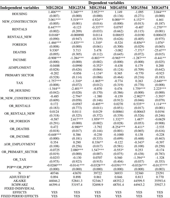
Instead, Figures 5-10 illustrate the actual and potential share of intermunicipal migrants for each age cohort migration annually between 1993 and 2012. We separate the isolated effects of housing per capita changes and the joint effect of changes in housing per capita and the share of rentals. We separate between intermunicipal migration within (short-distance) and between commuting (long-distance) areas. If the black-spotted and grey-spotted-lines are above/below the solid black-line, this means that housing market developments since 1992 have negative/positively affected intermunicipal mobility.

In general, the estimated effects of housing per capita changes and tenure distribution since 1992 on intermunicipal migration are weak, although a tendency that housing per capita changes have started to generate stronger negative effects in recent years can be spotted. The simulations indicate that the strongest effect are on intermunicipal migration for young adults between 20 and 24 years of age within commuting regions (Figure 5 Panel B). Most of the effects steam from the changes in tenure distribution and not from housing per capita changes. For the other age cohorts, the results generally indicate that changes in tenure distribution have no or a weakly positive effect on mobility (the 55-64 age cohort is an exception). As discussed above, this supports a preference for owned housing. Further, for remaining age cohorts, the effects of housing per capita changes are generally weak but negative on short- as well as on long-distance migration, although results are not all consistent through all age cohorts. The simulations indicate a positive effect of housing per capita changes on the mobility of the 35-44 age cohort (long-distance migration, Figure 7 Panel A) and 65-74 age cohort (both short- and long-distance migration, Figure 10). Technically, this is because the absolute value of HOUSING is larger than the corresponding value of OR_HOUSING and that OR_HOUSING is positive for the 65-74 age cohort in Table 4. Regarding the 65-74 age cohort, their mobility patterns are different compared to the younger cohorts as they have negative net migration to the metropolitan areas. Thus, the results may reflect that the older segment of the workforce have benefitted from recent housing market developments because they are leaving the metropolitan areas and moving to areas where housing is cheaper and more available.

(17)

Figure 5: Comparison of Actual and Potential Internal Migration Rates (%) for Individuals between 20 and 24

Panel A: Between Commuting Regions Panel B: Within Commuting Regions

6 8 10 12 14 1993 1998 2003 2008 % Actual Potential - total Potential - Housing 5.5 6 6.5 7 1993 1998 2003 2008 % Actual Potential - total Potential - Housing 3 4 5 6 1993 1998 2003 2008 % Actual Potential - total Potential - Housing 3.5 4 4.5 5 5.5 1993 1998 2003 2008 % Actual Potential - total Potential - Housing 1.2 1.7 2.2 1993 1998 2003 2008 % Actual Potential - total Potential - Housing 1.5 2 2.5 3 1993 1998 2003 2008 % Actual Potential - total Potential - Housing

(18)

0.8 0.9 1 1.1 1993 1998 2003 2008 % Actual Potential - total Potential - Housing 1 1.2 1.4 1.6 1993 1998 2003 2008 % Actual Potential - total Potential - Housing 0.7 0.75 0.8 0.85 0.9 1993 1998 2003 2008 % Actual Potential - total Potential - Housing 0.6 0.8 1 1.2 1993 1998 2003 2008 % Actual Potential - total Potential - Housing 0.5 0.6 0.7 0.8 1993 1998 2003 2008 % Actual Potential - total Potential - Housing 0.5 0.6 0.7 0.8 1993 1998 2003 2008 % Actual Potential - total Potential - Housing

(19)

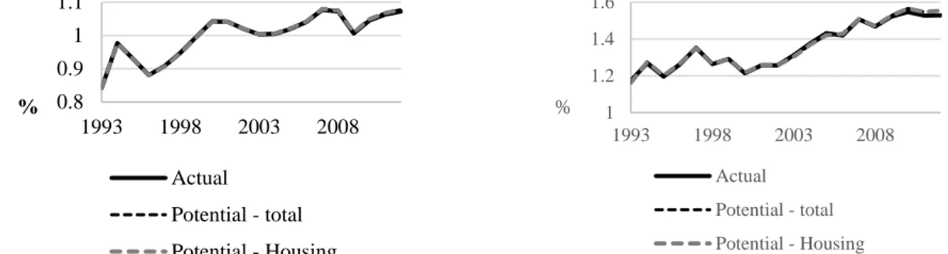
Figure 11: Actual and Potential Net Migration Rates to Stockholm Commuting Area

Panel A: Individuals 20-24 years Panel B: Individuals 25-34

Panel C: Individuals 35-44 Panel D: Individuals 45-54

Panel D: Individuals 55-64 Panel D: Individuals 65-74

In sum, although some of the estimated effects differ between age cohorts in terms of direction, they generally indicate weak effects on total intermunicipal mobility of housing market developments since 1992. However, effects are somewhat stronger for the 20-24 age cohort, which is primarily driven by the decreased share of rentals in the metropolitan areas.

However, simulating the effects at the national level can be misleading and ignores the regional dimension. Recall from Figures 2 and 3 that housing per capita and the share of rentals have decreased in the metropolitan areas while remaining almost constant in other regions. We therefore simulate the effects of housing market developments since 1992 on net migration to the metropolitan areas. We choose to focus on one region, the Stockholm commuting area in Figure 11. The simulations suggest that decreasing housing per capita has negatively affected net

0 2 4 6 1993 1998 2003 2008 % Actual

Potential - rentals + housing Potential -housing 0 1 2 1993 1998 2003 2008 % Actual

Potential - rentals + housing Potential - housing -0.7 -0.2 0.3 1993 1998 2003 2008 % Actual

Potential - rentals + housing Potential - housing -0.3 -0.1 0.1 0.3 1993 1998 2003 2008 % Actual

Potential - rentals + housing Potential - housing -0.5 -0.3 -0.1 0.1 1993 1998 2003 2008 % Actual

Potential - rentals + housing Potential - housing

(20)

migration to the Stockholm commuting area for all age groups except for the 55-64 cohort (coefficient estimates were insignificant in Table 3). The effects are strong in comparison to the estimated effects on intermunicipal migration for the whole country. Also, the effects are stronger for those who are relatively mobile, i.e. for young adults between 20 and 44 years of age. Changes in tenure distribution have had a small or no effect for all age cohorts.

6. CONCLUSIONS

The results in this paper suggest that while housing market developments in Sweden since the early 1990s have only weakly affected intermunicipal mobility at the national level, there are relatively strong negative effects on net migration to the metropolitan areas. In general, the results suggest that low levels of new construction negatively affects short-distance migration more than long-distance migration. But for the metropolitan areas, there are considerable negative effects on net migration from other regions too, because new construction has not kept pace with population growth in these regions. The effects are stronger for young adults (20-44) compared to the older adults (45-74). From this perspective, the results indicate that low levels of new construction is harmful for economic growth, because labor migration is typically associated with long-distance migration and because labor market related reasons to migrate have been found to be more important among young migrants. Further, the decreased share of rentals in the metropolitan areas appear to have negatively affected short-distance mobility of the youngest adults (20-24), but we did not find any evidence that it has affected mobility between commuting regions. However, this indicates that the strained situation on the rental market has affected the youngest adults more than others.

In sum, the current urbanization process would have taken place at an even faster pace, had the housing market developed differently. While we needed to limit our period to the years between 1993 and 2012, recent developments have shown that the levels of new construction have not matched population growth after 2012, particularly in metropolitan areas. The amount of municipalities that have declared they have a general housing shortage has continued to increase after 2012.25

On the positive side, we found that that new construction stimulates mobility for all age cohorts (short-distance migration in particular). Although new dwellings are unaffordable for some, they always offer at least one new vacancy which allows the formation of new households. In addition, new dwellings initiate vacancy that can liberate dwellings that are affordable for households at the lower end of the income spectrum. However, the estimated relationship is weaker for the youngest adults, which indicates a need for more variation in new construction in order to satisfy different needs, which may warrant housing policy interventions that are aimed at households with low incomes.

An interesting observation is that some variables (mainly housing and labor market related variables) were not all consistent and did not display the same sign for all age cohorts. While this may cast some doubt on the results, it also indicates a need for researchers to separate between different ages when studying determinants of internal migration and to come up with different setups of explanatory variables that vary with migrants age. In this paper, we have attempted to augment previous research and have analyzed the relationship between housing and internal

(21)

migration from a broad geographical perspective. However, for reasons of data availability we did not look into factors that explain migration within municipalities, which would be highly relevant.

REFERENCES

Abramsson, Marianne, Urban Fransson, and Lars-Erik Borgegård. (2004) “The First Years as Independent Actors in the Housing Market: Young Households in a Swedish Municipality,” Journal of Housing and the Built Environment, 19, 145–168.

Andersson, Roger and Lena Magnusson Turner. (2008) “Socioekonomiska och Demografiska Konsekvenser av Ombildningen av Hyresrätter till Bostadsrätter i Stockholms Stad 1995 – 2004 (Socioeconomic and Demographic Consequences of Tenure Conversions from Rentals to Cooperatives in Stockholm City 1995-2004),” Report to the Swedish Union of

tenants, last accessed November 2017 at

https://hgfhaninge.files.wordpress.com/2012/09/rapport_ombildningens_konsekvenser.pd f

Aquilino, William S. (1990) “The Likelihood of Parent-child Co-residence: Effects of Family Structure and Parental Characteristics,” Journal of Marriage and the Family, 52, 405–419. Aronsson, Thomas, Johan Lundberg, and Magnus Wikström. (2001) “Regional Income Growth

and Net Migration in Sweden, 1970–1995,” Regional Studies, 35, 823–830.

Ashby, Nathan J. (2007) “Economic Freedom and Migration between U.S. States,” Southern

Economic Journal, 73, 677–697.

Bloze, Gintautas. (2009) “Interregional Migration and Housing Structure in the East European Transition Country: A View of Lithuania 2001-2008,” Baltic Journal of Economics, 9, 47– 66.

Clark, William A.V. and Frans M. Dieleman. (1996) Households and Housing. Choice and

Outcomes in the Housing Market, 1st ed, N.J.: Center for Urban Policy Research, New Brunswick.

Conway, Karen S. and Andrew Houtenville, (2003) “Out with the Old, in with the Old. A Closer Look and Younger Versus Older Elderly Migration,” Social Science Quarterly, 84, 309– 328.

Cunningham, Christopher R. and Gary V. Engelhardt. (2008) “Housing Capital-gains Taxation and Homeowner Mobility: Evidence from the Taxpayer Relief Act of 1997,” Journal of

Urban Economics, 63, 803–815.

Cushing, Brian and Jacques Poot. (2004) “Crossing Boundaries and Borders: Regional Science Advances in Migration Modelling,” Papers in Regional Science, 83, 317–338.

Dahlberg, Åke and Bertil Holmlund. (1978) “The Interaction of Migration, Income and Employment in Sweden,” Demography, 15, 259–266.

Gierveld, Jenny De Jong, Aaart. C. Liefbroer and Erik Beekink. (1991) “The Effect of Parental Resources on Patterns of Leaving Home Among Young Adults in the Netherlands,”

European Sociological Review, 7, 55–71.

Dieleman, Frans M. (2001) “Modelling Residential Mobility: A Review of Recent Trends in Research,” Journal of Housing and Built Environment, 16, 249–265.

(22)

Engelhardt, Gary V. (2003) “Nominal Loss Aversion, Housing Equity Constraints, and Housing Mobility: Evidence from the United States,” Journal of Urban Economics, 53, 171–195. Emmi, Philip C. and Lena Magnusson. (1995) “Further Evidence on the Accuracy of Residential

Vacancy Chain Models,” Urban Studies, 32, 1361–1367.

Ermisch, John and Elizabeth Washbrook. (2012) “Residential Mobility: Wealth, Demographic and Housing Market Effects,” Scottish Journal of Political Economy, 59, 483–489.

Findlay, Allan and Robert Rogerson. (1993) “Migration, Places and Quality of Life: Voting with their Feet?'” in Tony Champion, ed., Population Matters. Paul Chapman Publishing Ltd: London, pp. 33–49.

Ferreira, Fernando, Joseph Gyourko, and Joseph, Tracy. (2010) “Housing Busts and Household Mobility,” Journal of Urban Economics, 68, 34–45.

Fredriksson, Peter. (1999) “The Dynamics of Regional Labour Markets and Active Labour Market Policy: Swedish Evidence,” Oxford Economic Papers, 51, 623–648. Ghatak, Subrata, Alan Mulhern, and John Watson. (2008) “Inter-Regional Migration in Transition

Economies: The Case of Poland,” Review of Development Economics, 12, 209–222. Glaeser, Edward, Joseph Gyourko, and Raven Saks. (2005) “Why Have Housing Prices Gone

Up?,” American Economic Review, 95, 323–333.

Glaeser, Edward, Joseph Gyourko, and Raven Saks. (2006) “Urban Growth and Housing Supply,”

Journal of Economic Geography, 6, 71–89.

Greenwood, Michael J. (2005) “Modeling Migration,” Encyclopedia of Social Measurement, 2, 725–734.

Gleave, David and Martyn Cordey-Hayes. (1977) ”Migration Dynamics and Labour Market Turnover,” Progress in Planning, 8, 1–95.

Gärtner, Svenja. (2014) “New Macroeconomic Evidence on Internal Migration in Sweden, 1967– 2003,” Regional Studies, 50, 137–153.

Hamnett, Chris. (1991) “The Relationship between Residential Migration and Housing Tenure in London, 1971–81: A Longitudinal Analysis,” Environment and Planning A, 23, 1147– 1162.

Harris John R. and Michael P. Todaro. (1970) “Migration, Unemployment and Development: A Two-Sector Analysis,” American Economic Review, 60, 126–142.

Hilber, Christian. and Teemu Lyytikainen. (2012) “Stamp Duty and Household Mobility: Regression Discontinuity Evidence from the UK,” Working paper. London School of Economics and Political Science.

Hoechle, Daniel. (2007) “Robust Standard Errors for Panel Regressions with Cross-sectional Dependence,” The Stata Journal, 7, 281–312.

Honoré, Bo E. (1992) “Trimmed LAD and Least Squares Estimation of Truncated and Censored Regression Models with Fixed Effects,” Econometrica, 60, 533–565.

Hort, Katinka. (1998) “The Determinants of Urban House Price Fluctuations in Sweden 1968– 1994,” Journal of Housing Economics, 7, 93–120.

(23)

Hämäläinen, Kari and Petri Böckerman. (2004) ”Regional Labor Market Dynamics, Housing and Migration,” Journal of Regional Science, 44, 543–568.

Jacobsson, Eva. (2012) ”Hårda Krav Stoppar Hundratusentals Svenskar (Harsh Demands Stops Hundreds of Thousands of Suedes)”. Hem och Hyra, last accessed November 2017 at https://www.hemhyra.se/nyheter/harda-krav-stoppar-hundratusentals-svenskar/

Jensen, Tomas and Steven Deller. (2007) “Spatial Modeling of the Migration of the Older People with a Focus on Amenities,” Review of Regional Studies, 37, 303–343.

Kim, Jae Hong. (2011) “Linking Land Use Planning and Regulation to Economic Development: A Literature Review,” Journal of Planning Literature, 26, 35–47.

Levine, Ned. (1999) “The Effects of Local Growth Controls on Regional Housing Production and Population Redistribution in California,” Urban Studies, 36, 2047–68.

Lind, Hans. (2003). “Rent Regulation and New Construction: With a Focus on Sweden 1995 – 2001,” Swedish Economic Policy Review, 10, 135-167, last accessed November 2017 athttp://www.government.se/contentassets/6e57e1d818bb4b289ac512bb7d307fa5/hans-lind-rent-regulation-and-new-construction-with-a-focus-on-sweden-1995-2001

Lundberg, Per and Per Skedinger. (1999) “Transaction Taxes in a Search Model of the Housing Market,” Journal of Urban Economics, 45, 385–399.

Turner, Lena M. (2008). “Who Gets What and Why? Vacancy Chains in Stockholm’s Housing Market,” European Journal of Housing Policy, 8, 1–19.

Maza, Adolfo and José Villaverde. (2004) “Interregional Migration in Spain: A Semiparametric Analysis,” The Review of Regional Studies, 34, 156–171.

Maza, Adolfo. (2006) “Migration and Regional Convergence: The Case of Spain” Jahrbuch für

Regionalwissenschaft, 26, 191–202.

Millard-Ball, Adam. (2002) “Gentrification in a Residential Mobility Framework: Social Change and Chains of Moves in Stockholm,” Housing Studies, 17, 833–856.

Mitze, Timo and Janina Reinkowski. (2011) “Testing the Neoclassical Migration Model: Overall and Age-group Specific Effects Results for German Regions,” Journal of Labor Market

Research, 43, 277–297.

Murphy, Mike and Duolao Wang. (1998) “Family and Sociodemographic Influences on Patterns of leaving Home in Postwar Britain,” Demography, 33, 293–305.

Navarro-Azorín, J.M. and Andrés Artal-Tur. (2015) ”Foot Voting in Spain: What Do Internal Migrations Say about Quality of Life in the Spanish Municipalities?,” Social Indicators

Research, 124, 501–515.

National Housing Credit Guarantee Board. (2011) Vad Bestämmer Bostadsinvesteringarna? (What Determines Residential Investments?). Report. Karlskrona. http://www.boverket.se/sv/om-boverket/publicerat-av-boverket/publikationer/2011/vad-bestammer-bostadsinvesteringarna/

Niedomysl, Thomas. (2008) ”Residential Preferences for Interregional Migration in Sweden: Demographic, Socio-economic and Geographical Determinants,” Environment and