Testing a new channel routing component in JGrass-NewAge model
Giuseppe FormettaUniversity of Trento, 77 Mesiano St., Trento, 38123 Olaf David
Dep. of Civil and Environmental Engineering, CSU, Fort Collins Riccardo Rigon
University of Trento, 77 Mesiano St., Trento, 38123
Abstract. The paper presents two applications of the JGrass-NewAge model in order to investigate the influence of an explicit channel routing model on the discharge simulation. The
semi-distributed, component based hydrological model JGrass-NewAge is based on the Object Modeling System version 3.0 (OMS3). OMS3, which facilitates exchange of model components, was used to set up two different model configurations named Hymod and RHymod, respectively. The two models differ only by the new channel routing component. Different basin delineations (one, three and twenty Hydrological Response Units (HRU)) are analyzed for both the model configurations. Simulated discharges in all the cases are compared with measurements from a quantitative point of view by using classical indices of goodness of fit such as index of agreement, percentage bias and Kling-Gupta efficiency.
1. NewAge-JGrass model
The model used in the applications presented in this paper is the NewAge-JGrass sys-tem (Formetta et al. (2011)): a syssys-tem for hydrological cycle simulation at the basin scale. It includes different components dealing with estimation of different hydrological process-es such as the space-time structure of precipitation, evapotranspiration, runoff production, aggregation and propagation of flows in channel, and automatic calibration of each model with different methods. The system is based on a hillslope-link geometrical partition of the landscape, so the basic unit for the water budget evaluation is the hillslope. Each hillslope drains into a single associated link rather than cells or pixels. This conceptual partition is developed using informatics with vector features for channels and raster data for hillslopes. Each model is a component, according to the definitions of the OMS3
(http://javaforge.com/wiki/57375; David et al. (2010) and can be substituted easily by oth-ers at run time without rewriting the whole code.
The model requires interpolation of meteorological variables (air temperature, precipi-tation, relative humidity) as input data for each hillslope. It can be handled by a determinis-tic (Inverse distance weighted (Cressie (1992), Goovaerts (1997), Lloyd (2005))), geosta-tistic (Goovaerts (1997)) or detrended Kriging (Garen et al. (1994) and Garen and Marks (2005)) approach. As a result, time series for required meteorological variables are gener-ated for each hillslope.
The energy model, Formetta and Rigon (2011), includes both shortwave and longwave radiation components calculations for each hillslope. The shortwave radiation balance (beam and diffuse components) is described in Iqbal (1983), Bird and Hulstrom (1981) and Corripio (2002). The latter implements algorithms that take into account shade and com-plex topography. Shortwave radiation under generic sky conditions (all-sky) is computed
according to Helbig et al. (2010) and using different parameterizations choices such as Erbs et al. (1982), Reindl et al. (1990) and Orgill and Hollands (1977). The longwave radi-ation budget is based on Brutsaert (1982) and Brutsaert (2005). After computing the net radiation for each hillslope, evapotraspiration can be modelled using three different solu-tions: the Fao-Evapotraspiration model (Allen et al. (1998)), the Penman-Monteith model (Penman (1948); Monteith et al. (1965)) the Priestley-Taylor model (Priestley (1959), Slatyer and McIlroy (1961), Priestley and Taylor (1972))).
The user can choose between two different runoff generation models: Duffy's model (Duffy (1996)) and Hymod model (Moore (1985); Boyle (2001)). In both cases the model is applied for each hillslope. Finally, the discharge generated at each hillslope is routed to each associated stream link according to Mantilla and Gupta (2005) and Mandapaka et al. (2009)).
All modelling components can be calibrated using one of the calibration algorithms such as Particle Swarm Optimization algorithm (Kennedy and Eberhart (1995), Eberhart and Shi (2001)) and DREAM (Vrugt et al. (2009)). Every component can be connected, parameterized, and executed either using the OMS3 console (OMS 3.1) or the OMS3 scripting mode within the uDig Spatial Toolbox (http://code.google.com/p/jgrasstools/). Different components can be instantiated, initialized and connected in a sequence. In this way the modeler can build a custom hydrological model and solution by selecting different components to simulate the same hydrological processes. Processes will then use the OMS3 implicit parallelism to improve the computational efficiency in multicore or multi-processor machines. The complete application of the system is presented in Formetta et al. (2011).
2. Test different modeling solutions.
As presented in Formetta et al. (2011), the Hymod component (Moore (1985) and Boyle (2001))) is applied for each HRU into which the basin is split. The rationale of using several Hymods, one for each hillslope, instead of a single one for the whole catchment as is usual in literature, was twofold: firstly, to preserve the geometrical and topological struc-ture of the river network, which provide to embed significant information about the shape of discharge hydrograph, (D'Odorico and Rigon (2003)); and secondly, to allow the use, as input, of spatially varying rainfall and evapotranspiration fields.
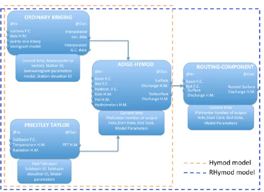
Finally, the runoff production is then propagated in the channel network. In this paper, a new runoff propagation component presented. To investigate the role and possibly the importance of the channel routing component a testing is performed. Two river basins are used for test and modeled in a three different delineations by using one (DL1), three (DL3) and twenty (DL20) HRU's. Two modeling solutions are setup: Hymod and RHymod Illus-trated in fig. (1).
The modeling solution RHymod includes: Pristley-Taylor component for the evapo-transpiration estimate, ordinary kriging algorithm for the rainfall spatialization, hymod model for the runoff production of the hillslope and finally the new channel routing com-ponent presented in the next section. The modeling solution Hymod differs from the model solution RHymod just because the channel routing component is turned off and the dis-charge for each HRU is simply summed going downstream. LUCA (Hay et al. (2006)) al-gorithm was selected for calibrating component for both the modeling solutions. The
ob-jective function is the Kling-Gupta efficiency (KGE) function presented in Gupta et al., (2009).
Figure 1. Modelling solutions: Hymod (in red dashed line) and RHymod (in blue dashed line).
3.1. The flow routing component.
As presented in Formetta et al. (2011) the flow generated for each hillslope is kinemat-ically propagated downstream in the channel network by integrating, in each channel link, a non-linear variant of the Saint Venant equation (e.g. Bras and Rodriguez-Iturbe (1994)).
For each link, the continuity equation is in fact:
dSi(t)
dt = Qgen(t) +
∑
tribQtrib(t) − Qi(t) # $ % & ' ( i = 1, 2,..., H (1)where Si(t ) is storage in the i-th link at time t, H is the total number of network links,
Qi(t ) [L3T-1] is the output discharge from i-th link, Qtrib(t) [L3T-1] is the flow of upstream
links, and Qgen(t) [L3T-1] is the discharge generated at the hillslope of the link in question.
Differently from Formetta et al. (2011) the routing component is modified taking into account the novel approach proposed in Mandapaka et al. (2009). Considering a generic cross section, the relation between the storage and the output discharge from a generic i-th link is:
Si(t) =
Qi(t)⋅ li vi(t)
in which li [L] and vi [LT-1] indicate, respectively, the length and the velocity in the
channel i-th. The velocity is estimated as presented in Mantilla (2001):
vi(t) = vr⋅ Qi(t) QR " # $ % & ' λ1 ⋅ Ai AR " # $ % & ' λ2 (3)
where Ai [L2] is the upstream area of the link, vr [LT-1], Qr [L3T-1] and Ar [L2], are
refer-ence velocity, discharge and area,
λ
1 and λ2 are the scaling exponents of velocity fordis-charge and upstream area, respectively.
Replacing the velocity in eq. 2 as proposed in eq. 3 gives:
Si(t) = Qi(t)⋅ li vr⋅ Qi(t) λ1⋅ A i λ2 (4)
where Qr and Ar are taken to be 1 [L3 T-1] and 1 [L2] respectively.
Deriving in time eq. 4, the left hand side of eq. 1 becomes:
dSi(t) dt = li⋅ (1−λ1) vr⋅ Qi(t) λ1⋅ A i λ2 ⋅ dQi(t) dt (5)
Finally, replacing eq. 5 in eq. 1, the continuity equation for the i-th link the ordinary becomes a non linear ordinary differential equation:
dQi(t)
dt = K Q
(
i(t))
⋅ Qgen(t) +∑
tribQtrib(t)− Qi(t) $ % & ' ( ) (6) where: K Q(
i(t))
= vr⋅ Qi(t) λ1⋅ A i λ2 li⋅ (1−λ1) (7)Eq. 6 has to be solved for each link i, i=1,2,..., H of the channel network.
Using the Pfafstetter scheme as described Formetta et al. (2011) the network from up-stream to downup-stream. Because of this reason the resolution of the set of routing equations starts from the upstream hillslopes (where the term Qtrib(t)
trib
∑
is null) and goes downstream(where the Qtrib(t) trib
∑
becomes a known term) according to the numbering rules. The procedure provides both the outgoing discharge and the mean velocity for each link i.4. Application
Different components of the framework JGrass-NewAge are applied in a cascading manner according to the methodology presented in Formetta et al. (2011). In sequence they are: the geomorphological analysis tools to extract the HRU, the river network and the ge-omorphological features used in the other components; the meteorological interpolator components for the spatialization of the meteorological variables (air temperature and rain-fall); potential evapotranspiration component; the runoff production and eventually the
routing component to compute discharge; the automatic calibration component to estimate the best set of model parameters; validation package component to compute some good-ness of fit indexes and to measure quantitatively the performance of the model.
For each delineation (DL1, DL3 and DL20) Hymod and RHymod modeling solutions were applied. One year calibration is performed by using the LUCA algorithm by optimiz-ing the KGE Gupta et al. (2009) objective function. Finally the simulation results are pre-sented both in a qualitative point of view by comparing measured and simulated hydro-graph and by a quantitative point of view, by computing two indices of goodness of fit: the index of agreement, IOA, Willmott et al. (1985) and the percentage model bias (PBIAS).
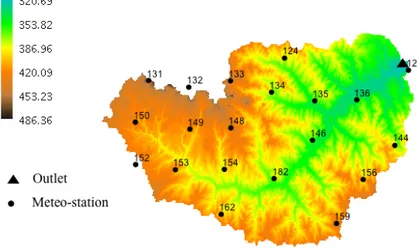
The test is performed on two different river basin: Fort Cobb and Little Washita. The Little Washita river basin (611 Km2 ), (Fig.2) is located in southwestern Oklahoma, be-tween Chickasha and Lawton.
Figure 2. The Little Washita river basin, Oklahoma (U.S.A.).
The climate of the basin can be characterized as sub-humid with a long-term, spatial average, annual precipitation of 760 millimeters and a temperature of 16 degrees Celsius. Winters are typically short and dry but are usually very cold for a few weeks. Summers are typically long, hot, and relatively dry.
The elevation of the basin ranges between about 300 meters and about 500 meters a.s.l. The bedrock exposed in the watershed consists of Permian age sedimentary rocks and soil textures range from fine sand to silty loam.
The meteorological stations used in this study are plotted in black dots in
fig. (2) and the hydrometer where the calibration is performed is depicted with a black tri-angle.
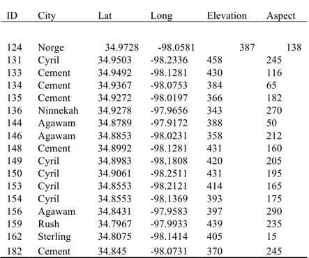
Table 1 reports the main information (coordinates and elevations) of the twenty mete-orological stations (whose data are available at http://ars.mesonet.org/). Five-minute meas-urements of rainfall (P), air temperature (T), and incoming solar radiation (R) were aggre-gated to hourly time steps and used as input of the modeling system. The stream gauge measures discharge at 15-minute resolution. The values were aggregated to hourly time step and used in the automatic calibration procedure.
Table 1. List of the meteorological stations used in the simulations performed
on Little Washita river basin.
ID City Lat Long Elevation Aspect
124 Norge 34.9728 -98.0581 387 138 131 Cyril 34.9503 -98.2336 458 245 133 Cement 34.9492 -98.1281 430 116 134 Cement 34.9367 -98.0753 384 65 135 Cement 34.9272 -98.0197 366 182 136 Ninnekah 34.9278 -97.9656 343 270 144 Agawam 34.8789 -97.9172 388 50 146 Agawam 34.8853 -98.0231 358 212 148 Cement 34.8992 -98.1281 431 160 149 Cyril 34.8983 -98.1808 420 205 150 Cyril 34.9061 -98.2511 431 195 153 Cyril 34.8553 -98.2121 414 165 154 Cyril 34.8553 -98.1369 393 175 156 Agawam 34.8431 -97.9583 397 290 159 Rush 34.7967 -97.9933 439 235 162 Sterling 34.8075 -98.1414 405 15 182 Cement 34.845 -98.0731 370 245
The Fort Cobb Watershed, fig.(3), is located in the Central Great Plains Ecoregion in south-western Oklahoma in Caddo. It is 813 square kilometres in size. Its elevation ranges between 383 meters and 565 meters a.s.l. Land use in the watershed includes agricultural fields, cattle operations, rural communities, and one hog feeding operation. Most soils in the watershed are highly erodible, sandy clays and loams underlain primarily by Permian sandstone, siltstone, and claystone.
The climate of the basin can be characterized as moist with a spatially average, annual precipitation of 816 millimeters and a temperature of 16 degrees Celsius. The JGrass-NewAGE modelling solution is applied for the Fort Cobb river basin at the Eakly outlet, before the river enters the reservoir.
Five minutes meteorological measurements of rainfall, air temperature and incoming solar radiation are available at http://ars.mesonet.org/ for the watershed. The data was ag-gregated to hourly time steps and used as input of the modelling system. Seven meteoro-logical stations were used in this study. Table 2 contains their main features.
Table 2. List of the meteorological stations used in the simulations performed on
Fort Cobb river basin.
ID City Lat Long Elevation Aspect
101 Hydro 35.4551 -98.6064 504 120 104 Colony 35.3923 -98.6233 484 35 105 Colony 35.4072 -98.571 493 300 106 Eakly 35.3915 -98.5138 472 295 108 Eakly 35.3611 -98.5712 492 40 109 Eakly 35.3123 -98.5675 466 90 110 Eakly 35.3303 -98.5202 430 115 113 Colony 35.291 -98.6357 465 155 182 Cement 34.845 -98.0731 370 245
The simulation period covered the two years two years: 2006-2007 in the case Fort Cobb and 2002-2003 in the case of Little Washita river basin; one year was used for cali-bration and one year for verification. The simulations time step was hourly.
5. Results
The Fort Cobb and the Little Washita river basin results are presented in table 3 and 4 respectively. Each row contains: i) the delineation type (DL1, DL3 and DL20); ii) the model solution (Hymod and RHymod); iii) the optimized objective function (KGE) value and the goodness of fit indices (IOA and PBIAS) for all the simulation period.
Table 3. Fort Cobb simulation results for different delineations and for
different model configurations
Delineation Modelling solution KGE IOA PBIAS
DL1 Hymod 0.53 0.79 24.4 DL1 RHymod 0.7 0.83 9.20 DL3 Hymod 0.65 0.81 13.01 DL3 RHymod 0.81 0.89 3.90 DL20 Hymod 0.63 0.8 18.4 DL20 RHymod 0.65 0.83 17.20
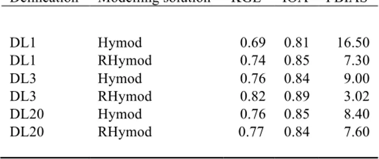
Table 4. Little Washita simulation results for different delineations and for
different model configurations
Delineation Modelling solution KGE IOA PBIAS
DL1 Hymod 0.69 0.81 16.50 DL1 RHymod 0.74 0.85 7.30 DL3 Hymod 0.76 0.84 9.00 DL3 RHymod 0.82 0.89 3.02 DL20 Hymod 0.76 0.85 8.40 DL20 RHymod 0.77 0.84 7.60
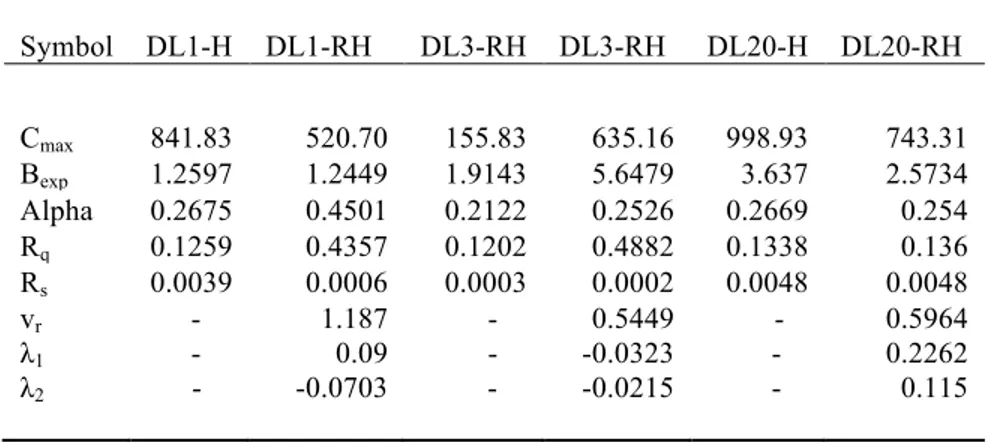
Tables 5 and 6 present the optimum values of the model parameters for both the model configurations (Hymod and RHymod) and for all the delineations (DL1, DL3 and DL20), respectively for Fort Cobb and Little Washita river basin.
From the quantitive analysis of the results it can be concluded that both modeling solu-tions, Hymod and RHymod, are able to simulate in a reliable way the discharge. Based on the goodness of fit indices, the total volume is actually better simulated using RHymod than Hymod model. In fact in the RHymod case the PBIAS shows lower values both for the Fort Cobb and for the Little Washita river basin. Moreover, the RHymod model is able to simulate both the peak values and the peak time, as is confirmed by better KGE and IOA values than Hymod in both the study cases.
Table 5. Fort Cobb river basin: parameter sets used in the simulations for RHymod (RH)
and Hymod (H) model for different delineations (DL1, DL3 and DL3
Symbol DL1-H DL1-RH DL3-RH DL3-RH DL20-H DL20-RH Cmax 906.05 403.80 141.3387 813.29 696.25 595.02 Bexp 1.7392 0.7204 2.1321 1.2697 1.1917 2.207 Alpha 0.2193 0.2487 0.1294 0.23 0.3616 0.3619 Rq 0.2261 0.3587 0.2088 0.2099 0.2288 0.2207 Rs 0.0008 0.0007 0.0001 0.0009 0.0012 0.0011 vr - 0.3132 - 0.6594 - 0.5806 λ1 - 0.7978 - -0.3915 - -0.5298 λ2 - 0.0750 - 0.842 - 0.3420
Table 6. Little Washita river basin: parameter sets used in the simulations for RHymod
(RH) and Hymod (H) model for different delineations (DL1, DL3 and DL3
Symbol DL1-H DL1-RH DL3-RH DL3-RH DL20-H DL20-RH Cmax 841.83 520.70 155.83 635.16 998.93 743.31 Bexp 1.2597 1.2449 1.9143 5.6479 3.637 2.5734 Alpha 0.2675 0.4501 0.2122 0.2526 0.2669 0.254 Rq 0.1259 0.4357 0.1202 0.4882 0.1338 0.136 Rs 0.0039 0.0006 0.0003 0.0002 0.0048 0.0048 vr - 1.187 - 0.5449 - 0.5964 λ1 - 0.09 - -0.0323 - 0.2262 λ2 - -0.0703 - -0.0215 - 0.115
On the other hand, the RHymod model has three more parameters than Hymod. It brings to increase the calibration convergence time and the optimal parameter spotting with respect to Hymod model that also provided acceptable results.
For both the river basins, the RHymod model, where the channel routing is explicit, provides better performances in the delineation DL3. The models' performances decrease in the case of delineation DL1. Even if RHymod outperformed Hymod model, this could be due to neglecting the rainfall spatial variability: a spatially uniform rainfall is applied in this case. In the case of the DL20 delineation, the use of RHymod and the explicit routing model did not provide any model performance improvement. This happened in both the river basins. This result confirms the findings of in D'Odorico and Rigon (2003) and Botter and Rinaldo (2003) where it is evidently shown that the hillslope (and not the channel) contribute with the largest part of the residence time. In the DL20 delineation HRU's size is the smallest. Moreover, at this scale, for both the basins up to 15-25 km2 , non linearity
in the process of runoff production could not be simulated well by a model based on linear reservoir (such as Boyle (2001))
Both models, slightly underestimated the highest peak flood values. This could be due to the fact that non-specific calibrations were performed for these events and to the implicit assumptions made in the classical formulation of Hymod Moore (1985) where residence time in the hillslopes does not depend on the soil moisture conditions. This is not in total agreement with what it is known of the hydrological problem and a possible solution could be the use of non-linear runoff generation models instead the linear model presented in this study.
6. Conclusions
The JGrass-NewAge system provides not only a new hydrological tool but a system in which any model can be built in components that can be independently modified or
changed. In this paper a verification of single parts of a modeling chain, keeping the others fixed, is performed. A new channel routing component is presented. Hymod and RHymod
hydrological models were set up: in Hymod, no routing component is used, and in RHymod, the new routing component is used. The two different modeling solutions are tested on Little Washita and Fort Cobb river basins and discharge simulations are per-formed. The basin delineation is also varied in order to understand the effect of the HRUs size.
Results show that the RHymod improved, even though not dramatically, the model re-sults in terms of discharge simulation. The model with the routing component performed best in the case of middle size HRUs (DL3). In the case of small size HRUs (DL20) there are no significant differences between the two modeling solutions.
The paper finally shows the possibility of a component by component and interopera-bility comparison on the same framework. For example the JGrass- NewAge system could be compared with others models, such as PRSM (Leavesley et al. (1983)) or J2000 (Krause (2001)) that embraced the OMS3 framework.
References
Antevs, E., 1954: Climate of New Mexico during the last glacio-pluvial. J. Geology, 62, 182-191.
Bailey, R. W., 1935: Epicycles of erosion in the valleys of the Colorado Plateau province. J. Geology, 43, 337-355.
Balling, R. C., and S. G. Wells, 1990: Historical rainfall patterns and arroyo activity within the Zuni River drainage basin, New Mexico. Ann. Assoc. Amer. Geog., 80(4), 603-617.
Allen, R., Pereira, L., Raes, D., Smith, M., et al.: Crop evapotranspiration- Guidelines for computing crop water requirements-FAO Irrigation and drainage paper 56, FAO, Rome, 300, 6541, 1998.
Bird, R. and Hulstrom, R.: Simplified clear sky model for direct and diffuse insolation on horizontal surfaces, Tech. rep., Solar Energy Research Inst., Golden, CO (USA), 1981.
Botter, G. and Rinaldo, A.: Scale effect on geomorphologic and kinematic dispersion, Water resources re-search, 39, 1286, 2003.
Boyle, D. P.: Multicriteria calibration of hydrological model, Ph.D. dissertation, Dep. of Hydrol. and Water Resour., Univ. of Ariz., Tucson, 2001.
Bras, R. and Rodriguez-Iturbe, I.: Random functions and hydrology, Dover Pubns, 1994.
Brutsaert, W.: Evaporation into the atmosphere: Theory, history, and applications, vol. 1, Springer, 1982. Brutsaert, W.: Hydrology: an introduction, Cambridge Univ Pr, 2005.
Corripio, J.: Modelling the energy balance of high altitude glacierised basins in the Central Andes., PhD dis-sertation, University of Edinburgh; 2002, 2002.
Cressie, N.: Statistics for spatial data, Terra Nova, 4, 613{617, 1992.
David, O., Ascough, J., Leavesley, G., and Ahuja, L.: Rethinking modeling framework design: object model-ing system 3.0, in: Environmental Modellmodel-ing International Conference Proceedmodel-ings, pp. 5-8, 2010. D'Odorico, P. and Rigon, R.: Hillslope and channel contributions to the hydrologic response, Water resources
research, 39, 1113, 2003.
Duffy, C. J.: A Two-State Integral-Balance Model for Soil Moisture and Groundwater Dynamics in Complex Terrain, Water Resour. Res., 32, 2421{2434, URL http://dx.doi.org/10.1029/96WR01049 , 1996. Eberhart, R. and Shi, Y.: Particle swarm optimization: developments, applications and resources, in:
Proceed-ings of the 2001 congress on evolutionary computation, vol. 1, pp. 81-86, Piscataway, NJ, USA: IEEE, 2001.
Erbs, D., Klein, S., and Due, J.: Estimation of the diffuse radiation fraction for hourly, daily and monthly-average global radiation, Solar Energy, 28, 293-302, 1982.
Formetta, G., Mantilla, R., Franceschi, S., Antonello, A., and Rigon, R.: The JGrass-NewAge system for forecasting and managing the hydrological budgets at the basin scale: models of flow generation and propagation/routing, Geoscientific Model Development, 4, 943-955, doi:10.5194/gmd-4-943-2011, URL http://www.geosci-model-dev.net/4/943/2011/ , 2011.11
Garen, D. and Marks, D.: Spatially distributed energy balance snowmelt modelling in a mountainous river basin: estimation of meteorological inputs and verification of model results, Journal of Hydrology, 315, 126-153, 2005.
Garen, D., Johnson, G., and Hanson, C.: Mean areal precipitation for daily hydrologic modeling in moun-tainous regions1, JAWRA Journal of the American Water Resources Association, 30, 481-491, 1994. Goovaerts, P.: Geostatistics for natural resources evaluation, Oxford University Press, USA, 1997.
Gupta, H., Kling, H., Yilmaz, K., and Martinez, G.: Decomposition of the mean squared error and NSE per-formance criteria: Implications for improving hydrological modelling, Journal of Hydrology, 377, 80-91, 2009.
Hay, L., Leavesley, G., Clark, M., Markstrom, S., Viger, R., and Umemoto, M.: Step wise, multiple objective calibration of a hydrologic model for a snowmelt dominated basin1, JAWRA Journal of the American Water Resources Association, 42, 877-890, 2006.
Helbig, N., Lowe, H., Mayer, B., and Lehning, M.: Explicit validation of a surface shortwave radiation bal-ance model over snow-covered complex terrain, Journal of Geophysical Research Atmospheres, 115, D18 113, 2010.
Iqbal, M.: An introduction to solar radiation, 1983.
Kennedy, J. and Eberhart, R.: Particle swarm optimization, in: Neural Networks, 1995. Proceedings., IEEE International Conference on, vol. 4, pp. 1942-1948, IEEE, 1995.
Krause, P.: Das hydrologische Modellsystem J2000: Beschreibung und Anwendung in grofen Flufegebieten, Forschungszentrum, Zentralbibliothek, 2001.
Leavesley, G., Lichty, R., Troutman, B., and Saindon, L.: Precipitation-runoff modeling system: User's man-ual, Available from Books and Open File Report Section, USGS Box 25425, Denver, Co 80225. USGS Water Resources Investigations Report 83-4238, 1983. 207 p, 54 _g, 15 tab, 51 ref, 8 attach., 1983. Lloyd, C.: Assessing the effect of integrating elevation data into the estimation of monthly precipitation in
Great Britain, Journal of Hydrology, 308, 128-150, 2005.
Mandapaka, P., Krajewski, W., Mantilla, R., and Gupta, V.: Dissecting the effect of rainfall variability on the statistical structure of peak flows, Advances in Water Resources, 32, 1508-1525, 2009.
Mantilla, R.: Physical basis of statistical self-similarity in peak flows on random self-similar networks, PhD dissertation, University of Colorado, Boulder; 2007, 2001.
Mantilla, R. and Gupta, V.: A GIS numerical framework to study the process basis of scaling statistics in riv-er networks, IEEE Geoscience and Remote Sensing Lettriv-ers, 2, 404{408, 2005.12
Monteith, J. et al.: Evaporation and environment, in: Symp. Soc. Exp. Biol, vol. 19, pp. 205{234, 1965. Moore, R.: The probability-distributed principle and runoff production at point and basin scales, Hydrol. Sci.
J., 30, 165, 1985.
Orgill, J. and Hollands, K.: Correlation equation for hourly diffuse radiation on a horizontal surface, Solar energy, 19, 357{359, 1977.
Penman, H.: Natural evaporation from open water, bare soil and grass, Proceedings of the Royal Society of London. Series A. Mathematical and Physical Sciences, 193, 120{145, 1948.
Priestley, C.: Turbulent transfer in the lower atmosphere, University of Chicago Press Chicago, Ill., 1959. Priestley, C. and Taylor, R.: On the assessment of surface heat flux and evaporation using large-scale
param-eters, Monthly weather review, 100, 81-92,1972.
Reindl, D., Beckman, W., and Du_e, J.: Di_use fraction correlations, Solar Energy, 45, 1-7, 1990. Slatyer, R. and McIlroy, I.: Practical Microclimatology., Practical Microclimatology., 1961. Vrugt, J., Ter Braak, C., Diks, C., Higdon, D., Robinson, B., and Hyman, J.:
Accelerating Markov chain Monte Carlo simulation by di_erential evolution with self-adaptive random-ized subspace sampling, International Journal of Nonlinear Sciences and Numerical Simulation, 10, 273-290, 2009.
Willmott, C., Ackleson, S., Davis, R., Feddema, J., Klink, K., Legates, D., ODonnell, J., and Rowe, C.: Sta-tistics for the evaluation and comparison of models, Journal of Geophysical Research, 90, 8995{9005, 1985.13