Hyetograph Simulation of High-Intense Rainfall Events
Franz Konecny
1Working Group Stochastic Hydrology, BOKU - University of Natural Resources and Applied Life Sciences, Vienna.
Peter Strauss
Institute for Land and Water Management, Petzenkirchen, Austria
Abstract. The simulation of storm hyetographs is an important issue for various applications in hydrology and soil sciences. In this study we present a modification of the simple scaling model of Koutsoyiannis and Foufoula-Georgiou (1993), which assume a piecewise linear relationship be-tween the logarithmic duration and logarithmic expected depth of an event. The expectation of the rainfall depth is estimated by local regression smoothing.
.
1. Introduction
Hyetographs (rainfall-intensity curves) picture the time distribution of point rainfall and are important for hydrologic and hydraulic design issues. In the study of soil erosion, spe-cifically on movement of soil particles by raindrop impact, kinetic energy is a commonly suggested indicator of the raindrop's ability to detach soil particles from the soil mass. The kinetic energy of raindrops can be estimated from rainfall intensity.
Since only rainfall with sufficient intensity is effective, we focus on high-intense rain-fall events. From historical rainrain-fall records, we
i. separate events from rainfall time series (6-hours-criterion) ii. use only events with total rain depth 15mm
iii. use only events with maximum intensity 10mm/hr
2. Summary of the Scaling Model of Storm Hydrograph
The scaling model of storm hydrograph (Koutsoyiannis and Foufoula-Geor-giou, 1993) is a stochastic model that describe the time distribution of rainfall intensity and incremental rainfall within a storm event, taking advantage of scaling properties revealed in rainfall data.
1 Working Group Stochastic Hydrology BOKU –University of Natural Resources and Applied Life Sciences, Vienna Muthgasse 18
A-1190 Vienna Austria
The main hypothesis of the model is that the process of instantaneous rainfall intensi-ties within storms is a self-similar (simple scaling ) process with a scaling exponent H. If
D denotes the duration of the storm and the rainfall intensity at time , then
(1)
where the symbol denotes equality in distribution. A secondary hypothesis is the weak stationarity within the same storm event or within storm events of the same duration. On the basis of these hypotheses, the moments of the rainfall intensity at any time t within a storm of any duration D can be deduced. The expectation value is
(2) and the product moment
(3)
where is a time lag, and is a function to be specified. In this pa-per we specify this function as .
(4)
where and are parameters ( , ).
The total storm depth over duration D,
(5) has the mean
(6) and the variance
(7) where is the variance of the depth of a storm with duration D = 1.
Moving from continuous time to discrete time we use the incremental storm depth at the interval of length :
i=1,2,…,k (8)
where is assumed to be an integer. The expectation of is (9) its variance is
(10)
where .The covariance between two incremental depths within the same storm is given by
(11)
where . The derivations of the above
equa-tions are given by Koutsoyiannis and Foufoula-Georgiou (1993) .
The scaling model, in its simplest form, has four parameters: the scaling exponent H, the expectation parameter , the variance parameter and the covariance decay parameter
. Taking the logarithms in (6) we get
. (12)
By local regression smoothing we can estimate in dependency of D. Thus H and are directly estimated by least squares from (12), and from (7). The parameter is es-timated directly from the identity
(13) which was derived from (9) and (11) in Koutsoyiannis and Pachakis (1996).
3. The Modified Scaling model
In Koutsoyiannis and Foufoula-Georgiou (1993) a global validity of the linear relation-ship of and is taken for granted. But scatterplots like Fig. 1 indicate a more or less significant deviation of the linear relationship.
In surprisingly many cases a single breakpoint is present and the scaling property is (ap-proximatively) valid, above and below this breakpoint with different scaling expo-nents. Typically is located in the range of 19 to 22 hours. Setting
and we get from (12)
(14) .
A piecewise linear regression line has to satisfy the constraint The pa-rameters in (14) are estimated by least squares method subject to the constraint The procedures for least square estimation under constraints can be found in most textbooks on regression analysis, e.g. Draper and Smith (1998).
The modified scaling model has seven parameters: the expectation parameters and , the variance parameter and , the scaling exponents and
and the covariance decay parameter . Since the r.h.s. of (13) does not depend on D is a global parameter.
4. Case Studies
As test cases for the modified scaling model, data sets from three rain gauges were used: a rain gauche at St. Pölten, Lower Austria, one at Steyr, Upper Austria, and a rain gauge at Baden, Lower Austria. The available time resolution is 5 min and the depth resolution is 0.01 mm.
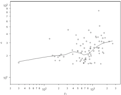
Using the criterion stated in the introduction, a data set of 164 events were extracted. Fig. 2 shows a scatterplot where against was plotted. The solid line is a re-gression curve obtained local rere-gression smoothing. As a smoothing tool we used the rou-tine loess.smooth of S-Plus (2001). The curve shown in Fig. 2 exhibits no distinct break-point. So the original scaling model with a global scaling exponent can be used. The local regression function estimates for a given duration time D the value of E[Z]. This estima-tion method seems to us more efficient than the rough grouping approach used in Koutsoy-iannis and Foufoula-Georgiou (1993). The estimates of E[Z] were inserted in (12) to per-form the parameter estimation procedures described in section 2.
For the data set St. Pölten the following estimates were obtained:
(15)
Figure 3. Scatterplot and local regression curve
Fig. 3 depicts the scatterplot of the data set Steyr consisting of 220 storm ev-ents. The re-gression curve exhibits a bend and a breakpoint near 20.8 h. The location of the breakpoint was estimated such that squared deviation of the piece-wise linear model given by (14) from the regression curve is minimal (see Fig. 5). In the range below the breakpoint
the following estimates were obtained:
, (16)
in the range above the breakpoint
Figure 4. Scatterplot and local regression curve
Fig. 4 depicts the scatterplot of the data set Baden consisting of 220 storm events. A breakpoint was found near 23.2 h. Again a piece-wise linear model was fitted with = 7.24. Below the breakpoint we obtained the estimates
, (18)
above we obtained
. (19)
Fig. 5 and 6 shows the local regression curves and the corresponding piece-wise linear models for the data sets Steyr and Baden, respectively.
5. Simulation of storm hyetographs
The scaling model can be used for simulating storm hyetographs at an incremental basis for any time step . In our simulation studies we used the disaggregation procedure where a given total storm depth Z with a duration D is disaggregated into incremental depths. We have to generate a random vector X , where is assumed to be an integer. The covariance structure of X is given by the scaling model, cf. formula (11). Moreover we have to specify the marginal distribution. For rain-fall depths the Gamma distribution is the first choice. Let Z = be a k-vector of two-parameter Gamma distributed random variables with
.
Figure 5. Local regression curve and piecewise-linear model
identity covariance matrix. Sim (1993) proposed a procedure to generate X by a linear transformation
X = B Z. (20)
B is a lower triangular matrix of Beta distributed random variables. Some details of Sim’s
method are given in the appendix. Different from the sequential process proposed by Koutsoyiannis and Foufoula-Georgiou (1993), Sim’s procedure results always non-negative exactly Gamma distributed output.
Making use of the scale invariance the total storm is disaggregated by the following proc-ess:
i. Apply Sim’s procedure to obtain an initial sequence . ii. Determinate a normalize sequence
. (21)
iii. Calculate the final sequence .
A disadvantage of Sim’s procedure is that the given covariance matrix must
have positive entries, that is all the components of the random vector X must be posi-tively correlated.
6. Conclusions
A modification of the simple scaling model has been presented, with different
scaling exponents for small and large storm durations. The expected storm depth, as a function of storm duration, was estimated by local regression smoothing. A piecewise lin-ear model was fitted by least squares estimation. So the scaling model can be used even in the case of nonlinear relationship of and log D. The presence of a single break-point was observed in many data sets of storm events.
Koutsoyiannis and Mamassis (2001) compared the simple scaling model with the rec-tangular pulse model of Rodriguez-Iturbe et al. (1987) applied to a single storm tograph. They found that the scaling model reproduces the structure of historical hye-tograph better than the rectangular pulse model. Recently Cowpertwait et al. (2007) pro-posed a refined rectangular pulse model with an appropriate fine-scale structure. A com-parison of the modified scaling model with a refined rectangular pulse model will be the subject of a further study.
Appendix
In this appendix we give a short description of Sim’s generation process, specialized to our simulation problem. Let Z = be a k-dim-ensional random vector with identity covariance matrix and Gamma( ) marginal distributions. Let
be independent Beta( )
random variables which are independent of , and . The required gamma
ran-dom vector X which has given Gamma( ) marginal distributions
and a given covariance matrix , where , can be obtained via the trans-formation (20), with . The random variables have Gamma( ) marginal distributions. The aim is to determine the coefficients and parameters given , and via the recursive formula
(22) and . (23)
Note we have to ensure, that This conditions are required by the construction of (20). It means that this simulation procedure will stop if any of these pa-rameters goes beyond these intervals.
References
Cowpertwait, P., V. Isham and C. Onof, 2007: Point process models of rainfall: Developments for fine-scale structure. Proc. R. Soc. A 463, 2569-2587. Draper, N. R. and H. Smith, 1998: Applied Regression Analysis, 3rd Edition.
J. Wiley, New York.
Koutsoyannis, D and Foufoula-Georgiou, E. 1993: A scaling model of storm hyetograph. Water
Resour. Res.. , 29(7), 2345-22361.
Koutsoyannis,D. and D. Pachakis, 1996: Deterministic chaos versus stochasticity in
analysis and modeling of point rainfall series. J. Geophys. Res., 101 (D21), 26441-26451. Koutsoyannis,D. and N. Mamassis, 2001: On the representation of hyetograph
characteristics by stochastic rainfall models. J. Hydrol. 251, 65-87. Rodriguez-Iturbe, I., D.R. Cox and V. Isham, 1987: Some models for rainfall based on stochastic point processes. Proc. R. Soc. Lond., A 417, 283-298.
Sim, C. H., 1993: Generation of Poisson and gamma random vectors with given marginals and co-variance matrix. J. Statis. Comput. Simul., 47, 1-10