Analysis of Colorado precipitation

ANALYSIS OF

COLORADO PRECIPITATION by

Marie Kuo and Stephen K. Cox

June 1975

Colorado State University -Fort Collins,Colorado

Completion Report Series No. 63

ANALYSIS OF COLORADO PRECIPITATION Completion Report

OWRR Project No. A-01B-COLO

by

Marie Kuo and Stephen K. Cox

Department of Atmospheric Science Colorado State University

submitted to

Office of Water Resources Research U.S. Department of the Interior

Washington, D. C. 20240

June 1975

The work upon which this report is based was supported (in part) by funds provided by the United States Department of the Interior, Office of Water Resources Research, as authorized by the Water Resources Research Act of 1964, and pursuant to Grant Agreement No. 14-31-0001-A-018-COLO.

Colorado Water Resources Research Institute Colorado State University

Fort Collins, Colorado 80523 Norman A. Evans, Director

TABLE OF CONTENTS

1.

ANALYSIS OF PRECIPITATION TREND

. .

.

.

.

..

.

.. ..

.

.

.

. .

.

1.1 Trend Analysis 1

2. CORRELATION BETWEEN

STATIONS

. . . .

8 3. STORM INFORMATION • • • • • • • • • • • • • • • • • • .. • • • 9

3.1 Data Source . . . 12

3.2 Division of Colorado into Six Regions 12 4. STORM

ANALYSIS

. . . 20

4.1 Storm Characteristics

22

4.2 Seasonal Comparison . e • • • • • • • • • • • • • • 25 4.3 Event Analysis 27 5. APPLICATIONS • • • • . . • . • . . • . • . • . • • • • • • • 33 6. SUMMAR Y • D • • • • • • • • • • • • • • • • • • • • • • • • • 35 REF ERENCES • • • • • . . . . • 0 • • • • • • • • • • • • • • 36

Completion Report

ABSTRACT

'ANALYSIS OF COLORADO PRECIPITATION'

The objectives of the research proposal 'Anlaysis of Colorado

Precipitation' fall into two categories. Firstly, 56 years of precipitation history were used to determine if there are any significant trends in

regional and statewide precipitation in Colorado$ This portion of the research is complementary to the work of Sellers (1960) who used the 90 year running mean of annual precipitation for 18 stations of Arizona and western New Mexico.

Secondly, 20 years of Colorado hourly precipitation data

were

used to represent precipitation events, called 'storms't and the data were examined to find storm frequency, length and yield. The storms were divided into size categories and were used to determine the contribution of each size of precipitation event to the annual total. Data from the western part of the state has been studied extensively because it is part of the upper Colorado River Basin which supplies water to the arid southwestern United States. Marlatt and Riehl (1963) found that most of the precipitation is produced in a few days and the amount of precipitation is correlated with the fraction of area receiving precipitation. In a comparison paper by Riehl and Elsberry (1964), consecutive days with precipitation were grouped together to form stormSe The precipitation derived from medium size stonms of 0.3 to 1.2 inches were found to be most closely related to the annual precipitation in the basint and the size of storms roughly corresponds to the duration of the episode.

-1-1. ANALYSIS OF PRECIPITATION TREND

Colorado has an area of 104,247 square miles with approximately 300 weather stations distributed throughout the state. Sixty-one of these Colorado stations have precipitation records of fifty

years

or longer.

1.1 Trend Analysis

The 61 long-term stations used in this analysis are listed alphabetically in Table 1. The locations of the stations are shown in Figure 1.

A straight line was fitted through a time series of annual precipitation data from each station to detect any increasing or decreasing precipitation trend (Draper and Smith, 1966). The slope and correlation coefficient were calculated for each of the long-term stations. The results are shown in Table 1. The average slope of all the stations is -0.009 inches per year i.e., an average decrease of one inch every 120 years.

To see if the apparent decrease in precipitation is due to the natural variability of the annual precipitation or to a change in climatic regime, a correlation coefficient between the annual precipitation and time was calculated. The results are shown in Table 2.

A histogram of the correlation coefficient is plotted in Figure 2. The distribution ;s normal with an average correlation of 0.07 and 47 percent of the stations have correlations in the interval between -0.15 and 0.0. If this average correlation coefficient is assumed to be constant and none of the other parameters change, it would take app~oximately 800 years of data for a correlation of 0.07 to be significant at the 5 percent

I N I 102 Springfield

•

e Eads

,

I

----103

---_I

I

iSter'~ng \ I ---!-Leroye 1--F---, Fort I I M~rg~nI

I.

Yuma I I 104 ..

_----I Grover

•

105 106

,----,

_"

, \ 107

.--I

,

I

J

,-I

- __ J. __

Meeker e 108 ~----.. 109 37 Fort , , C o l l i n s ,I Steamboat \ Estes • f

·0

.Spicer (\ Pork Waterdale.Greeley I

Spnn~~___ \ . . •

k'

I I , _ _ - ,....r.ongmont • I \Longs

II

f I 'Peak .Boulder • ~- .Hawthorn;--I - , J _{I -- ---'--,} Fraser t-=-~ r - - - \. \ ,-- ... I Denver I I , " ( I d h ' I • " - - -

-l

--_,...-~--r ShOS~00e ' , .... a ~.'i Edgewater

Rifle • • I Dillon. FSpr.!.n~ ..l - _ _ _ _ _ I - - ,

-• Glen~ood \' too: ,Kassler

I

I

Springs I

I

I

I

---r-

---r--, I , ' t

FruifoGrand '.COlbra~ Leadvillee { C h e e s m a n e , l ,

I .

I

e "'I " ' I Monument • Limon

J to- .Palisade / - - I I Hartse (- - - 1 I , _

-39 ~ unc Ion ---~ , _ _ _ . I e - _0

,,/ Paonial C r e s t e d ' IrLake

f - " • t eButte --:, " I ~...-° eColorado'

I e Delta

I

~ I -LMorolne Springs

I

I~"'- - - - Pitk~n, r - - - - _ I I --I

- - _ J Montrose • . ( ) Canon

J---,

I

-•

I

Gunnison •_{---~-- \} e

I

I

\ ' - _ \ 1 I \ City I • I Ordway. _ _ '\ I , , - - - - Pueblo • J

I

Las I I_L ) _{, A·}

I

_ornar

- - - -

....

\--',---

\

I

---.-# I ",mas• • 38 -, Te'~t.;rde - I m .., Ames. _",,- r '"""" '","""- 't _ Rocky

' - - / ilverton : L Center ( - - .... '.... t Ford Ro "-' f 'I , / ""

J

ICO J I H- Of - - _ . . - - - , , _ _ - - - • L.!-_' erm, I r'\ I - -

I

Cascad~

I , '

/

e., I • I I , I

r

I

J

Durangor--- - -\.. - - - - _ / J - - " I , • I

I

\

Fort Lewis - I .... , , . 'e North I

I .Manassa e --_L_ __~g~c:c~

\

l. __

J_

La~e_T~~~d 41 40 COLORADO _o 10 20 I I I Statute Miles

-3-TABLE

1

SUMMARY OF LONG-TERM STATIONS

AND~

THEIR TRENDS

SIGNIFICANT

NAME

LENGTH OF

DATE OF

SLOPE

CORRELATION

LEVEL

RECORD

RECORD

in./yr.

COEFFICIENT

5% 10%

Arnes 57 1914-1970 .028 .09 Boulder 78 1893-1970 .016 .08 Burlington 80 1891-1970 -.025 -. 12 Canon City 74 1897-1970 .001 .01 Cascade 51 1907-1959 -.114 -.20 Cheesman 68 1903-1970 -.007 -.04 Cheyenne Wells 74 1897-1970 -.029 -. 13 Collbran 75 1892-1966 -.034 -.21 X Colorado Springs 79 1892-1970 .081 .10 Crested Butte 61 1910-1970 .054 .14 .-Delta 83 1888-1970 -.006 -.07 Denver City 99 1872-1970 -.016 -.12 Dillon 58 1913-1970 -.048 -.23 X Durango 76 1895-1970 -.013 -.05 Eads 54 1917-1970 .011 .04 Edgewater 53 1909-1961 -.033 -. 12 Estes Park 61 1910-1970 -.092 -.33 X X Fort Collins 84 1887-1970 -.000 -.00 Fort Lewis 59 1912-1970 -.009 -.03 Fort Morgan 82 1889-1970 -.023 -.16 Fraser 61 1910-1970 -.008 -.04 Fru ita 63 1908-1970 -.050 -.33 X· X Glenwood Springs 61 1910-1970 .008 .04 Grand Junction 79 1892-1970 -.002 -.02 Greeley 79 1888-1966 -.015 -.10 Grover 58 1912-1969 -.016 -.07 Gunnison 70 1901-1970 .023 . 19 Hartsel 57 1909-1965 -. 011 -.06 Hawthorne 61 1910-1970 -.026 -.10

-4-TABLE 1 - Continued

SIGNIFICANT

NAME LENGTH

OF

DATE OF

SLOPE

CORRELATION

LEVEL

RECORD RECORD in./yr.

COEFFICIENT

5% 10%

Hermit 61 1910-1970 -.065 -.27 X X Idaho Springs 66 1905-1970 .005 .03 Ignacio 57 1914-1970 -.072 -.29 X X Julesburg 59 1912-1970 -.024 -.09 Kassler 72 1899-1970 .019 .09 Lake Moraine 69 1895-1963 -.031 -. 12' Lalnar 82 1889-'1970 -.014 -.08 Las An;nlas 104 1867-1970 .011 .09 Leadville 63 1908-1970 -.055 -.' 23 X Leroy 82 1889-1970 .031 .18 L;nlon 63 1908-1970 .014 .06 Longmont 60 1911-1970 -.041 -.18 Longs Peak 53 1895-1943 .070 .21 Montrose 71 1900-1970 .003 .02 Monument 53 1911-1963 -.011 -.04 Ordway 50 1921-1970 -.003 -.01 Palisade 59 1912-1970 -.031 -.20 Paonia 71 1900-1970 -.013 -.08 Pitkin 61 1910-1970 .043 .20 Pueblo 84 1887-1970 -.007 -.05 Rico 61 1910-1970 .030 .09 Rifle 59 1912-1970 -.012 -.07 Rocky Ford 82 1889-1970 -.017 -. 11 Shoes hone 61 1910-1970 .085 .40 X X Silverton 64 1907-1970 -.095 -.31 X X Spicer 61 1910-1970 .067 .45 X X Springfield 56 1915-1970 -.039 -.14 Steamboat Springs 62 1909-1970 -.016 -.07 Sterling 61 1910-1970 -.007 -.04 Telluride 59 1912-1970 .011 .03 Waterdale 76 1895-1970 -.008 -.04 YUlna 80 1890-1970 .010 .05

-5-TABLE 2

SLOPE AND CORRELATION COEFFICIENT

OF AVERAGE ANNUAL PRECIPITATION

S r

NUMBER

SLOPE IN

CORRELATION

OF YEARS

DATE

INCHES/YEAR

COEFFICIENT OF DATA

19 Stations with no -.021 -. 14 58 1913-1970

estimated values

29 Stations with estimated -.016 -.10 56 1914-1969

values

21 Eastern slope stations -.016 -.08 55 1915-1969

14 Western slope stations -.011 -.06 57 1914-1970

7 Oil shale stations -.025 -.17 55 1912-1966

Whole state weighted by -.009 -.06 56 1910-1965

area contributed by 43 stations

.45

.35

.25

-.15

-.05

0

.05

.15

CORRELATION COEFFICIENT

-.25

o"

AA At .\ A~A/\~A·\ '-,,Ar·.~ ~\!\

"It

"f\""I\""r.J\M!vjAM!\.~.l\''\f'J'\t\Mt''\MMI\/\M/\MMMMMMN\I\MN\/\I\f\I'v\:YV\\/VW I fJVyvyvv",vvvvV~~J

-.35

10

9

8

(J)

7

z

0

r-

6

<t l-(f) \ t - 5 0

I

cr:

WlfNffMVv\\~

w

4

(I) ~

~

3

I

I 0'\ I

2

-7-not constant, thust both the slope and correlation are not constant. If

any real trend exists, the correlation .coefficient would become significant in a much shorter time period.

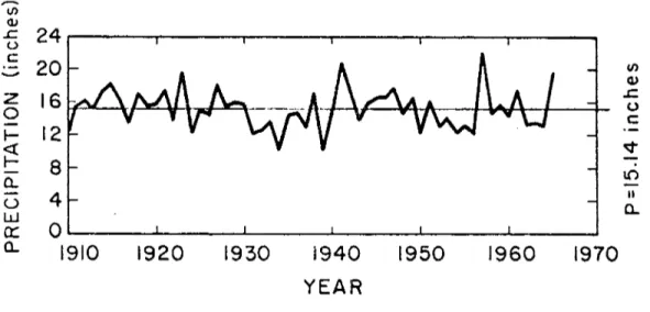
The annual area weighted precipitation of Colorado from 1910-1965 is shown in Figure 3. There are extended periods of relatively dry and wet years. The overall picturet however, does not show any noticeable

increase or decrease of precipitation.

,,-.-tf) Q) .c. ₂₄ u c 20 ..., VI cu z ₁₆ .s= 0 (J

-

c: I- 12 <! ~ i- _S

-

lO a..

-

₄

..

U Q. W

a::

0 a. _{1910 1920 1930 1940 1950 1960 1970}

YEAR

Figure 3. Area weighted precipitation of Colorado 1910-1965.

In conclusion, there was found no statistically significant trend in the statewide precipitation even though several individual stations do show long term trends.

-8-2.

CORRELATION BETWEEN STATIONS

It would be useful to find out if the precipitation measurements from a few stations are representative of the area concerned. Since precipitation in an area is always approximated by measurement at a location, a test of how well the data at a station approximates data from other stations in the same vicinity may give an indication of how well a station may represent an area.

Climatically, precipitation in Colorado is deposited by different mechanisms associated with the two seasons separated by transition periods.

In the winter, the precipitation is usually generated by storms of cyclonic scale of 500 to 1000 miles. Precipitation accompanying the storm generally occurs over a large area so that any analysis of correlation of precipi-tation between adjacent sprecipi-tations should yield high correlation coefficients. In the summer, the weather is brought about by small disturbances in the upper atmosphere of the same scale as the winter, but they are much weaker and do not have precipitating storm systems associated with them. Instead, the waves set up atmospheric conditions conducive to convective activity producing thunderstorms over the entire region. These thunderstorms have diameters oflO to 20 miles accounting for most of the summer precipitation. Since the activity occurs over a large area producing numerous thunderstorms in the region, correlation should exist, but because of the small

precipitating area, the correlation may not be as high as in the winter. To see how well the precipitation between adjacent stations agree, a correlation coefficient was calculated. The twenty-one long-term

-9-stations and their three surrounding -9-stations used are listed in Table 3. Correlation coefficients were computed between the precipitation of the long-term station with the average precipitation of three stations around it for twenty years. The monthly and annual correlation coefficients for each station are shown in Table 4. Referring to the monthly values, the poorest correlation occurs in July and August, and in October 50 percent of the stations have their best correlation. To compare the correlations obtained for the winter months (October - March) with those for th~ summer months (April - September), a mean correlation coefficient was calculated

by averaging the correlations for all stations for the appropriate season. The average summer correlation ;s 0.78 compared to 0.85 in the winter. SOt

as expected, the precipitation of adjacent stations correlates better in the winter than in the summer but the difference between them is small. Even though a large part of the summer precipitation is deposited by small scale thunderstorms, the correlation is still statistically significant at the 5 percent level. The annual precipitation is highly correlated between the stations and their surrounding stations. The coefficient is statisti-cally significant at the 1 percent level for each station. This suggests that on a year to year basis, a station may represent its surrounding area and that correlation exists. This result is as expected and is presented to support the contention that a station is representative of an area over a year in spite of the summer convective precipitation events.

3. STORM INFORMATION

In this section, values of hourly precipitation are manipulated to form natural precipitation periods. The hourly precipitation data supply statistics which describe precipitation variation in time: the mean annual rainfall and monthly distribution. These hourly precipitation data, however,

-10-TABLE 3

LIST OF STATIONS USED AND THEIR SURROUNDING STATIONS

NAME Boulder Canon City Delta Denver Durango Fort Collins Glenwood springs Grand Junction Gunn i son Las Anirnas Leroy Longmont Montrose Pitkin Pueblo Rocky Ford Silverton Springfield Stealnboat Sprin~s Telluride YUlua SURROUNDING STATIONS

Denver, Longmont, Allenspark Westcliff, Penrose~ Pueblo Montrose, Cedaredge, Palisade Denver AP, Boulder, Castle Rock

Mesa Verde, Silverton, Wagon Wheel Gap Greeley, Longmont, Nunn

Shoeshone, Eagle, Rifle Fruita, Palisade, Rifle Crested Butte, Wilcox Ranch,

Cochetopa Creek Lamar, Eads, Ordway

Sterling, Akron FAA, Yuma Greeley, Boulder, Allenspark Paonia, Delta, Norwood

Buena Vista, Gunnison, Crested Butte Fountain, Penrose, Ordway

Pueblo, Ordway, Las Animas

Telluride, Durango, Wagon Wheel Gap Granada, Kimt John Martin Dam

Spic(~r, Hayden, Yanlpa

Ouray, Silverton, Pleasant View Leroy, Akron FAA, Wray

TABLE 4

MU~THLyt SEA~orL~L MlD ANNUAL CORREL';TI'1~J Cf)EFFICIEr~T OF PP.fCIPITf\TIOr,·: 8F THE

LONG-TfRi-1 STATIONS WITH THE. AVERAGE PRECIPITATI0:~ OF THi{EE SURi{OUNDI~:G S:.l\lIONS.

NAt·~E J~\~. FE8. ~J'\R. P,~R. M/t", t JUNE JUL'" AUG. SEPT. OCT. l~OV. DEC.

s.

.,~. Ar::iUJ\L

- - - -Boulder .73 .78 .80 .96 .94 .€4 . ]0 .57 .93 .93 .64 .37 .82 .80 •g"L Canon C~ty .90 .UO .87 .94 .95 .73 .72 .73 .87 .95 .91' .74 .32 .86 .89 Del to .93 .C4 .92 .83 .89 .95 . 71 .82 .~~ .93 .84 .7i' .86 .87 .93 Def1ver •9'''\L _{.87 .86 .95 .94 .81} .9(: _.c9 .93 .97 .73 .90 .37 .38 .93 [)urango .JJera .92 .89 .86 .87 .72 .67 .55 .93 .87 .65 .94 .78 .87 .90 Fort Collins .84 .85 .95 .91 .89 .84 .62 .71 .94 .98 .85 .78 .82 .87 .89 -:

Glenwood Springs .76 .82 .8~ .e4 .86 .89 .84 .66 .93 .97 .46 .87 .84 .79 .87

Grand Junction .87 .81 .94 .,81 .87 .85 .78 .87 .93 .94 .80 .94 .85 .89 .93 Gunnison .93 .85 .81 .44 .8G .83 .76 .54 .78 .91 .ES .62 .70 .83 .75 las Ani~as .94 .97 .94 .96 .79 .84 . (1 .46 .75 .92 .84 .92 .73 .92 .77 I Leroy -.91 .83

..

9' .94 .94 .34 .47 .67 _.0",~~ _{.96 .93 .85} .79 .. 90 _.75 ~ ~ I Longmont .77 .65 .91 .92 .91 .80 .53 .42 .91 .94 .78 .69 .76 .79 .88 Montrose .57 t=~ .85 .78 .91 .83 .73 .62 .95 .67 .71 .43 .81 .68

.s:

aU..) Pitkin .88 .8i .86 .59 .90 .90 .70 .69 .95 .90 .76 .86 .79 .$.14 .66 Pueblo .S4 .68 .54 .37 .77 .68 .62 .3:; .84 .60 .92 .93 .65 .77 67 Rocky ford .92 .91 .90 .91 .83 .85 .3~ .54 .01 .97 .95 .91 .69 .93 .73 Si 1verton .83 .94 .90 .73 .89 .~a .73 .71 .94 , ' \ , \ _.87 .. 94 .81 .90 .88

.

~'--Springfield .90 .82 .64 .76 .93 .83 .56 .08 .69 .e3 .87 .82 .64 .81 .79

Steamboat Springs .84 .79 .e7 .81 .86 .90 .i9 .42 .96 .97 .83 .97 .79 .88 .90 Telluride .83 .94 .86 .84 .81 .87 .68 .72 .88 .9t .89 .86 .80 8{\ .83

• :I

Yuma .89 .83 .80 .94 .74 .91 .49 .76 .91 .95 .93 7? .79 .8~ .73

AVERAGE .78 .85 .84

-12-do not include information such as the number of storm occurrences in a year, their duration and the water yielded by each storm. The storm events were computed to give a better picture of how storm passage contributes to the water yield, and to see how precipitation varies in space. time and amount.

3.1 Data Source

Storm data were assembled from hourly precipitation ·data records over a twenty year period (1951-1970). From 1951 to 1967, precipitation was recorded to one hundredth of an inch. Beginning in 1968,

many

stations began using the Fisher-Porter gauge. This rain gauge punches a mark on paper tape whenever one tenth of an inch of precipitation is recorded. Thus, the resulting data is not the exact hourly precipitation, but rather,

indicates the amount of precipitation between the two time periods when precipitation had been recorded. Precipitation in increments less than 0.1 inches occurring during one day may not have been recorded until many

hours later, and therefore, may have been included in another storm. 3.2 Division of Colorado Into Six Regions

Colorado is a mountainous state whose elevation varies 10,000 feet within its boundaries. This wide range in elevation causes large

variations in the local climate and especially in orographic precipitation. It would be useful to group stations in the same geographic area together into a region so that the precipitation regime within the area would be more homogeneous. The topography of Colorado and its regional divisions are shown in Figure 4~ The Continental Divide runs in a north-south direction, approximately through the middle of the state. To the east, the land flattens to the high plains which makes up about 40 percent of

I

...

W I

•

GRANADA o 10 20 ECKLEY

•

ARAPAHOE-PAOLI

-JOES

•

EADS

•

Region 5 .AKRON Region 6

CHERAW JOHN MARTIN

•

DAM

•

_BRIGGSDALE GREELEY - NEW

-RAYMER Region Statute Miles I I I

Fig'lre 4. Topographic map of Colorado and the locations of regions and stations whose

-14-the area of -14-the state. To the west, the elevation decreases slightly and there are smaller mountain ranges extending in various directions. The state was divided into six regions to differentiate climatic differences due to topography. The number of stations in each region varies a great deal. The precipitation stations tend to be situated in population centers and are generally found near rivers or are located at the bottom of a

valley. Also shown in Figure 4 are the locations of the precipitation stations.

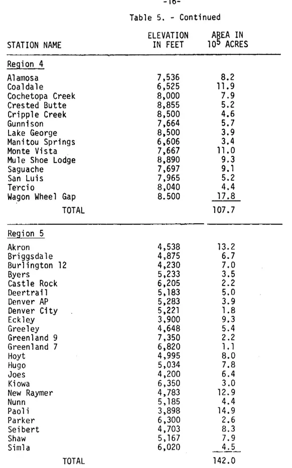
The stations in each region with their areas and elevations are listed in Table 5. The stations used have the longes~, most consistent hourly precipitation records. Although a few stations have had names changed or have been moved up to several miles, their precipitation data were used without any adjustment.

3.2.1 Precipitation Characteristics in the Six Regions of Colorado To illustrate how the precipitation of one region differs from another as an indication of the validity of the regional divisions, the average monthly precipitation of each region is shown in Figure 5. These average values were taken from the Monthly Normal Precipitation 1941-1970, and subdivided into the same six regions. Region 1 is the oil shale area which receives precipitation during both the winter and the summer months but it is dry throughout. Region 2, the southwest corner, also receives precipitation throughout the year, but has a maximum from July to October.

Region 3 ;s mainl.y Illounta1nous and receives more precipitation in the sumner

Inonths than in the winter Inonths. The annual precipitation of the stations in Region 3 are not as homogeneous as one would like; this region includes a few front-range stations which individually display a distribution

-15-TABLE 5

LIST OF STATIONS IN EACH REGION STI\TION NAM[

ELEVATION

IN FEET

AREA IN

105 ACRES 5,921 18. 1 6,285 15. 1 4,855 23. 1 7,030 12.5 6,242 14.5 5,400 11 .3 94.6 TOTAL Region 1

Artesia - Dinasaur National Monument Craig Grand Junction Great Divide Meeker Rifle R~.9jon 2 Cedaredge Durango Mesa Verde Ouray Pleasant View Silverton Telluride Wilcox Ranch TOTAL 6,175 6,550 7,070 7,740 6,860 9,322 8,756 5,960 11 •7 12.4 8.3 7.3 15.5 6.8 10.3 9.0 81.3 Region 3 Allenspark Aspen Boulder Clinlax Eagle FAA Elk Creek Evergreen Fort Collins Grand Lake

Hartsel - Antero Reservoir Hot Sulphur Springs

Longmont Morrison

Sugar Loaf Reservoir Woodland Park TOTAL 8.500 7,928 5,400 11,300 6,497 8,430 7,000 5,001 8,288 8,866 7,800 5, 145 6,000 10,000 7,760 5.8 5.8 2.8 6.7 14.5 4.7 2.7 8.2 12. 1 7.5 16.5 3.5 1.6

&.4

2.9 101. 7

-16-Table 5. - Continued ELEVATION _A~EA

IN

STATION NAME

IN FEET

10 ACRES

Region 4 Alamosa 7,536 8.2 Coaldale 6,525 11.9 Cochetopa Creek 8.000 7.9 Crested Butte 8.855 5.2 Cripple Creek 8,500 4.6 Gunnison 7,664 5.7 Lake George 8.500 3.9 Manitou Springs 6.606 3.4 Monte Vista 7.667 11 .0

Mule Shoe Lodge 8.890 9.3

Saguache 7,697 9. 1

San Luis 7,965 5.2

Te'rci0 8,040 4.4

Wagon Wheel Gap 8.500 17.8

TOTAL 107.7 Region 5 Akron 4,538 13.2 Briggsdale 4,875 6.7 Burlington 12 4,230 7.0 Byers 5,233 3.5 Castle Rock 6,205 2.2 Deertrail 5, 183 5.0 Denver AP 5,283 3.9 Denver City 5,221 1 .8 Eckley 3,900 9.3 Greeley 4,648 5.4 Greenland 9 7,350 2.2 Greenland 7 6,820 1 . 1 Hoyt 4,995 8.0 Hugo 5,034 7.8 Joes 4,200 6.4 Kiowa 6,350 3.0 New Raymer 4,783 12.9 Nunn 5, 185 4.4 Paoli 3,898 14.9 Parker 6,300 2.6 Seibert 4,703 8.3 Shaw 5, , 67 _7.9 Simla 6,020

_{- - -}

4.5 TOTAL 142.0 ._---~--_..-.-._----_.._.-..~-_.--~._._..

__

._---...-._---..-.__..

---

....

-.

-17-Table 5. - Continued STATION NAME . " . '._..--._---

._---

-

_

..__

._._--H~.9j..9-D_i Arapahoe

Big Spring Ranch Cheraw Cucharas Dam Eads Forder Fountain Granada

John Martin Dam

Kim . Kutch Pueblo AP Springfield Trinidad - Hoehne Walsenburg White Rock TOTAL ELEVATION

IN FEET

4,013 6,035 4,082 5,995 4~215 4,739 5,546 3,484 3,814 5,240 5,390 4,684 4t405 6,030 6,221 4,750

AREA IN

105 ACRES 8.8 5.4 8.4 4.8 10.3' 7.9 4.6 11 .8 8.5 14.6 4.5 9.5 15. 1 10.4 4.9 10.0 13985

I ~-0 ...• -+- I , • • , • , • ~

JFMAMJJASOND

O'nm-': ' , , , , . , .

JFMAMJJASOND

0"=' , , · ! ' , ! • , ,

JFMAMJJASOND

Figure 5. Monthly precipitation values of the six regions.

M.A.P. is the mean annual precipitation. The

-19-much larger second peak in July. Region 4 is the San Luis Valley which has a monthly mean precipitation distribution similar

to

Region 2.

Regions 5 and 6 have dry winters and receive most of their precipitation in the summer as is typical of the plains.

It ;s well known that altitude affects the amount of pr~c;pitat;on

received annually (Landsberg, 1969), but this effect varies with different mountain ranges. Marlatt and Riehl (1963) showed that the variations of average annual precipitation due to elevation cannot be shown to be statistically significant for individual stations. In his report, Henry

(1919) showed that precipitation increased with height for a series of stations at different elevations at two locations in the Utah-Colorado area. He concluded the orientation of a mountain range must be at an angle to the airflow

to

cause the air mass to ascend. A mountain range parallel to the windflow causes little or no increase in precipitation. Precipitation increases are also dependent on the steepness of the slope, the temperature and wetness of the air mass before ascent and the speed of the storm.

The variation of elevation and volume can be seen among the regions. Returning to Figure 4, the Continental Divide begins at the top of Region 3 then turns eastward and down the eastern part of the region. It then

turns westward and runs along the border of Regions 2 and 4. As shown in Figure 5, Regions 2 and 3 have the highest mean annual precipitation. This may be explained by the fact that since the mountain range runs along the east side of Reqions ? and 3, the westerly flowt the high elevation and

large elevation change create an upslope situation which increases precip-itation. This precipitation increase causes many individual stations west of the Continental Divide to have large winter precipitation which exceeds

-20-their summer precipitation. The lower p~ecipitation in Region 1 may be attributed to lower elevations. The west side of Region 4 lies to the

leeward slope of the Continental Divide so the precipitation would be lower. When the storm containing Pacific moisture reaches the second range along the east side of the region, it would be drier than it was before crossing the Continental Divide; so the total precipitation in the area is less than that of Regions 2 or 3. Regions 5 and 6 are the eastern high plains with no mountain ranges to affect their precipitation.

4. STORM ANALYSIS

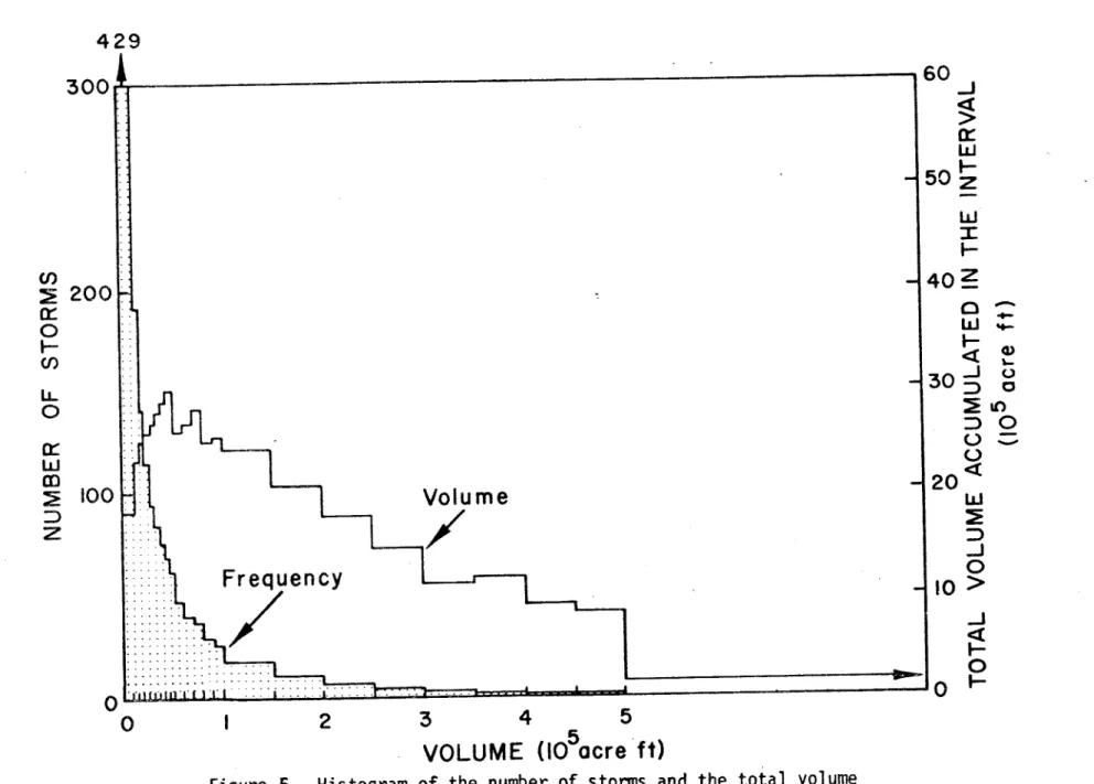
All precipitation events were included in the formation of storm events. The storms were partitioned into categories by their volume.

The histogram of the frequency distribution and the total volume yielded for each volume interval averaged over all regions are presented

in Figure 6. The volume category ;s shown in the horizontal axis. The average value was used because all regions display approximately the same distribution over the categories. The values shown on the figure were adjusted because the intervals among categories vary. 196 storms have volumes greater than or equal to 0.1 x 105 acre feet but less than O. 15 x 105 acre feet. The total volume of water contributed by these 196 storms is 24.2 x 105 acre feet.· As the storm size increases, the frequency

decreases very rapidly, but the total volume increases until the storm

size reaches C.S x 105 acre feet. then it begins to drop off very slowly. To find a relationship between the two parameters~ the volume and frequency occurring in each category were accumulated beginning from the largest category. Each accumulated value was then divided by its respective total to find the percentage accumulated up to that category. The

429 • 60...J

~

0: W I-50z

L·

-::::::

~

::::::;. ...

:

""-1

o

;fll',",IU'" ( ) "" I ' " t " ..i. . . ' ,

o

I 2 3 4 5 5 .

VOLUME (10

acre

tt)

Figure 6. Histogram of the number of stonns and the total volume

in each volume interval averaged over six regions.

en ~ ~ 2001".

o

I-CJ)

ll-e

0:: W

m

~ IOOH:

=>

z

Frequency

/

Volume

~/

W :I: ~ 40 2 o~ W +-

1-'1-«

Q,) 30 -.J t-o ::> c ~.&n I N ::>0 . , . . j

U.:::.

I U 20

«

w

~ ::> ....J 0 10

>

...J

~

0 0

I-

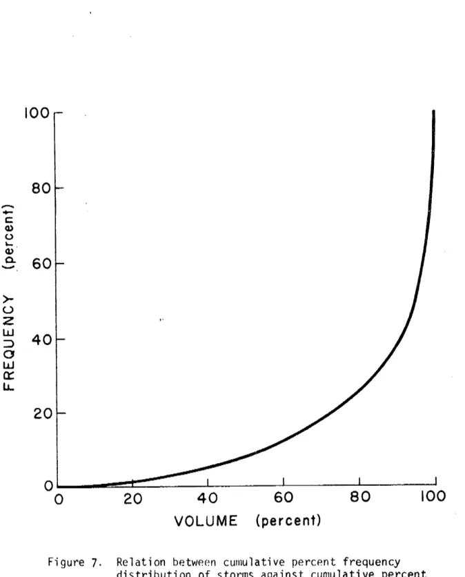
-22-regions is shown in Figure 7. Eighty percent of the storm volume is contributed by the largest 30 percent of the storm occurrences and 50

percent of the volume by about 10 percent of the storm events. In his analysis of Argentine rainfall, Olascoaga (1950) used daily precipitation data and obtained a simjlar curve.

The curve in Figure 7 "as very small slope at the lowest volume percentages and then increases very sharply. The point where volume ;s 83 percent was picked as the turning point because the curve appears to be fairly symmetrical there. This point was taken as the "noise level" where the largest categories which made up 83 percent of the total volume would be included in the analysis. They shall be referred to as significant storms. Even though about 70 percent of the storms would be ignored, the total volume included ;s sufficiently large to represent the precipitation regime.

To determine the validity of this "noise levelll

, the total monthly

volume was summed for four volume percentages: 100, 95, 83 and 55 percent. The monthly distribution of these volume percentages is shown in Figure 8. The 83 percent curve displays the monthly characteristics of each region

well enough to represent the precipitation regime.

4. 1 Starnl Characteristi cs

Referring to the significant storms (83 percent) in Figure 8, there are two distinct maxima for all regions except Region 5; one occurs in spring around March-May, and another in July and August. The maximum precipitation in early spring usually comes in the form of snow associated with large scale systems. It is a transitional period between winter and summer where the general circulation still retains some wintertime

-23-100

80

~ +-c Q) 0 ~ (1) a.

60

...,

>-u

z

w

40

::> 0 lJJ et:: La..

20

OL.-_.-!!~~--_L-_-_L-.._-_L..-_ _- J

o

20

40

60

80

100

VOLUME (percent)

Figure 7. Relation betwe(~n curnulative percpnt frequency distribution of storms against cunlulative percent storm volurne. Large size storms are cunlulated first.

"

..." \ -.t. 25 25 . 25

\

~ c:: ,... ~ ...

\

n> _Q)

00 "t0o-Q) 20 Region / 20 Region 3 20 I \

\

Q)

\

~ '-.. 0 0 I~ 0 15 15 - fa 15

I

\

\

lO I J \ :::s-f

«'

0 10.. _10I- 10t- 1/ V _{,~ 10} ~. w .... l~ _~ f'~_{--'. ::>} - J0- _..J 5t-~ ~" , . ' , V"" 5t- ... : \ 5 U'lCX>Oc: wWOc-+ 0 ~ ~ ~-J.

_>

0 ooo~ -t')-t}--f) 0' I I " , • • I I I • • O' • • • • • _{I I I} I I I I 0 0 JFMAMJJASOND JFMAMJJASOND QJOJQJ-t, - - ' - - I - " J ,. I --'-~ --' < N 0 1_\ J \ +::-V 1 +::-V l +::-V l - l ~ 20r 20r 20 I M'n-c-+c Region 2 0 _ _ : . - _ A 0 0 0 3 '~~(j) Q) 3 3

...

VlV)(/)-t, 0 Q) 15t- 15

r-

I 15 ...-.... _-s ~ \ (I) 0 -.J. _{OJ 0} <.0 ~ _to ~ ....d ~. 0 lOr \ \.. -...j~ 10~ " \'-10 -+» """S

-

....-"\ I ...." ('[) ...-n (Q W OJ

...

::s 0 _~ M- ;::) 5t- '. .' \ \'v/ , 5t-J: \

-,

.". _\~ 5 Vl :::> (/) -' ("'f-a 0 ~

>

_0' I I " f I I I I , I I 0.1 I , . , I I I I I I J ₀ V')

' - " JFMAMJJASOND JFMAMJJASOND JFMAMJJASOND

-25-precipitate heavily over a wide area. In late summer, the precipitation maximum is associated with thunderstorm activity. Regions 5 and 6 are the eastern plains with approximately the same rainfall characteristics of dry winters and wet summers. Region 5 has more precipitation than Region 6, and there is only one summer maximum as compared with two in Regions 6. This maximum in Region 5 occurs in May and lasts through August. In Region 6, the first maximum occurs in May followed by a

minimum in June, then another maximum of approximately the same magnitude occurs in July and August.

4.2 Seasonal Comparison

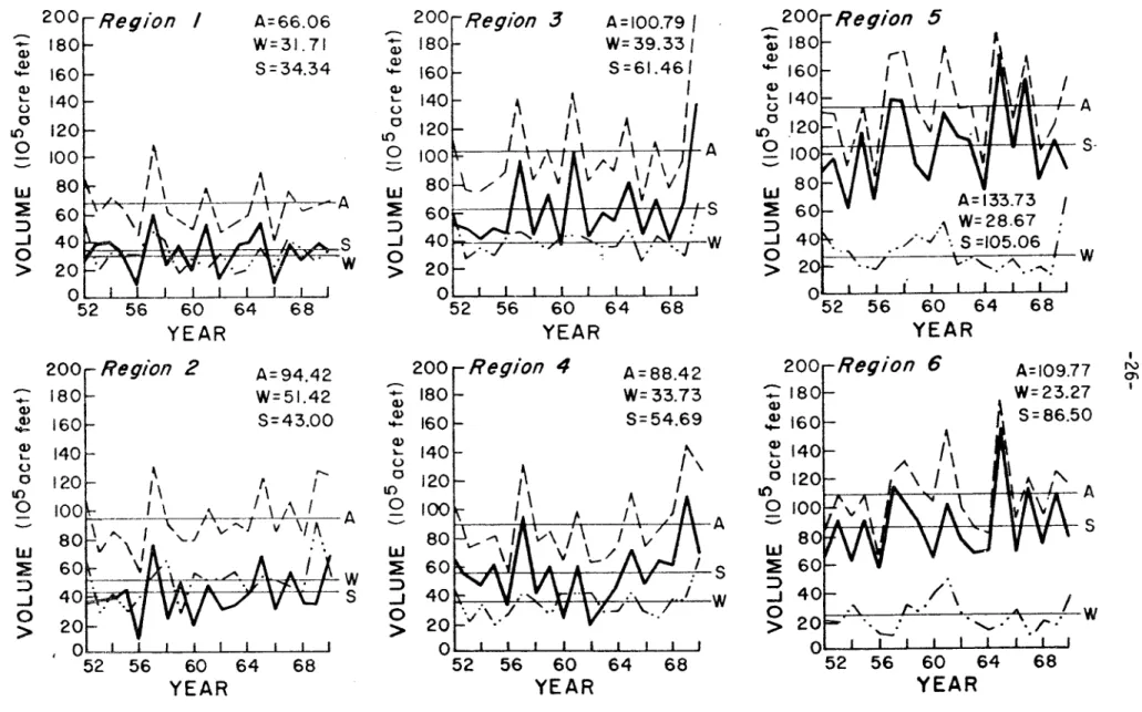
A

time series of annual, winter and summer precipitation volume for 1952-1970 is shown in Figure 9 for each region. Here the precipitation year begins in October of the previous calendar year and continues

through September. The annual volume is better correlated with the summer volume than with the winter volume. This correlation is illustrated by

the summer curves in Figure 9 where wet summers coincide with wet years. In Region 2, the winter-annual correlation coefficient is 0.63. It;s only eight percent below the summer correlation coefficient. Wet winters

occurred for this region in 1952, 1958 and 1969. In 1952 and 1969~ the annual values agreed with the winter value; whereas in 1958, the wet winter only compensated for the dry summer to yield an average year. The winter precipitation in Region 2 contributes 54 percent of the annual total precipitation. In the other regions, the summer months contribute more water to the annual total than do the winter months. The difference between the two seasonal correlation coefficients becomes correspondingly larger.

I

56 60 64 68

YEAR

200rRegion ~ 180 cv ~ 160

~

140L

'n'l

'-I"'':t'"

I A o I ( _ 10°

_o

.120. \_fOO~1'A'" \ I :,,\'.'1 '\h\

s-I ...

w

80 :E 60 ::> -I 4 0 . , . I W

o

_>

₂

or'

_'.7 _. t· ... "'\ ... '_{. , ' ,. "} .. .

.

. °52 A=IOO.79

I

W= 39.331 5=61.461 I I

.. . I

A=66.06 W=31.71 5=34.34 J I I I ...L-J 56 60 64 68

YEAR

Region I

200 ~ 180 Q) (l) 'to- 160 Q) ~ 140 ID O 120 o 100 W 80 lIIlIIl;;: ~- I ' I ' , \ -, .. ~ 60 f -::> -I 40~

1

~& I~ ,.,~. ·

o

~ ~ ~L ·~.S

>

20

--.rtf ..

;:)1=7. J

.~~ :w

o 52 I N 0"\

,

A=I09.77 W=23.27 ~ 5=86.50

'-""'.,;..!

w

/ ' \ 56 60 64 68

YEAR

Region 6 J. ... f A . • • IA' 'a A • At A \ . . . I . ~. ~ S w ~ ::> -I

o

>

A=88.42 W=33.73 5=54.69

i\

I J 64 68 A=94.42 W=51.42 5=43.00 "" " I ~\ / \ /\ I \---, "-~- ._~ -,-1 v

JV\/~A

..

,

I \ 56 60 64 68

YEAR

Region 2

I - - fL' \ .. '- r I'''~ / " W - 5 +-Q) Q) '+-w ~ :,) ...J o

>

Q) L. o o 10 o

Figure 9. Time series of the annual and seasonal total volume of 19 water years, 1952-1970.

A

=

Average

W

=

Winter

S

=

Sunmer

-27-The coefficient of variation is used to measure the relative variability of precipitation. Referring to Table 6~ the coefficients of variation in Regions 5 and 6 are lower for summer than winter where summer precipitation accounts for 80 percent of the annual volume. This low coefficient of variation for Regions 5 and 6 in the summer is primarily due to the large total summer precipitation volume. In the other regions, the coefficient of variation ;s lower for the winter season. The summer volume is 40 percent of the annual total in Regions 3 and 4 and 50 percent

in Regions 1 and 2. This suggests that the winter precipitation is less variable than summer precipitation. It also appears that the seasonal precipitation is more homogeneous in the north-south direction than in the east-west.

In spite of this north-south agreement among regions in the seasonal variation, the difference between winter and summer correlation coefficients is in better agreement in the east-west direction. The rlifference in

correlation coefficient ;s 0.24 in Regions 1 and 3 and 0.37 in Regions 4 and 6. A possible explanation for this agreement is that the storm track moves across Colorado in an approximate east-west orientation so that the storms affect the laterally adjacent regions in the same manner while reflecting the topographic characteristics of each region.

4.3 Event Analysis

In order to determine how storms of different yield affect the annual precipitation, storms were divided into five categories according to size. These categories are the same as those used by Riehl and Elsberry (1964).

The percentage of the volume in each class is shown in Table 7. Classes 1 and 5 yield approxin~telythe same amount of water~ about 14 percent of the total volume, and class 3 contributes twice that amount. The actual

-28-TARLE 6

..COr~PARISON OF VOLUME STATISTICS BETWEEN SEASONS.

EGIONS 1 2 3 4 5 6

-WINTER

.- h 31.71 51.42 39.33 33.73 28.67 23.27 v in 10:> acre ft. SO in 105 9.41 14.85 10.48 10.44 13.95 11.49 acre ft. I CV .30 .29 .27 .31 .49 .49 %of Annual 48 54 39 38 21 2" Precipe r .58 .63 .73 .53 .28 .56 SUl~iMER

v

in 105 34.34 43.00 61.46 54.69 105.06 86.50 acre ft. SD in 105 13.92 16~.32 26.08 21 .67 29.74 24.84 acre ft. CV .41 .38 .42 .40 .28 .29 %of Annual 52 46 61 62 79 79 Precipe r .83 •71 .96 .91 .89 .92

-ANNUAL

v

in 105 66.06 94.42 100.74 88.42 133.73 109.77 acre ft. SO in 105 17.04 20.99 32.69 25.29 30.39 25.54 acre ft.

I

CV .26 ' .22 .32 .29 .23 .23 --_._----~~

._._--_.

~·-~:_1.23-

~._-,._"--

- - - - -

---rsurn-rw;n .25 .38 .61 .36 R

~ ;s the average volume for the season SO

;s

the standard deviation

CV is the coefficient of variation given by

~

TABLE 7

CLASSIFICATION OF STORMS

Volume categories in 105 acre feet

%OF e-' _j for each region

i:

I

CLASS VOLU~1E FREQUENCY 1 2 3 4 5 6

I N U) .13 2 , ~5.4 >8.0 >6.8 >7.0 >12.5 >12.5 I

I

2 .22 9 5.3-2.7 7.9-4.4 6.7-4.0 6.9-3.8 12.4-7.2 12.4-6.5 3 .28 21 2.6-1.5 4.3-2.5 3.9-1.9 3.7-1.8 7.1-3.5 6.4-3.2 4 .23 29 -I 1.4-0.9 2.4--1.4 1.8-1 .0 1.7-1.0 3.4-1.7 3.1-1.7· 5 .14 39 I 0.8-0.0 1.3-0.0 0.9-0.0 0.9-0.0 1.6-0.0 1.6-0.0

-30-storm class varies for each region as shown in Table 7. In Table 8t the

number of storms that occurred in each category, the total volume and frequency and the average frequency for the driest and wettest five years averaged over the six regions are shown. In the last two lines of the table, it is shown that the driest quartile has two to three storms fewer than the wettest quartile for each of the categories; therefore, there does not appear to be a preferred storm size which ;s absent in a dry year. The omission of storms in a dry year appears to be approximately uniformly spread among all size categories.

The values in Table 8 were averaged over the six regions, thus smoothing out any irregularities in the frequency distribution. The actual frequency of storms over the categories from Region 6 is shown in Table 9. The third wettest year, 17, had 50 storms compared to only 38 storms for the wettest year, 19. Referring back to Table 7, five or six small class 5 storms are needed to compensate for the volume due to the lack of occurrence in large class 1 storms; whereas only two or three are needed to compensate for a medium size class 3 storm. Year 17 did not have any class 1 storms, but i t was compensated by the frequent occurrences in classes 3, 4 and 5 whereas year 11 had only 20 storms, ten storms fewer than its neighboring rank. Year 11 had its share of large storms~ yet lacked in the lowest three categories. Therefore, the annual volume is dependent on both the number of storms and the distribution of these storms among the yield categories.

Riehl and Elsberry found that the greatest contribution to the rank order of the annual precipitation total is obtained from the middle three classes of storms. The volume of precipitation contributed by the

TABLE 8

FREQUENCY OF STORMS BY CATEGORY FOR

EACH

YEAR

AVERAGED OVER ALL REGIONS RANKED BY VOLUME.

Annual Storm Volume Class Number and Percent Frequency in Each Class Total Number

Year _{5 1 2 3 4} "5 of Storms 10 acre feet 13% 22% 28% 23% 14% ~ 1 62 0 2 6 10 13 31 2 70 0 2 8 10 14 34 3 73 1 1 7 - 12 14 36 4 76 0 2 8 14 12 36 5 82 1 3 7 14 12 37 6 84 1 3 9 11 15 38 7 87 1 3 9 12 16 40 I 8 89 0 3 9 14 16 42 --'w 9 91 0 5 8 14 14 41 I 10 93 1 3 10 13 15 41 11 96 2 3 7 11 14 37 12 98 1 4 8 13 14 41 13 104 2 4 8 14 13 41 14 110 1 5 11 13 12 41 15 116 2 4 10 16 14 45 16 123 2 5 10 14 14 45 17 130 2 4 11 16 16 50 18 ₁₃₈ 3 5 13 14 16 50 19 157 3 9 9 15 15 51 Average frequency .4 2 7.2 12 13

driest five years

Average frequency 2.4 5.4 10.6 15 15

TABLE 9

FREQUENCY OF STORMS BY CATEGORY FOR EACH YEAR

RN~KED BY VOLUME FOR REGION 6

Annual Storm Volume Class Number and Percent Frequency in Each Cl~ss Total Number

Year ₁₀5

acre feet . 1 2 3 4 5 of Stonns

13% 22% 28~ 23% 14% 1 67 0 2 3 6 13 24 2 82 1 0 3 -: 11 12 27 3 85 1 1 6 12 9 29 4 86 1 1 4 14 7 27 5 93 0 2 8 14 4 28 6 94 0 3 10 4 10 27 7 94 1 3 6 7 9 26 wI 8 100 0 3 6 13 16 38 NI 9 . 105 0 4 7 13 9 33 10 110 0 3 11 9 14 37 11 110 1 3 7 4 5 20 12 114 1 4 8 7 12 32 13 115 0 4 8 14 9 35 14 12l 0 4 11 11 12 38 15 124 2 3 6 13 11 35 16 125 2 3 4 14 14 37 17 134 0 2 9 18 21 50 18 154 2 3 12 11 17 45 19 173 2 6 4 8 18 38 Average frequency .6 1.2 4.8 11 .4 9

driest five years

Average frequency 1.8 3.4 7 12.8 16.2

-33-Any difference in volume resulting from this class may easily be compensated by other classes (see year 11, Table 9). The occurrence of a large t class 1 storm would definitely increase the annual volume, but its average

frequency for the wettest quartile is only 2.4 per year which may easily be compensated by five to eight storms from class 4 or three to four

storms from class 3. Therefore, this confirms that the sum of the middle three categories is the most stable indicator of the "wetness" of a

certain year; the middle three categories account for an average of 70 percent of the annual precipitation.

The cumulative volume and frequency relationship for all the

significant storms is shown in Figure lOt curve A. The same relationship is shown in curve B as found by Olascoaga (1950) in his analysis of

Argentine rainfall and in curve C by Riehl and Elsberry·s (1964) analysis of the upper Colorado River Basin. These three curves agree with each other quite well. As Olascoaga pointed out, this relationship is

independent of geography and rainfall regime, i.e., the percent of storms yielding the middle 70 percent of the total volume is approximately the same independent of geography. Therefore, this middle 70 percent would also best indicate the "wetness" of a year _{for all regions in Colorado t} and other locations where the same graph holds true.

5. APPLICATIONS

This report presents background precipitation data for the state of Colorado as a whole and for six subregions. These data will be useful for the following applications. They provide a detailed description of the meteorological regimes responsible for the annual precipitation.

They provide a data base for Colorado land and resource planning and

-34-Ol...:l~:..-..JL..-_--'---""'--"""'----'

o

20

40

60

80

'100

PRECIPITATION (percent) 100 A

>-(..). ~ 40

~

8 w Q: 20

u.

-:: 80 c: Q) o '-Q) ~ 60

Figure 10. Percent cumulative storm volume versus percent cumulative storm frequency.

-35-trend. Already, J. Michael Sinton, a water resource engineer, and Harold W. Steinhofft the southwest regional administrator of the CSU

Cooperative Extension Service, have shown keen interest in the results of this project.

6. SUMMARY

It was found that no statistically significant trend, in the statewide precipitation for a 56 year period could be detected. When data from adjacent stations were analyzed, it showed that single stati~n precipitation data may be used to realistically represent an area average precipitation value. The characteristics of precipitation events of different sizes were computed and analyzed in detail from a 20 year set.

The annual precipitation of Colorado is produced by large scale

disturbances in the winter and by thunderstorms in the summer, and 80 percent of the precipitation volume is produced by 30 percent of the storm occurrences. The average storm duration is greater

for

the mountainous regions, and the volume of precipitation in the summer ;s better correlated with the annual volume than is the winter volume in all regions.

-36-REFERENCES

Draper, N. R. and H. Smith, 1966: Applied Re~ression

Analysis.

Jorn Wiley and Sons, In.

Henry,

A.

J., 1919: Increase of Precipitation with Latitude. Mon. Wea. Rev., 47, pp. 33-41.

Landsberg, H., 1969: Physical Climatology. 2nd Edition. Gray Printing Company, Inc. DuBois Pennsylvania, 446 pp.

Marlatt, W. E. and H. Riehl, 1963: Precipitation Regimes

Over

the Upper Colorado River. ~~ Geo~~__Res._t Vol. 68, No. 24, pp. 6447-6458. Olascoaga, M. J., 1950: Some Aspects of Argentine Rainfall. Tellus,

~, (4), pp. 312-318.

Riehl, H.,and R. L. Elsberry, 1964: Precipitation Episodes in the

Upper Colorado River Bas;n. Pure and Apple Geophys., ~, pp. 213-220. Sellers, W. D., 1960: Precipitation Trends in Arizona and Western New

Mexico. Proceedings of the 28th Annual Snow Conference, Santa Fe, New Mexico, pp. 81-94.