CO
A T d th in e p r in th l r o K r J Cent SE-1 SweESTIMA
ONNECT
Abstract The producti during the la hese estimat nfrastructure economic im production fu region – usin nput choices he infrastruc evel. The sig robustness of of trips acrosKeywords: Fi
region, Olley
JEL Codes: R
tre for Tra 100 44 Sto eden
ATION O
TION WI
A P
ivity of pub st two decad tes have been e stock, and mpacts of the functions fro ng a novel m s and self-sel cture, access gn and signi f the accessib ss Öresund. irm perform y and Pakes. R11, R15, H5 ansport Stu ockholmOF ACCE
ITH THE
PANEL O
Tom CTS Work lic infrastruc des, often wit n the level of d endogenei Öresund fix om firm data method due to lection into a ibility to the ificance of th bility parame ance, agglom 54 udiesESSIBIL
E ÖRESU
OF MIC
m Petersen – K king Paper cture has be ith vastly diff aggregation ity bias. In xed link, thes
a in Scania o Olley and account. As e workforce he two sour eter with resp
meration, ma
LITY EL
UND FIX
RO-DAT
KTH r 2011:10een the subj ffering result n of the data an attempt se issues are – the Swed Pakes (1996 a measure o is used on a ces of bias a pect to the sp arket potentia
ASTICIT
XED LIN
TA
ect of nume s. Matters of a, the measur t to estimat addressed b dish part of 6), that takes f the service a fine-grained are tested, as pecification o al, accessibilTIES IN
NK USIN
erous studies f concern for rement of the te the wider by estimating the Öresund s endogenous e provided by d geographic s well as the of the barrier lity, ÖresundNG
s r e r g d s y c e r dEstimation of accessibility elasticities in
connection with the Öresund …xed link using a
panel of micro-data
Abstract
The productivity of public infrastructure has been the subject of numer-ous studies during the last two decades, often with vastly di¤ering results. Matters of concern for these estimates have been the level of aggregation of the data, the measurement of the infrastructure stock, and endogeneity bias. In an attempt to estimate the wider economic impacts of the Öresund …xed link, these issues are addressed by estimating production functions from …rm data in Scania— the Swedish part of the Öresund region— using a novel method due to Olley and Pakes (1996), that takes endogenous input choices and self-selection into account. As a measure of the service provided by the infrastructure, accessibility to the workforce is used on a …ne-grained geographic level. The sign and signi…cance of the two sources of bias are tested, as well as the robustness of the accessibility parameter with respect to the speci…cation of the barrier of trips across Öresund.
Keywords:Firm performance, agglomeration, market potential, accessibil-ity, Öresund region, Olley and Pakes.
1
Introduction
The productivity of public infrastructure has been the subject of hundreds of studies since the 1970’s with a surge in the 1990’s after the publication of Aschauer (1989) and the following debate (Munnell, 1990, 1992; Tatom, 1991, 1993).
The motivations behind this interest are partly to provide guidance for policy decisions, for example as input to cost-bene…t analysis of so-called “wider e¤ects”, partly to understand the complex role of infrastructure and in the economy, and (more recently) to provide evidence for theoretical models in new economic geog-raphy, new growth and new trade theories. The literature on the e¤ect of public infrastructure started as an attempt to explain the productivity slowdown in the
US economy from the 1970’s and onwards. For comprehensive reviews of this liter-ature, see for example Gramlich (1994); Sturm, Kuper, and de Haan (1998); Romp and de Haan (2007); Mikelbank and Jackson (2000); Lakshmanan (2010); Straub (2008); Bell and McGuire (1997).
About a decade earlier, as a consequence of a decline in the population in large metropolises, the economies of city size were examined and speculations about the “optimal size” of cities were formed (Mera, 1973). This gave rise to a rich theoretic and empirical literature trying to pin down the foundations and forces of agglomeration economies.
In two recent meta-analyses, the number of studies considered were 67 about the private output elasticity of public capital and 34 about agglomeration exter-nalities (Melo, Graham, and Noland, 2009; Bom and Ligthart, 2009), and these numbers are not exhaustive.
Bom and Ligthart (2009) estimate the short-run output elasticity of agglom-eration, corrected for bi-directional publication bias, to 0.085 and the long-run elasticity to 0.27, but with a large heterogeneity among estimates. They report that the main reasons for the heterogeneity are: the empirical model, estimation technique, the type of public capital and the level of aggregation of the public capital data. They …nd the long-run elasticity to be consistent with the earlier time-series estimates, and that the “primary”(uncorrected) elasticities are signif-icantly in‡ated by publication bias. Melo et al. (2009) question why one would expect the same elasticities in
Early time-series studies were based on the total US economy or federal state economies, but later on it became more common with smaller geographical divi-sions: county or metropolitan areas. The econometric problems facing these esti-mations are manifold, but the most important are perhaps endogeneity of input choices, missing variables, spurious regression, spatial autocorrelation and mea-surement error. Their respective seriousness depend, among other things, on the spatial and temporal resolution of the data.
Another review of agglomeration, with a focus on policy conclusions, is pre-sented by Gill and Goh (2010).
The construction of the Öresund …xed link provides a new opportunity to esti-mate the e¤ect of infrastructure on economic performance. The link connects two large markets, Copenhagen, the capital of Denmark with 1.8 million inhabitants (metropolitan area), and Malmö, the third largest city in Sweden with 0.52 million inhabitants (Greater Malmö area; population …gures are from Dec 31, 1999) and was opened on July 1st, 2000. In this paper, I present results from the estimation of agglomeration elasticities in production functions with disaggregated panel data (workplace/plant level), in the Swedish part of the Öresund region (Scania) before and after this major change in the infrastructure took place: between 1995 and
2004.
1.1
Estimation issues
Disaggregated panel data are increasingly being used for productivity analysis, because of its availability and its potential to gain new insights in the workings of the economy at the lowest level, which is important for e¢ cient policy making. These new data sources do however not necessarily solve the estimation di¢ culties of earlier studies on aggregate data, and might in fact introduce new ones. En-dogeneity is for example as important at the micro level as it is in the aggregate, although of a di¤erent kind. With micro data, endogeneity appears because of our ignorance about the internal information set of the management, about the market situation, future plans etc. Moreover, these unobservables are serially correlated, which is a major challenge to the econometrician.
The endogeneity gives rise to a skewed distribution of the errors, which biases the estimates, and serial correlation deteriorates the e¢ ciency of e.g. the OLS es-timator and biases the standard errors downwards, potentially leading to spurious rejection of null hypotheses. The endogeneity bias is also known as transmission bias after Marschak and Andrews (1944), because the unobservable productivity a¤ects input requirements, which are transmitted to the output. The usual meth-ods to cope with endogeneity and …xed e¤ects is instrumental variables estimation of some form, using transformed data (e.g. by …rst-di¤erencing, Within transfor-mation1, or the orthogonal deviations due to Arellano and Bover (1995)).
How-ever, di¤erencing in either form enhances measurement error and biases estimates towards 0 (attenuation bias, see Griliches and Hausman (1986, for example)).2
Another endogeneity and source of potential misspeci…cation is the fact that managers not only make decisions about how to continue the business, they also de-cide whether to discontinue it all together. For the econometrician, this is a source of self-selection or attrition bias in the data, if we assume that the decision to discontinue is not taken at random. Rather, this decision is based on performance indicators, accumulated capital, the reservation price of the business etc. Some of these can be captured through e.g. …nancial statements, while some–notably productivity and “inside information”— are inevitably hidden for the researcher. For overviews of how to handle the endogeneity issue, and all other aspects of pro-ductivity estimation on micro data, see Griliches and Mairesse (1995); Eberhardt
1Also called “Fixed e¤ects” estimation.
2In the generalised method of moments (GMM) framework, it is possible to take both
mea-surement error and endogeneity into account, although e¢ ciency could be an issue together with the problem of …nding the right set of instruments, and having time series of su¢ cient length (Griliches and Hausman, 1986; Arellano and Bond, 1991; Hansen, 1982; Blundell and Bond, 1998, among others).
and Helmers (2010); Syverson (2010); Gandhi, Navarro, and Rivers (2009)
The omission of relevant variables leads to bias in the estimated parameters if there is correlation between the included and the omitted variables, and be-tween the omitted variables and the dependent variable (i.e., they are “relevant”) (Greene, 2000, p. 334). Consider the regression
y= X1 1+ X2 2+ ;
where all terms are in vector format, and X1 and X2 are matrices with K1 and
K2 columns, respectively. Now if y is regressed on X1 without including X2, the
estimator is b1 = 1+ (X01X1) 1 X01X2 2+ (X01X1) 1 X01 :
Taking the expectation, the last term disappears and we get E [b1] = 1+ P1:2 2,
where P1:2 = (X01X1) 1
X01X2 is a K1 K2 matrix with each column being the
slopes in a regression of X2 on X1. Unless either X2 and X1 are uncorrelated, or
the true 2 0, b1 will be a biased estimate. Furthermore, the direction of the bias
is undetermined: it will depend on the combination of the sign of the correlation between the omitted and included variables, and the sign of the elements of 2
(i.e. the “true” slopes in a regression of y where X2 is included). If K2 > 1, the
bias will also depend on the correlation between the di¤erent omitted variables. It is also possible that the impacts of the combination of di¤erent variables in X2
and 2 cancel out, so that the resulting bias of b1 is close to 0. This fact might
explain why OLS sometimes seems to be a reasonable estimation method, while the background in‡uences to this result are concealed. In Table 5 I present the counteracting e¤ects of endogenous production and selection on the estimates of the agglomeration elasticity.
1.2
Aim of the paper and hypotheses
In this paper I want to examine the nature and size of the e¤ects of higher ac-cessibility on production in di¤erent industries. I also want to shed some light on the biases at work when these estimates are compared with ordinary least squares (OLS), caused by unobserved heterogeneity and endogeneous selection. I present estimates of production elasticities of accessibility on cross-sectional level, by 2-digit industry, manufacturing/service and for the whole regional economy. As a robustness check, the estimates are compared for three di¤erent levels of barrier across Öresund after the establishment of the …xed link. The OLS estimates are compared with estimates by the Olley-Pakes method and the e¤ect of the omit-ted information on past performance and . Finally, I use estimaomit-ted …rm-speci…c technical e¢ ciencies, aggregated by the small market area zones used for tra¢ c
analysis, and run regressions on 5-year growth to investigate the longer term con-nection between raised accessibility and this increase in “geographic”productivity (i.e. productivity by zones).
The hypotheses tested are thus:
1. There is no shift in cross-section production stemming from higher accessi-bility.
2. There is no bias in OLS estimates of accessibility elasticities.
3. There is no long-term e¤ect of higher accessibility on geographic productivity. The paper is structured as follows: the next section describes various aspects of the included variables, especially accessibility, followed by a section about the three-stage estimation procedure of Olley and Pakes. In this part a special subsec-tion is devoted to the survival model. After that, the results of both the survival and the production regression models are presented, and some results connected to the changed situation in the Öresund region. More detailed results for the goods and service sectors are attached in the Appendix.
1.3
Productivity, technical change and technical e¢ ciency
In general, total factor productivity (T F P ) is measured as the ratio of an index of output Y to an index of inputs X, or equivalently the di¤erence between their logarithms, where the indices are products or sums weighted by their respective output or cost shares (Bauer, 1990). For the production frontier function y = f (x; t), the one period Divisia index of T F P in logarithmic form is
T F P = ln y X
i
siln xi;
where si are the value shares of input (cost shares), i.e.
si = wixi C = wixi P iwixi ;
with factor prices wi and y and xi are volumes of output and inputs. In order
to represent the case where a …rm is not fully e¢ cient, in the meaning that it produces less than possible at a speci…c level of inputs, we can premultiply y with a factor = y=y , where y is now the production frontier, that is the maximum possible amount that can be produced with input vector x with period t technology (0 < 6 1) (Farrell, 1957). In logarithmic form we get
Di¤erentiating with respect to t gives : y = : +X i @f @xi xi f : xi+ : f = : +X i "i : xi+ : f
where dot above means growth rate, and "i is the output elasticity of input i. If
…rms are minimising cost, "ican be expressed as "si, with " =
P
i"i the elasticity of
scale, by homogeneity of the production function3. If production exhibits constant returns to scale, " = 1, and factors are paid their marginal product, then the technical production parameters "i equal the cost shares si.
Now
:
is the relative (“percentage”) change in technical e¢ ciency (T E) and
:
f is overall technical change of the industry (T C, a time trend), and "i are the
estimated Cobb-Douglas output elasticities. We therefore de…ne a suitable perfor-mance measure in log-levels, with T C speci…ed as a quadratic time trend:
ln = ln y X
i
i ln xi t t tt t2:
where -s are now parameters to be estimated. We thus assume constant returns to scale. In practice, since we are using a Cobb-Douglas speci…cation, this often yields scale elasticities close to 1 because of the inherent bias towards this value (see Hoch, 1958), so this performance measure will be close to any estimated productivity using this speci…cation.4
2
Data
2.1
Accessibility
The data can be divided in two sources: the data used for accessibility computa-tions and the …rm-speci…c variables. The accessibility calculacomputa-tions are made from population data and calculated travel times between zones in an irregular lattice of 1,345 zones. The geographical coverage is almost the whole Öresund region, namely Scania in Sweden and in Denmark, the entire Zealand plus Møn5. The
3Cost minimisation gives input prices w
i = @x@fi, with the Lagrange parameter . Multiply
with xi and sum over inputs to get C = f ": Now, "si= CfwCixi = @x@fixfi = "i:
4Note also that inversion-based estimators like the one of Olley and Pakes “ignore the
varia-tion in input mixes and/or measurement errors in inputs” (Gorodnichenko, 2007) and therefore estaimates of returns to scale (RTS) are biased. RTS is however not the main interest of this study.
5According to the de…nition of Statistics Sweden and Statistics Denmark, the Øresund region
also includes the islands Lolland, Falster and Bornholm, which are inhabited by 4.3 % of the total population in the region (Dec 31, 2005).
population measure we use is the population in working age, 16–69 years. Some of the data, especially on the Danish side, has been disaggregated from the municipal level onto the …ner zonal lattice, in order to take advantage of the travel times. The population data is divided into four classes of last ful…lled education, but this is not used in the present study. The travel times are computed by the SAMPERS travel demand model for work trips by car. Accessibility is computed as a so-called relative Hansen measure, which means that the attraction variable is the share of the population in each zone out of the region total every year. This avoids spurious e¤ects from growth in the total population later in the regressions.This attraction variable is discounted geographically by a declining function of travel time:
accrt= N X j=1 P OP 1669jt PN r=1P OP 1669rt e 0:038 T T Crjt;
where accrt is accessibility in zone r in year t, P OP 1669xt is the population
be-tweeen 16 and 69 years in zone x in year t, and T T Crjt is travel time by car
between zones r and j in year t. The discounting (impedance) parameter 0:038 is chosen so that with a travel time of one hour (expressed in minutes), there is only a 10 % probability that the population makes the trip, compared to the situ-ation with zero travel time. This is also the parameter used in TransCad6 for work
trips. Both accessibility and travel times are indexed by time, because the travel time across the Strait of Öresund changes dramatically in the year 2000, which a¤ects the accessibility in the whole area although the e¤ect is declining towards the periferies. This fact should provide a good foundation for the estimation of the accessibility elasticity, since it is varying in both the cross-section and time dimensions. In reality, only two matrices of travel times are calculated; before and after the …xed link is introduced. In the year 2000, since the opening was exactly in the middle of the year (July 1), a mean of the before- and after-travel times is used in each zone. The year-to-year variability of the accessibility measure is still guaranteed through the variations in population (which, however, are small in comparison). The accessibility variable is coded on each …rm/workplace by the geographical coordinates of the …rm.
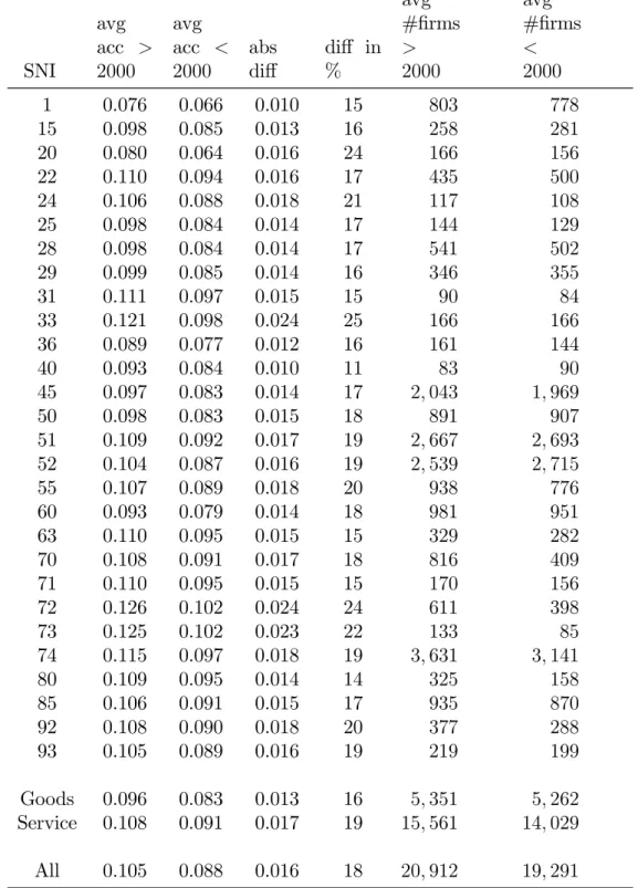
The changes in accessibility by industry are presented in Table 1. The base accessibility ranges from 0.064 to 0.102, with a weighted average of 0.088 (the overall average base accessibility level). The relative increases vary from 11 to 25 % between industries, with an overall average increase of 18 %. These are quite large increases, mainly due to the reduction in travel time to the Danish capital (a small portion depends on the population increase).
6TransCad is a Geographic Information System software for Transport modelling applications
SNI avg acc > 2000 avg acc < 2000 abs di¤ di¤ in % avg #…rms > 2000 avg #…rms < 2000 1 0.076 0.066 0.010 15 803 778 15 0.098 0.085 0.013 16 258 281 20 0.080 0.064 0.016 24 166 156 22 0.110 0.094 0.016 17 435 500 24 0.106 0.088 0.018 21 117 108 25 0.098 0.084 0.014 17 144 129 28 0.098 0.084 0.014 17 541 502 29 0.099 0.085 0.014 16 346 355 31 0.111 0.097 0.015 15 90 84 33 0.121 0.098 0.024 25 166 166 36 0.089 0.077 0.012 16 161 144 40 0.093 0.084 0.010 11 83 90 45 0.097 0.083 0.014 17 2; 043 1; 969 50 0.098 0.083 0.015 18 891 907 51 0.109 0.092 0.017 19 2; 667 2; 693 52 0.104 0.087 0.016 19 2; 539 2; 715 55 0.107 0.089 0.018 20 938 776 60 0.093 0.079 0.014 18 981 951 63 0.110 0.095 0.015 15 329 282 70 0.108 0.091 0.017 18 816 409 71 0.110 0.095 0.015 15 170 156 72 0.126 0.102 0.024 24 611 398 73 0.125 0.102 0.023 22 133 85 74 0.115 0.097 0.018 19 3; 631 3; 141 80 0.109 0.095 0.014 14 325 158 85 0.106 0.091 0.015 17 935 870 92 0.108 0.090 0.018 20 377 288 93 0.105 0.089 0.016 19 219 199 Goods 0.096 0.083 0.013 16 5; 351 5; 262 Service 0.108 0.091 0.017 19 15; 561 14; 029 All 0.105 0.088 0.016 18 20; 912 19; 291
Table 1: The average change in accessibility for the included …rms in the dataset, by industry, and the approximate number of …rms a¤ected.
The assumptions about the travel impedances are crucial for the accessibility measure, and thus for the estimation of production elasticities. The travel times for the passage over the Öresund Strait are fetched from the regional SAMPERS model (ref Beser-Algers), which was calibrated with regard to trips crossing the Strait. Therefore, the link times are not exactly as the actual travel times, but includes some extra time to account for di¤erent barrier e¤ects (which account for that travel is lower than ”expected“). These extra amounts also accounts for monetary costs, interchange and waiting times, inconveniences etc.
The passing time time it takes for a car trip from central Malmö to central Copenhagen according to the shortest path algorithm is 133 min before the …xed link (over the ferry link Limhamn-Dragør). After the …xed link opened, the travel time is 40 min. The service of the ferries between Helsingborg and Helsingør in the Northern crossing has not changed essentially. The monetary costs to pass the Öresund Strait are assumed to be approximately equal in real terms before and after the introduction of the …xed link. This is not unreasonable, since the pricing scheme is restricted by the governments not to exercise unfair competition towards the Northern part of the Strait7. In order to keep these extra impedances as much as possible, we assume a mean waiting time of half the service interval, as is usual in modelling practice, and calculate the extra impedance in MC to 101 (55 + 60=2=2) = 31minutes, which is added to the driving time on the …xed link, approximately 10 minutes coast-to-coast.8
2.2
Firm-level data
The …rm-speci…c variables are compiled from the …nancial accounts of all …rms except self-employed, and are obtained from Statistics Sweden for the years 1995– 2004 (as of Dec 31 each year). The industrial coverage is the primary sector, man-ufacturing and service industries, except the …nancial sector (banks and insurance companies). Due to our need for a well-de…ned geographical location, …rms with several workplaces inside Scania are excluded, and only …rms with more than 50 % of their activity in terms of number of employees work there are included. This se-lection rule might bias the results, since …rms with more than one plant/workplace ar likely larger than single-unit …rms. On the other hand, the number of single-unit …rms is massively dominating the number of multi-unit …rms: the average number of workplaces per …rm in 2004 was 1.087 in Sweden. But worse, this selection rule is active in all time periods, meaning that if a single-unit …rm is transformed into
7Except the Limhamn–Dragør line, which carried motorised vehicles, there was a shuttle
between central Malmö and the Kastrup airport (Flygbåtarna), but since we calculate car travel times this is not included in the model.
8In the HH crossing it is 78 (25 + 60=4=2) = 45: 5 minutes, although it is not used since we
coast-to-coast between city centres model real approx. freq. per hour before 2000 after 2000 before 2000 after 2000 Helsingborg– Helsingør 25 4 78 85 est. A 25 32 est. B 49 56 est. C 78 85 Malmö– Copenhagen, via Limhamn–Dragør 55 2 101 – 133 via …xed link 10 –
est. A 10 42
est. B 34 66
est. C 41 73
Table 2: The real and implemented passage times for accessibility calculations, in minutes.
a multi-unit one, for example through merger or acquisition, it drops out of the dataset in that time period; and conversely, if it sells o¤ a unit, it can reappear. However, there is no workaround for this, because …nancial accounts are made for …rms and not workplaces.
On the other hand, groups of companies are represented if their members are autonomous, single-plant …rms; this is the case for some grocery chains and franchises, for example. However, groups of companies potentially pose other problems to data management and estimation, since they have the possibility to redistribute certain pro…ts and assets between its members. In order to avoid this, I have used performance measures that are independent of such transactions (such as for example earnings before …nancial entries and balance-sheet allocations).
Variables on production, investment, capital and value-added are transformed into volumes by industry-speci…c cost indices. Dummies for start-up and closures of plants, change of location, change of activity and change of owner category are coded from the time series of the id-s, location variable, activity code and own-ership class (e.g. public, private or foreign) from the unbalanced data set. The dummy for start-up is constructed from the age variable and available for all years. The dummy for closure is constructed from the last observation of each work-place id, which in a way could be misleading since id-s could change for other reasons than closure (for example change of owner or activity). However, it surely indi-cates that ”something happened“ in this year, and for example change of activity is already captured through its own dummy. The closure dummy is of course un-available in the last year of the panel. The change of location is constructed from changes in coordinates that are not caused by missing geographical coding.
The measure of capital is the book value of capital, and not the perpetual inventory used by many other authors. With the book value method, last years capital is depreciated by actual monetary values of depreciation and this years (net) investment is added, while the perpetual inventory method adds lagged capital, depreciated by a …xed percentage, to current year investment. With both methods restrictive assumptions have to be made about the depreciation in the “real”value of the capital stock to the …rm: for example, depreciation rate, vintages, utilisation rate, adjustment costs, etc. The book value method is used here for simplicity. Besides, there are empirical results indicating that it might be more appropriate to appreciate the value of capital in the years following an investment, due to gestation lags (Pakes and Griliches, 1984).
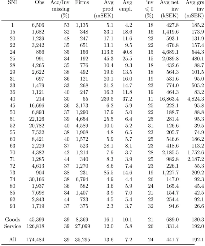
In Table 9 in the Appendix, some summary statistics for each 2-digit industry are presented, as well as for the aggregate goods and service sectors and the whole dataset. It is apparent that the industries are quite di¤erent in terms of number, output, average employment and investments, and this should always be kept in mind when analysing them all by more or less the same method as we do
here. Note that the unit of gross invesment in the right-most column is 1,000 times greater than the one for net investment. It is also shown that a great deal of observations are lost by both lacking location information (no accessibility observation) and the restriction we have on investment: on average around 40 % missing. Apart from them, all …rms with more than one unit are excluded because of their locational ambiguity. The size distribution of the …rms in the dataset, as compared to the distribution in Sweden, is shown in Table 3. There is quite good agreement of the distributions up to sizes of 100 employees–above that, the sample is underrepresentative. Whether this depends on regional di¤erences or if it is a “true” underrepresentation is not known.
#employees Sweden (%) Scania dataset (%) 0 75 1-4 17 68 66 5-9 4.0 16 18 10-19 2.1 8.3 8.7 20-49 1.2 4.8 4.7 50-99 0.4 1.4 1.4 100-199 0.2 0.7 0.4 200-499 0.1 0.4 0.2 500+ 0.1 0.4 0.1
Table 3: The size distribution of …rms in Sweden and in the Scania dataset as of Dec 31, 2004. The two rightmost columns show the distributions of non-self-employed …rms, which is the relevant one in this dataset.
For details on the average sizes of …rms in the sample compared to the Sweden average, see Table 4. In 2004, the average size of …rms in Sweden excluding self-employed was 6.5 employees. For the “goods”industries (SNI 1–45) it was higher, 11.5, and for the service sectors (SNI 50–93 except for the …nancial and insurance sectorsc: SNI 65–67) it was 5.0. If electricity, gas, and water supply (SNI 40–41; 20.2 employees/…rm) and construction (SNI 45; 4.7 employees/…rm) are excluded from the industry sectors, the average size in 2004 rises to 18.7 employees/…rm in the remaining goods industries. For the whole period 1995–2004, the average size in goods (except electricity generation and construction, i.e. in SNI 1–37) was 21.5, and in services except …nance and insurance 5.3. The all together average size in these industries (SNI 1–37, 50–63 and 70–93) was 7.5. (Note that these two
2004
without SNI 40–45 Sweden Scania sample Sweden Scania sample Goods 11.5 11.5 18.7 14.5 Service 5.0 6.0 5.0 6.0
All 6.5 7.4 6.7 7.5 avg. 1995 2004
without SNI 40–45 …nal sample (Table 9) Sweden Scania sample Sweden Scania sample
Goods 11.9 21.5 14.9 10.1
Service 5.3 5.8 5.3 5.8 5.8
All 7.5 7.5 7.6 7.2
Table 4: Average sizes of …rms in Sweden and in the Scania sample. samples are not entirely comparable.)
In my sample from Scania, the overall average size for the whole sampling period is 7.2 employees/…rm for all …rms (including electricity generation and construction), for the “goods” sectors, including electricity generation and con-struction, 10.1, and for the service sectors except …nance and insurance 5.8 (see Table 9 in the Appendix). Thus, only in the goods sectors the average size is slightly di¤erent from the Sweden average. However, this could at least partly be attributed to regional di¤erences: most of the largest companies in for example mining, steel production, paper and pulp production and car and truck manufac-turing are located outside Scania.
The manufacturing industries in Scania are dominated by companies in the food and packaging industries (Tetra Pak, Alfa Laval, PLM), rubber and chemical industries (Trelleborg, Perstorp, Boliden Kemi), telecommunications (Sony Eric-sson) and medical equipment (Gambro). Other large companies in the “goods” sector are E.ON (electricity supply) and Skanska and PEAB (construction).
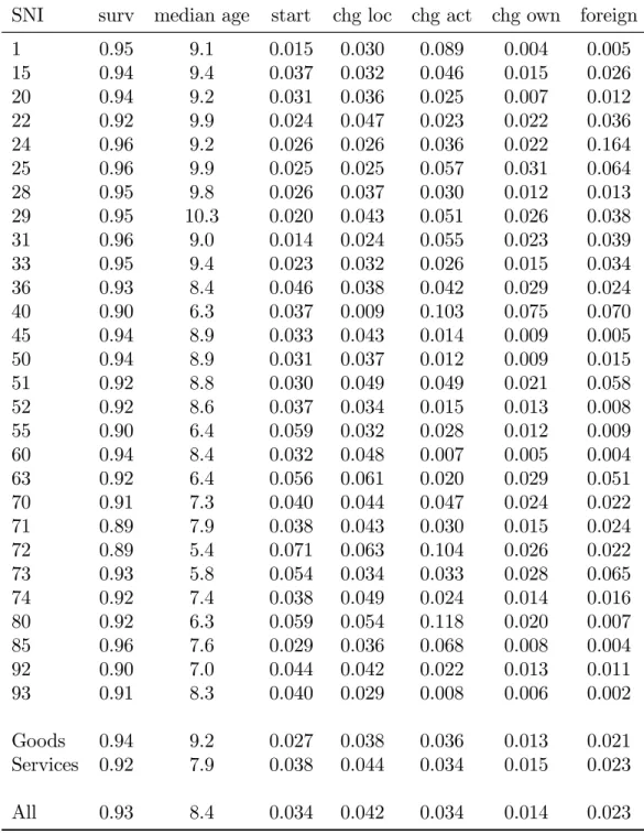
In Table 10 in the Appendix, some of the dynamic properties of the indus-tries are listed in grand averages: survival from year to year, frequency of starters (entry), relocation, change in activity code (5-digit SNI) and change in ownership category (not ownership in itself). The ownership categories are only a few: pub-lic, private without and with group association, or foreign ownership. The rate
of foreign ownership is also included. It is immediately visible that for example the survival rates are lower, and the entry and relocation rates are higher in the service sector, while the propensity to change activity or ownership category are about the same, although they vary a lot across two-digit industries.
2.3
Censored age variable
The age variable is calculated from the start date of the …rm, which is censored to the left at Dec 31, 1971. This in turn means that age is censored to the right at between 24 and 33 years, depending on the year. It also means that age is expressed in fractions of years, if it started somewhere in the middle of the …rst year. The censored proportion varies from 1 to 51 %, depending on the mean age of the industry, and decreases naturally along the period. In general, industries with high entry and exit rates like Hotels and restaurants and Other business activities, are those with the lowest median age and also the lowest proportion of censored observations. Censoring in the explanatory variables is essentially a missing-value problem, which mainly a¤ects the estimation e¢ ciency, but if age is correlated with the unobserved idiosyncratic e¤ects (i.e. not missing at random), it can also generate bias. This could be mitigated by imputation. However, although there are methods for this in the duration model literature (Pan, 2001; Hsu, Taylor, Murray, and Commenges, 2007), in the case of censoring this is not trivial, because the imputation must be made outside the range of the variable in question according to some hypothetical distribution. Instead I have chosen to exclude the censored observations.
3
Estimation
3.1
Olley-Pakes estimation
In the estimation approach of Pakes (1994) and Olley and Pakes (1996), both sources of bias are accounted for. Two ”helper functions“ are estimated— one accounting for the transmission bias and the other for the self-selection bias— together with the parameters of interest, and predictions from them are included in a ”bias function“ in the last stage. The bias function is approximated as a Taylor series expansion (polynomial series) of the two helper functions.
The framework for estimation of the parameters in the production function is explained in detail in Ackerberg, Benkard, Berry, and Pakes (2007, sect. 2.3).9 It 9It has been extended by Muendler (2007) to allow for negative net investments, and by
provides a method for taking account of persistent unobserved …rm heterogene-ity, which induces serial correlation, and endogenous (self-)selection. A …rm is supposed to enter the market by investing an entry fee in order to test the com-petitiveness of its speci…c entrepreneurial idea. Once in the market, in each time period the …rm calculates its expected discounted future returns V (!t; kt; at; Dt),
conditional on its e¢ ciency level !t, capital endowments kt, age at and a vector of
market or environmental conditions Dt. These market conditions are common to
at least some of the …rms in the market and could include for example input prices, output market characteristics, industry structure, technology, tari¤s, regulations, weather etc. In this speci…c application it also includes the accessibility in the zone where the …rm is located. The reason for bringing age into the value function is to separate the cohort e¤ect from the selection e¤ect in determining the impact of age on productivity (Ackerberg et al., 2007).
The …rm compares this value with a reservation price (sell-o¤ value) t =
(!t; kt; at; Dt), and if it is less than that it takes t and exits from the market.
It controls the value of its future e¢ ciency level by investments N etInvV olt 1,
which increases capital deterministically. In terms of productivity, the returns of the investment is stochastic and follows a …rst-order Markov process:
p !jt+1j f!j g t
=0; Jjt = p (!jt+1j!jt)
where Jjt is the total information set in period t, that is all previous values of
all variables from the beginning up to time period t. This equation states that productivity in t + 1 only depends on productivity in t, regardless of past history (history is assumed to lead to accumulated knowledge and other factors determin-ing productivity, all available in t).
The Bellman equation for an incumbent …rm becomes Vt(!t; at; kt; Dt) = max N etInvV olt; tf t; sup N etInvV olt>0 [ t(!t; at; kt; Dt) c (N etInvV olt) + + E (Vt(!t+1; at+1; kt+1; Dt+1)jJt)]g (1)
where t is the discrete control to continue in operation (if t= 1) or to exit from
the market and collect the sell-o¤ value t ( t= 0), and the discount factor is the
constant . This is the conceptual framework for a …rm with state variables k and ! solving a dynamic programming problem using the control variables N etInvV ol and ; but we will not attempt to solve for the valuation function in (1); instead, we side-step this rather cumbersome problem and focus on the removal of the most important biases mentioned above.10
The …rm is assumed to know the level of all (slowly adjusted) state variables (productivity, capital, age and market conditions) in the beginning of each time period, while inputs of intermediate goods and labour are assumed to be adjusted during the whole time period, as a response to exogenous shocks and changes in the environment D. These inputs are termed “non-dynamic”, since they only a¤ect production in the current time period. The case is di¤erent for the investment control: it is known one period in advance, and a¤ects the production in following time periods (and is thus “dynamic”). This also means that we assume that it takes a full time period (one year) to order, receive and install new capital before it can be productive.
Besides this “timing”assumption, there are two other assumptions in this esti-mation strategy: …rst, …rm performance, unobserved by the researcher but at least partly known in advance by the …rm management (because of serial correlation), is assumed to vary positively and monotonically with investment, at least for …rms whith strictly positive investment11. Second, productivity is assumed to be the
only unobserved state variable. The whole idea is to account for the “insider infor-mation” of the management of the …rm by looking at its actions, viz. investment decisions. If the management has high expectations about its …rms possibilities in the future market, then it invests, and the higher the beliefs, the larger the amount of investment.
The optimisation problem in (1) results in two decision rules, one for each of the controls:
t=
1 if !t> !t(ln kbt; ln kmt; aget; ln acct)
0 otherwise ;
and
N etInvV olt= N etInvV ol (!t; ln kbt; ln kmt; aget; ln acct) ;
where !t( ) (the lower limit of productivity before exit) and N etInvV olt( ) are
determined by the market equilibrium in period t, and depend on all the variables determining that equilibrium, including e.g. input prices, industry structure, etc. Given the monotonicity (for N etInvV ol > 0) of the scalar productivity !, we can invert the investment control function N etInvV ol = N etInvV ol (!; D) and
e¢ ciency and market prospects, making investments necessary to stay in business. There is also a continuous entry of new …rms which contribute to the market structure and thus the level of competition at each stage in the development of the business (Ericson and Pakes, 1995).
11Although this has in theory been relaxed in the studies by Muendler and Levinsohn and
Petrin (2003). However, empirical results from this study do not support monotonicity for negative net investments (i.e. disinvestments greater than or equal to gross investments in one year). Rather, it seems that a high level of productivity implies both high levels of investment and disinvestment, while low productivity implies none of the two.
express it as a function of investment, capital, age (experience) and accessibility (environmental or market condition)(Pakes, 1994, Theorem 1):
!t= N etInvV ol 1 = h (N etInvV olt; ln kbt; ln kmt; aget; ln acct) :
Following Olley and Pakes, the production function to be estimated takes the Cobb-Douglas form in logarithms, and includes age12. The two things added here
compared to their speci…cation is the separated capital variables, in buildings and land on the one hand and machinery and equipment on the other; and the “environment variable”accessibility, which is a variable capturing market size and usually varies slowly in time and space:
ln yjt = 0+ mln mjt+ lln ljt+ kbln kbjt + kmln kmjt+
+ ageagejt+ accln accjt + !jt+ jt (2)
where y is production, m is intermediate inputs, l is labour in full-time equivalent workers per year, kb is capital structures (buildings and land), km capital ma-chinery and equipment, and acc is accessibility to population in ages 16-69 years (measured by a relative Hansen measure); ! is productivity and is the idiosyn-cratic error, assumed to be i.i.d. with mean zero. The equation is indexed by individual j, which will be suppressed below, and year t.
Now, as stated above, the capital stock for the coming year of production is assumed to be known in advance, but intermediate inputs and labour are subject to continuous adjustment (no hire and …re costs). The …rst step is thus to estimate the coe¢ cients for intermediate inputs and labour consistently, with regard taken to the slow adjustments of the capital stock and accessibility. It is important to note that a change in accessibility can occur for several reasons: by exogenous changes, like changes in the di¤erent transport systems or changes in the population within reach by these means of transport, or endogenous to the …rm, by moving the establishment to another location.
In the …rst estimation step, the variables for the sluggish and unobserved com-ponents of the equation— capital, age, accessibility, and productivity as a function of investment and the three previously mentioned variables— are replaced by a four-degree polynomial in these variables, in order to catch up endogenous input demand stemming from unobserved heterogeneous productivity:
ln yt= mln mt+ lln lt+ 't(N etInvV olt; ln kbt; ln kmt; aget; ln acct) + t 12Although the Cobb-Douglas functional form is not unproblematic, it is simple and very
frequently used. The focus of estimation issues in this paper is on biases rather than on functional form, and in this case it could even be advantageous to use a well-known form. For a review of functional forms, see Mishra (2007).
where
't= 0+ kbln kbt+ kmln kmt+ ageaget+ accln acct
+ h (N etInvV olt; ln kbt; ln kmt; aget; ln acct) : (3)
This equation identi…es the coe¢ cients for the variable inputs consistently, but not the …xed inputs. Apparently, it is not possible at this stage to separate out the (linear) e¤ect of the state variables on output, from their e¤ect on the investment decision and on the productivity proxy h; instead, the linear parameters in ' have to be recovered and ht(N etInvV olt; ) estimated by
b
't(N etInvV olt; ) bkbln kbt+ bkmln kmt+ bageaget+ baccln acct :
In the second step, the survival probabilities are calculated. 3.1.1 Survival model
The survival model is estimated by a logit model of survival in the next period, for the years 1995 2003 (the last year is excluded, because we do not yet know if the …rm survives or not):
P ( jt = 1) =
exp (Vj;t 1)
1 + exp (Vj;t 1)
;
where Vt is a function of two kinds of capital (buildings and land, and machinery
and equipment); several indicators of …rm level performance; accessibility to the population in working ages (16–69 years) on both sides of the Öresund strait; age, and time dummies. The performance indicators include value added as a share of total turnover (VAPTO) and per employee (VAPEmpl), size (Labour), average labour cost (EPEmpl), interest of debts (IntDebts), Solidity and indicators of start in the last year (d_start), change of location (d_chgloc) or ownership category (e.g. private, public or foreign; d_chgown). These variables have been chosen among a greater number of variables, where only the ones that were least correlated were kept. Among them, several investment variables were included but they were excluded in the last estimations without loss of performance. Last but not least, it is important to include time dummies to control for exogenous chocks in demand etc., which are not captured in the variables listed above.
Without variable factors (they were removed in the …rst estimation step), the conditional expectation of (log) output given current inputs, survival and infor-mation at t includes the term
where jt = 1 if and only if !jt > !t(ln kbjt; ln kmjt; agejt; ln accjt). If the pro…t
function is increasing in capital the value function must also be increasing, and !t( ) decreasing in capital. If …rms are weel endowed with capital, they can expect higher future payo¤s and withstand lower !jt realisations. This can potentially
give rise to a negative bias in the capital coe¢ cients. 3.1.2 Non-linear estimation
In the last step of the Olley-Pakes estimation procedure, the predicted values of the “function of endogenous knowledge”, bh (N etInvV oljt; ) ='bt(N etInvV oljt;)
bkbln kbjt bkmln kmjt bageagejt baccln accjt, and the survival probabilities are
assembled into a “bias function”, which is dependent on investment and some of the production function coe¢ cients; capital, age and accessibility. The rest of this section is an account of their method, with two kinds of capital, and accessibility added to the speci…cation.
To correct for selectivity, we move the variable inputs (intermediates and labor) to the left-hand side in (2), and take expectations conditional on the information in t 1 and on survival, i.e. jt = 1.
E [ln yt mln mjt lln ljtjJj;t 1; jt = 1] =
E [ 0+ kbln kbjt+ kmln kmj+ ageagejt+ accln accjt + !jt+ jtjJj;t 1; jt = 1]
= 0+ kbln kbjt+ kmln kmjt++ ageagejt+ accln accjt+E [!jtjJj;t 1; jt = 1] :
The second equality follows from that both types of capital, age and accessi-bility13 being known in t 1, and that
t by de…nition is uncorrelated with both
Jt 1 and exit at t. Developing the last term, we have
E [!jtjJj;t 1; jt = 1] = E [!jtjJj;t 1; !jt > !t(kbjt; kmjt; agejt; accjt)] = Z 1 !t !jtf (!jtj!j;t 1) f1 F (!tj!j;t 1)g d!jt; (4) where F (!tj!j;t 1) = R!t
1f ( jtj!j;t 1) d jt (integrated over the cross-section of
…rms, i.e. over the index j) is the value of the conditional distribution function of the productivity levels in the population of …rms at t, given their productivity in the previous time period, at the lower threshold for exit !t. The denominator
is thus the total probability mass of the continuing …rms. Note also that !t is a function of the state variables of all …rms, being a market outcome of both global
13There is a very small perturbation to the accessibility each year, pertaining to the
demo-graphic development, but the part pertaining to travel time costs is assumed to be known well in advance. For example, the decision on the Öresund link was taken in the Danish parliament in 1991 and in the Swedish one in 1994.
(e.g. demand or price) factors, and …rm-speci…c outcomes of productivity. The information set Jj;t 1 is incorporated in the value of the state variables and the
value of !j;t 1, because of the Markov assumption on the development of !t; i.e.
!t is assumed to depend only on !t 1.
The conditional expectation in (4) can be expressed as a function g with two indexes, g (!j;t 1; !t). While we already have an estimate of !j;t 1 in bhj;t 1 above,
!t has to be estimated from the predicted probabilities from the survival model, b
Pj;t 1, together with the estimate of !j;t 1 once again. First, we have the survival
probabilities
Prf t = 1j!t; Jj;t 1g = Pr f!jt > !tj!t; !j;t 1g
= }t 1(!t; hj;t 1(N etInvV olj;t 1; kbj;t 1; kmj;t 1; agej;t 1; accj;t 1))
= Pt 1:
Now, if the density of !tconditional on !t 1is positive around !t, it is possible
to express the productivity threshold as the inverse
!t }t1(Pjt; hj;t 1) = }t 11 (Pj;t 1; 'j;t 1(N etInvV olj;t 1; ) kbln kbj;t 1 kmln kmj;t 1 ageagej;t 1 accln accj;t 1)
Inserting this into g (!j;t 1; !t) gives
gh'j;t 1(N etInvV olj;t 1;) (ka)X (ka) j;t 1; }t 11 nPj;t 1; 'j;t 1(N etInvV olj;t 1; ) (ka)X (ka) j;t 1 oi = = ghPj;t 1; 'j;t 1(N etInvV olj;t 1; ) (ka)X (ka) j;t 1 i (5) where (ka) = ( kb; km; age; acc)and
Xj;t 1(ka) = (ln kbj;t 1; ln kmj;t 1; agej;t 1; ln accj;t 1) :
This leads to an estimating equation that is non-linear in the capital, age and accessibility parameters:
ln yt bmln mt blln lt = 0+ kbln kbt+ kmln kmt+ ageaget+ accln acct+
+ g Pbt 1;'bt 1 kbln kbt 1 kmln kmt 1 ageaget 1 accln acct 1
+ t+ t (6)
where g ( ) has mean E [!tj!t 1; t= 1] by construction, and thus t = !t
E [!tj!t 1; t = 1] has mean zero. t is the part of the productivity that was
unanticipated by the …rm in period t 1. Note here that the parameters for the state variables appear both linearly in the estimating equation, and inside the g function (in front of the lagged state variables).
4
Results
4.1
Survival models
The estimated signi…cant parameters from the survival model are presented in Table 11 and 12 as elasticities, evaluated at average values of the regressor in question, and marginal e¤ects, respectively. The di¤erence between the tables is that for the variables in the latter, it is more natural to think of the e¤ect (in percent) of an additional year in the case of age, and in the other cases, the incidence of change of location, change of ownership or start-up in the previous year, respectively. In the …rst table, the entries are the e¤ect in percent of a 1 percent change in the variable in question.14
It can immediately be concluded that the capital stock variables are not the most important ones for explaining the survival of …rms. Instead, most explana-tory power is derived from a productivity measure (value added per worker), age (also a proxy for experience) and labour cost (average earnings per employee) in 16–18 out of 28 industries), followed by solidity (the quotient of adjusted own capital to total capital), capital turnover rate (the quotient of turnover to total capital) and accessibility to the working population (in 10 out of 28 industries); the quotient of value added to turnover (VAPTO), and size (Labour) in eight; change of location and start-up in the previous yer increase risk in seven and six industries, respectively; equipment or machinery capital and interest of debts are signi…cant in only four, buildings and land capital in two, and last change of own-ership category in only one industry. This is in contrast with the original model in Olley and Pakes (1996), where the survival model index function is a polynomial of investment, capital and age. With my richer speci…cation, the capital and in-vestment variables are almost super‡uous, especially in the aggregate regressions (Goods, Service and All). Out of their variable set, only age is signi…cant here.
Value added per employee is positively associated with survival, while average salary negatively (except in two industries: Renting of equipment and Research and development). However, the positive e¤ect of the former always outweigh the negative e¤ect of the latter, with a factor of 3–4 in general (with outliers of over 6 for Retail trade and below 2 for Agriculture).
About the main variables of interest, accessibility and age, the former almost always increases the risk of quitting the market among the ten industries where this elasticity is signi…cant. This is a clear indication of the increased competitive pressure in larger markets in these industries. The only exception is Manufacturing
14The formula for the elasticity with respect to regressor i is
ixi 1 P (x) ; and the mar-^
ginal e¤ect of regressor j is j 1 P (x) , where x is the vector of regressors and a bar above^
of precision instruments, which seems to bene…t from increased accessibility in terms of survival, and by a fairly large amount.
In the case of age, the survival probability instead increases in almost two thirds of the industries, by at most 1 % per additional year of age (Hotels and restaurants and Research and development). Slightly smaller, around 0.8 % per additional year, is the e¤ect in Manufacture of furniture and Computer activities. Education, Recreational activities and Other service activities have a marginal e¤ect of around 0.5 % per additional year. In most other industries, like Publishing and printing, Manufacturing of metal products, Construction, Wholesale and Retail trade, Land transport, Real estate and Other business activities, the age e¤ect is around 0.3 % of increase in survival probability per additional year.
4.2
Production functions
The general conclusions from the estimations indicate that the Olley-Pakes (OP) estimates of both intermediate inputs and labour in general are quite close to the OLS counterparts, with a few exceptions where they are closer to the Within estimates, or somewhere in-between15. It is also evident that the larger the dataset, the smaller the bias. The Within estimation bias is positive for intermediate inputs and negative for labour, in general, but again, in a few industries the intermediate input coe¢ cient is also lower than the OLS estimate. For the rest of the variables, age and accessibility are in general positive or insigni…cant by OLS, while by Within they can be signi…cant in either direction, positive or negative.
In section A.3.3 in the Appendix, the full tables for the aggregated Goods and Service sectors and the aggregated results for All sectors are presented; however in these tables the number of observations is so high that the OLS biases are attenuated, at least for intermediate inputs and labour. In contrast with Olley and Pakes (1996), I …nd that the capital coe¢ cients are in general lower with their method than with OLS, i.e. the hypothesised negative bias from overrepresentative exit of …rms with smaller capital stock is not supported by the results. The reason for this could be the counteracting e¤ect of “management bias”, i.e. a positive correlation between capital stock and excluded managerial input (which is assumed to be positively correlated with productivity). With Griliches words, “…rms with a higher level of entrepreneurial and managerial inputs may be less subject to capital rationing”(1957). This independence between exit and capital stock is also con…rmed by the survival model, where hardly any of the industries had signi…cant capital coe¢ cients, given our other set of explanatory variables.
15The full results of all 28 industries— OLS, Within and Olley-Pakes, together with panel
Durbin-Watson serial correlation and Wooldridge heterogeneity statistics are available from the author on request.
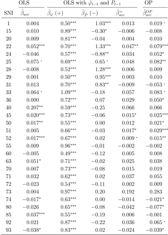
In Table 5 we can get a view of the bias of OLS compared to OLS with included controls for endogeneous input and exit choice, and with OP estimation.
OLS OLS with ^'t 1 and ^Pt 1 OP
SNI ^acc ^'^ (+) ^P^ ( ) ^acc+ ^accOP
1 0:004 0:50 1:03 0:013 0:019 15 0:010 0:89 0:30 0:006 0:008 20 0:009 0:81 0:04 0:004 0:010 22 0:052 0:70 1:33 0:047 0:079 24 0:046 0:57 0:88 0:034 0:052 25 0:075 0:69 0:65 0:048 0:082 28 0:008 0:52 1:28 0:006 0:009 29 0:001 0:50 0:95 0:003 0:010 31 0:013 0:70 0:83 0:009 0:053 33 0:064 1:09 0:18 0:057 0:083 36 0:000 0:72 0:07 0:029 0:050 40 0:207 0:59 0:25 0:066 0:066 45 0:020 0:73 0:06 0:015 0:025 50 0:017 0:55 0:00 0:012 0:021 51 0:005 0:66 0:03 0:017 0:029 52 0:017 0:67 0:02 0:009 0:015 55 0:009 0:96 0:01 0:002 0:002 60 0:005 0:49 0:12 0:005 0:008 63 0:051 0:71 0:02 0:025 0:038 70 0:007 0:73 0:08 0:015 0:019 71 0:032 0:62 0:02 0:037 0:055 72 0:023 0:54 0:11 0:002 0:009 73 0:004 0:97 0:20 0:192 0:283 74 0:017 0:63 0:00 0:014 0:021 80 0:026 0:65 0:08 0:042 0:077 85 0:037 0:55 0:19 0:006 0:001 92 0:021 0:87 0:22 0:036 0:065 93 0:038 0:83 0:02 0:024 0:039
Table 5: Bias of OLS production function estimates of the accessibility parameter ^
lacc in relation to OLS with the inclusion of lagged productivity ( ^') and lagged
survival probability ( ^P). The di¤erence between the …fth and second column constitutes the OLS bias. The value and sign of the ^'t 1 P^t 1, together with the
correlation between these variables and the accessibility, determine the size and direction of the bias. A positive '^ in general has a positive in‡uence on ^lacc
4.2.1 Tests
I perform three speci…cation tests: one focusing on the …rst estimation step in (3), and two on the last step in (6). The …rst one, suggested in Ackerberg et al. (2007), tests the validity of the assumption that the variable inputs (ln mt, ln lt)
are in fact variable, in the sense that they are decided after the realization of !t,
and thus uncorrelated with the idiosyncratic error t:This is done by comparing
the regression
ln yt= mln mt+ lln lt+ '0t(N etInvV olt; ln kbt; ln kmt; aget; ln acct) + 0t
with
ln yt= '1t(ln mt; ln lt; N etInvV olt; ln kbt; ln kmt; aget; ln acct) + 1t;
where ln mt and ln lt are included with higher order terms and interactions in
the proxy function '1
t. The resulting error terms 0t and 1t are then compared
using ANOVA. If they are not signi…cantly di¤erent from each other, then the intermediate inputs and labour are in fact chosen independently of 0
t; given '0t
as a proxy for individual heterogeneity and productivity (in period t). If they do di¤er, then there is residual correlation between these inputs and the error term in the …rst equation, and there is either a dynamic e¤ect of earlier choices of these inputs, or these inputs are not entirely variable conditional on '0
t (not adjusting
to current levels of predetermined inputs)16. And in fact, this test rejects the null
of equality in all industries, both when only labour is included in '1t and when
both inputs are included, which suggests that both of these inputs are either not variable, or they are dynamic.
The second and third tests are due to Olley and Pakes and test the validity of their approach by including lagged inputs in the third-stage estimating equation. First they include the presumed variable inputs, labour and intermediate inputs:
ln yt bmln mt blln lt= kbln kbt+ kmln kmt+ ageaget+ accln acct+
+ g Pbt 1;'bt 1 kbln kbt 1 kmln kmt 1 ageaget 1 accln acct 1 +
+ mln mt 1+ lln lt 1+ t+ t (7)
and second, they include the predetermined capital inputs and productivity shifter age. Here I also include accessibility as a predetermined productivity shifter:
16Another possibility is of course that '0
t is wrongly speci…ed and does not represent !t
su¢ ciently close. Note the di¤erence between dynamic and variable: dynamic means that the inputs are dependent on earlier choices (error terms in previous periods), while variable means that they are adjusted in response to performance !t.
ln yt bmln mt blln lt= kbln kbt+ kmln kmt+ ageaget+ accln acct+
+ g Pbt 1;'bt 1 kbln kbt 1 kmln kmt 1 ageaget 1 accln acct 1 +
+ kbln kbt 1+ kmln kmt 1+ ageaget 1+ accln acct 1+ t+ t: (8)
If the inputs ln mt and labour ln lt are in fact variable, and if bm and bl are
correctly estimated in the …rst stage, then the left hand side of the …rst test (7) should be uncorrelated with the lagged values of intermediates and labour, ln mt 1
and ln lt 1. The same should hold if they are static, i.e. they only a¤ect current
output (in period t), and not output in later periods. Thus if this test fails, at least one of these two assumptions is wrong.
In the case of the second test (8), if the g function correctly transmits the e¤ects of the past productivity !t 1through the inverted investment control proxy
function in (5) and the current productivity threshold !t, then there should be little
variation left for past levels of the state variables (capital, age and accessibility). However, the power of these tests have been questioned (Ackerberg, Caves, and Frazer, 2006). Especially in the latter test, the risk of multicollinearity between both the past and current levels of the state variables, and between the past levels inside and outside the non-parametric function g, is high. Accessibility, as well as the two types of capital, are inherently persistent.
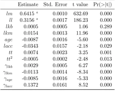
The test for lagged intermediate inputs (lm) and labour (ll) for the whole dataset is shown in Table 6. The parameters of the lagged variables are signi…cantly separate from zero, but their values are small compared to the parameters of the original speci…cation, which are also not greatly a¤ected.
The result of the second test, for lagged state variables, is found in Table 7, again for the whole dataset. Here the pattern is di¤erent. The parameters of the lagged state variables are highly signi…cant. In all cases, the sum of the past and current parameter is approximately equal to the original estimate, which is an ob-vious sign of the multicollinearity mentioned above. Of course, the state variables are as such very serially correlated, and this result might be expected. This result casts doubt on the relevance of this method for the estimation of accessibility elas-ticities. It is also possible that adjustments of production to changing accessibility takes longer than one year, which is the forward-looking time span used here.
Estimate Std. Error t value Pr(>jtj) lm 0.6415 a 0.0010 632.69 0.000 ll 0.3156 a 0.0017 186.23 0.000 lkb 0.0028 0.0003 9.21 0.000 lkm 0.0137 0.0010 14.16 0.000 age -0.0172 0.0003 -56.68 0.000 lacc 0.1045 0.0027 38.11 0.000 tt 0.0035 0.0022 1.57 0.117 tt2 -0.0002 0.0002 -0.72 0.472 lm -0.0042 0.0011 -3.93 0.000 ll -0.0191 0.0018 -10.63 0.000 aThe estimates for lm and ll are the same as in
Ta-ble 19 (…rst stage of estimation).
Table 6: Test for signi…cance of lagged values of ln m and ln l ( lm and ll).
De-pendent variable: ly bmln m blln l. All industries.
Estimate Std. Error t value Pr(>jtj) lm 0.6415a 0.0010 632.69 0.000 ll 0.3156a 0.0017 186.23 0.000 lkb 0.0005 0.0005 1.06 0.289 lkm 0.0154 0.0013 11.96 0.000 age -0.0087 0.0016 -5.60 0.000 lacc -0.0343 0.0157 -2.18 0.029 tt 0.0074 0.0023 3.25 0.001 tt2 -0.0005 0.0002 -2.48 0.013 lkb 0.0029 0.0005 6.27 0.000 lkm -0.0113 0.0014 -8.34 0.000 age -0.0085 0.0016 -5.33 0.000 lacc 0.1372 0.0161 8.52 0.000 aThe estimates for lm and ll are the same as in
Ta-ble 19 (…rst stage of estimation).
Table 7: Test for signi…cance of lagged values of lkb, lkm, age and lacc ( lkb etc.).
4.3
Robustness of estimates
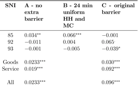
In order to assess the robustness of the production elasticities with respect to accessibility, three di¤erent travel impedance barriers over the Strait have been used, resulting in three di¤erent accessibility changes between the years before 2000 and the years after (see Table 2). The results are presented in Table 8. It shows that the level of the assumed barrier matters a lot for the estimates.
SNI A - no extra barrier B - 24 min uniform HH and MC C - original barrier 1 0:019 0:018: 0:019: 15 0:016 0:010 0:008 20 0:009 0:011 0:010 22 0:049 0:077 0:079 24 0:019 0:050 0:052 25 0:048: 0:082 0:082 28 0:004 0:009 0:009 29 0:003 0:007 0:010 31 0:039 0:058 0:053: 33 0:098 0:104 0:083: 36 0:034 0:034 0:050 40 0:107 0:078 0:066 45 0:041 0:058 0:025 50 0:032 0:037 0:021 51 0:028 0:043 0:029 52 0:031 0:039 0:015 55 0:020 0:020 0:002 60 0:024 0:042 0:008 63 0:088 0:082 0:038 70 0:029 0:036: 0:019 71 0:015 0:037 0:055 72 0:030 0:027 0:009 73 0:115 0:130 0:283 74 0:023 0:048 0:021 80 0:044: 0:049: 0:077
Robustness of accessibility estimates with regard to speci…cation of the barrier reduction of the …xed link. Boldface means signi…cant on the 5 % level. Continued on next page.
SNI A - no extra barrier B - 24 min uniform HH and MC C - original barrier 85 0:034 0:066 0:001 92 0:011 0:004 0:065: 93 0:001 0:005 0:039 Goods 0:0233 0:030 Service 0:019 0:092 All 0:0233 0:096
Table 8: Accessibility estimates with di¤erent speci…cations of the barrier after the introduction of the …xed link: cases A, B and C (see Table 2). HH = Helsingborg– Helsingør, MC = Malmö–Copenhagen. Boldface means signi…cant on the 5 % level.
4.4
Evaluation in the time dimension
In order to assess the relationship between the performance measure and accessi-bility in the time dimension, the above OP regressions were repeated on all the data (pooled industries), but now without the accessibility variable. The residuals from this regression was used as a technical e¢ ciency performance measure, which was aggregated zonewise and di¤erenced with 5-year intervals17. These di¤erences
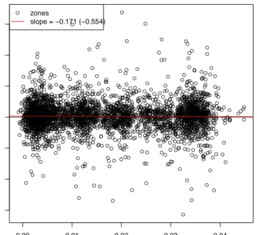
were then regressed against 5-year di¤erences of accessibility plus year dummies, and plotted together with the data, see
From this plot and the t-value of the slope coe¢ cient, we cannot reject hy-pothesis that there is no long-term e¤ect of higher accessibility on geographic productivity (hypothesis 3 above), at least not in a …ve year period. Admittedly, …ve years is not very long in the perspective of the life span of an infrastructure like this— therefore this results begs for continued studies on longer panel data sets.
17The aggregation of the residuals were weighted by the output share. Olley and Pakes (1996)
erroneously use the exponential of the residual as a productivity measure for post-analysis, which has a great impact because of the presence of extreme outliers. In this case, the productivity also has to be aggregated geometrically, not arithmetically.